
Hybrid Learning Moth Search Algorithm for Solving Multidimensional Knapsack Problems

Abstract
:1. Introduction
- A novel Baldwinian learning strategy based on Cauchy distribution is proposed, the analysis and experiment of which show this strategy is more effective than the Baldwin learning strategy based on Gaussian distribution.
- Combined with Baldwin learning, GHS is an effective global search operator to enhance the exploration ability of HLMS. Meanwhile, the pitch adjustment process based on dimensional learning can generate a large jump in the search process.
- To reduce computation costs, the proposed HLMS triggers Baldwin learning and GHS learning with a certain probability in each iteration.
- Exploration and exploitation are two common and fundamental features of any optimization method. In the evolution of HLMS, Lévy flight and GHS learning are mainly responsible for exploration, whilst flight straightly and Baldwinian mainly implement exploitation.
2. Preliminaries
2.1. Moth Search Algorithm
| Algorithm 1. Moth search algorithm |
| Begin Step 1: Initialization. Set the maximum iteration number MaxGen and iteration counter G = 1; Initialize the parameters max walk step Smax, the index , and acceleration factor . According to uniform distribution, the population with NP individuals is randomly initialized. Step 2: Fitness calculation. Compute the initial objective function values of each individual according to their position. Memory the best individual (denotes as Xbest). Step 3: While (G < MaxGen) do Divide the whole population into two subpopulations with equal size: subpopulation1 and subpopulation2, based on their fitness. Update subpopulation1 by using Lévy flight operator (Equation (4)). Update subpopulation2 by using flight straightly operator (Equation (7)). Evaluate the objective function values of each individual and update Xbest. G = G + 1. Sort the population by fitness. Step 4: End while Step 5: Output: the best results. End. |
2.2. Baldwin Effect and Baldwinian Learning
2.3. Global-Best HS Algorithm
| Algorithm 2. The Global-best HS algorithm (GHS) |
| Begin For each do /*n is the dimension of the problem*/ If U(0, 1) ≤ HMCR then /* memory consideration*/ , where If U(0,1) ≤ PAR (t) then /*pitch adjustment*/ , where best is the best harmony in the HM and Else /*random selection*/ End. |
3. The Proposed HLMS for the MKP
3.1. Population Initialization
3.2. Solution Representation
3.3. Quick Repair Operator
| Algorithm 3. The quick repair operator base on the scaled pseudo-utility |
| Begin Step 1: Input. . Step 2: Calculation. Calculate the current total consumption of each resource. . Step 3: Repair process. For j = n to 1 do If then Break. else if = 1 then Set = 0, and End End Step 4: Optimization process. For j = 1 to n do If and then Set and End End Step 5: Output: . End. |
3.4. Procedure of HLMS for MKP
| Algorithm 4. Procedure of HLMS for MKP |
Begin
3.2 Update subpopulation1 by Lévy flight operator. 3.3 Update subpopulation2 by flight straightly operator. 3.4 GHS search If U(0, 1) ≤ 0.5 Apply GHS algorithm on each individual X and generate the trial individual Y. Choose the best one of X and Y to enter the next generation. 3.5 Baldwinian Learning If U(0, 1) ≤ 0.5 Apply Baldwinin learning strategy on each individual X and generate the trial individual Y. Choose the best one of X and Y to enter the next generation. 3.6 Apply transform function to obtain the potential solution of MKP. 3.7 Repair the potential solution by Algorithm 3. 3.8 Evaluate the fitness of the population and record the global best fitness. G = G + 1. 3.9 Sort the population by fitness. Step 4: End while Step 5: Output: the best results. End. |
3.5. Computational Complexity of One Iteration of HLMS
- (1)
- The initialization of HLMS requires O(NP × n) time, where NP denotes the population size, and n is the dimension of MKP (the number of the items).
- (2)
- The discretization process of NP moth individual costs O(NP × n) time.
- (3)
- The quick repair operator takes O(n × m) time, where m is the constraints of the MKP instance.
- (4)
- Fitness evaluation has O(NP) time.
- (5)
- Lévy flight operator has O(NP1 × n) time, where NP1 is the number of individuals of subpopulation1.
- (6)
- Flight straightly operator has O(NP2 × n) time, where NP2 is the number of individuals of subpopulation2.
- (7)
- GHS learning requires O(NP × n) time.
- (8)
- Baldwinian learning requires O(NP × n) time.
- (9)
- Sort the population based on Quick sort algorithm and it takes time O(NPlogNP).
4. Experimental Studies
4.1. Benchmark Test Functions
4.2. Experimental Environment and Parameters Setting
- Modified binary particle swarm optimization (MBPSO) [78];
- Chaotic binary particle swarm optimization with time-varying acceleration coefficients (CBPSOTVAC) [79];
- Binary PSO with time-varying acceleration coefficients (BPSOTVAC) [79];
- Modified multi-verse optimization (MMVO) algorithm [17];
- New binary particle swarm optimization with immunity-clonal algorithm (NPSOCLA) [80];
- Binary gravitational search algorithm (BGSA) [81];
- Binary hybrid topology particle swarm optimization (BHTPSO) [81];
- Binary hybrid topology particle swarm optimization quadratic interpolation (BHTPSO-QI) [81];
- New binary particle swarm optimization (NBPSO) [81];
- Binary version of PSO (BPSO) [82];
- Binary version of the salp swarm algorithm (BSSA) [84];
- Binary version of the modified whale optimization algorithm (BIWOA) [85];
- Binary version of the sin-cosine algorithm (BSCA) [86].
- Best value (Best):
- Worst value (Worst):
- Mean value (Mean):
- Standard deviation (Std):
- Success rate (SR):
- Percent deviation (PDev):
- Average error (AE):
- Percentage gap (Gap):
4.3. Comparisons on the Small-Scale Test Set
4.4. Comparisons on the Medium-Scale Test Set
4.5. Comparisons on the Large-Scale Test Set
4.5.1. Performance Comparison on Test Set III (cb1–cb3)
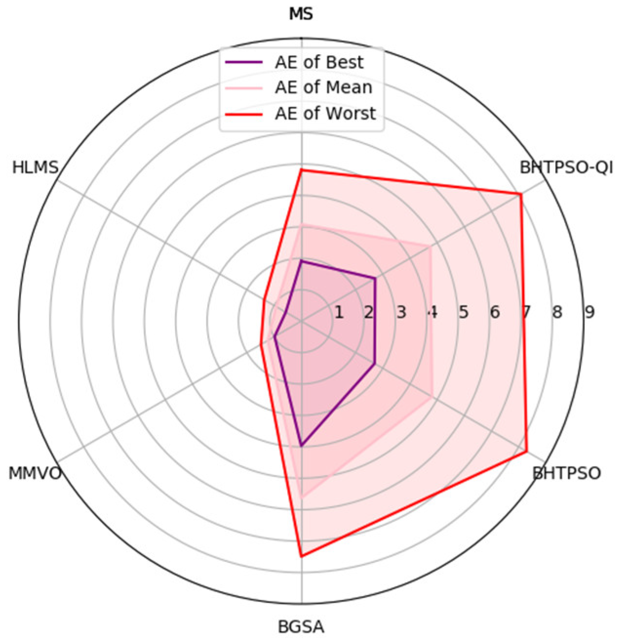
4.5.2. Performance Comparison on Test Set III (cb4–cb6)
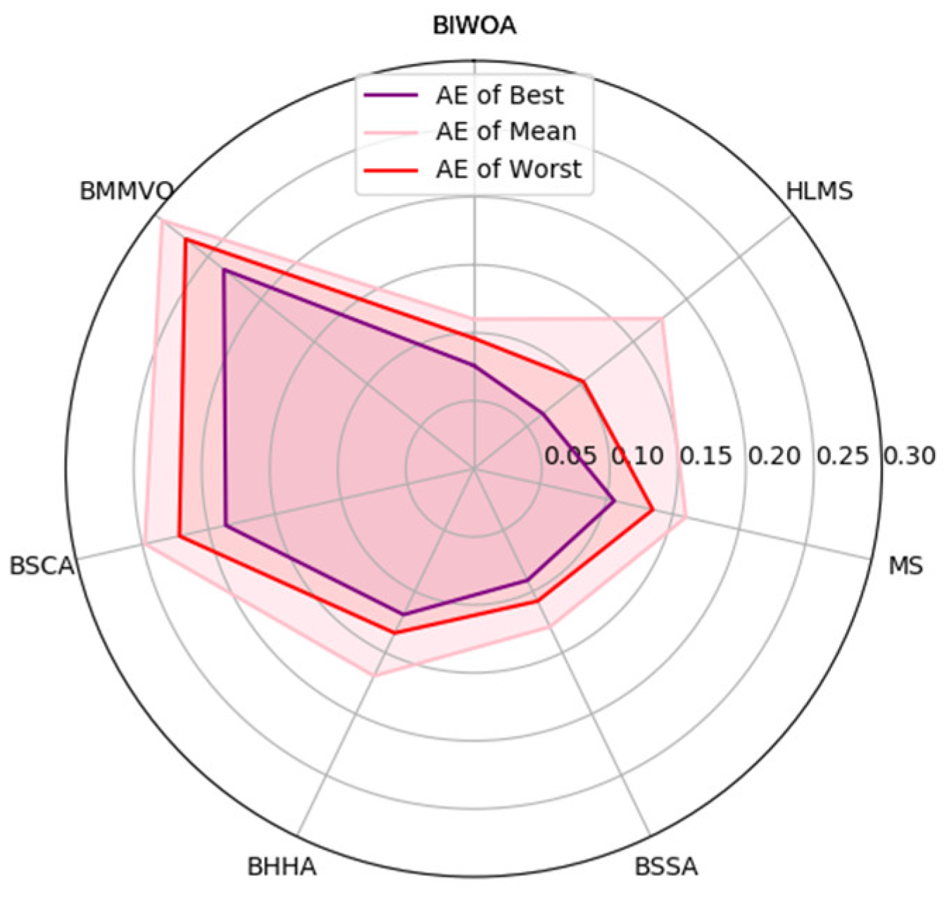
4.5.3. Performance Comparison on Test Set IV
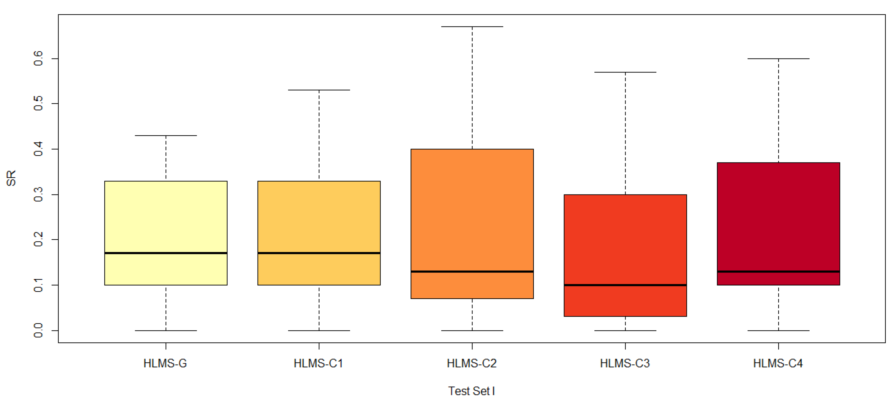
4.6. Sensitivity Analysis on the Positional Parameter and the Scale Parameter
4.7. The Effectiveness of the Two Components in HLMS
4.8. Discussion
5. Conclusions and Future Work
Author Contributions
Funding
Institutional Review Board Statement
Informed Consent Statement
Data Availability Statement
Conflicts of Interest
References
- Toyoda, Y. A simplified algorithm for obtaining approximate solutions to zero-one programming problems. Manag. Sci. 1975, 21, 1417–1427. [Google Scholar] [CrossRef]
- Vasquez, M.; Vimont, Y. Improved results on the 0–1 multidimensional knapsack problem. Eur. J. Oper. Res. 2005, 165, 70–81. [Google Scholar] [CrossRef]
- Feng, Y.; Yang, J.; Wu, C.; Lu, M.; Zhao, X.-J. Solving 0-1 knapsack problems by chaotic monarch butterfly optimization algorithm with Gaussian mutation. Memetic Comput. 2018, 10, 135–150. [Google Scholar] [CrossRef]
- Weingartner, H.M.; Ness, D.N. Methods for the solution of the multidimensional 0/1 knapsack problem. Oper. Res. 1967, 15, 83–103. [Google Scholar] [CrossRef]
- Drake, J.H.; Özcan, E.; Burke, E.K. A case study of controlling crossover in a selection hyper-heuristic framework using the multidimensional knapsack problem. Evol. Comput. 2016, 24, 113–141. [Google Scholar] [CrossRef] [Green Version]
- Gilmore, P.; Gomory, R.E. The theory and computation of knapsack functions. Oper. Res. 1966, 14, 1045–1074. [Google Scholar] [CrossRef]
- Shih, W. A branch and bound method for the multiconstraint zero-one knapsack problem. J. Oper. Res. Soc. 1979, 30, 369–378. [Google Scholar] [CrossRef]
- Boussier, S.; Vasquez, M.; Vimont, Y.; Hanafi, S.; Michelon, P. A multi-level search strategy for the 0-1 Multidimensional Knapsack Problem. Discret. Appl. Math. 2010, 158, 97–109. [Google Scholar] [CrossRef]
- Lai, X.; Hao, J.-K.; Glover, F.; Lü, Z. A two-phase tabu-evolutionary algorithm for the 0-1 multidimensional knapsack problem. Inf. Sci. 2018, 436, 282–301. [Google Scholar] [CrossRef]
- Chih, M. Three pseudo-utility ratio-inspired particle swarm optimization with local search for multidimensional knapsack problem. Swarm Evol. Comput. 2018, 39, 279–296. [Google Scholar] [CrossRef]
- Haddar, B.; Khemakhem, M.; Hanafi, S.; Wilbaut, C. A hybrid quantum particle swarm optimization for the multidimensional knapsack problem. Eng. Appl. Artif. Intell. 2016, 55, 1–13. [Google Scholar] [CrossRef]
- Lai, X.; Hao, J.-K.; Fu, Z.-H.; Yue, D. Diversity-preserving quantum particle swarm optimization for the multidimensional knapsack problem. Expert Syst. Appl. 2020, 149, 113310. [Google Scholar] [CrossRef]
- Wang, L.; Wang, S.-y.; Xu, Y. An effective hybrid EDA-based algorithm for solving multidimensional knapsack problem. Expert Syst. Appl. 2012, 39, 5593–5599. [Google Scholar] [CrossRef]
- Li, Z.; Tang, L.; Liu, J. A memetic algorithm based on probability learning for solving the multidimensional knapsack problem. IEEE Trans. Cybern. 2020, 54, 2284–2299. [Google Scholar] [CrossRef] [PubMed]
- Luo, K.; Zhao, Q. A binary grey wolf optimizer for the multidimensional knapsack problem. Appl. Soft Comput. 2019, 83, 105645. [Google Scholar] [CrossRef]
- Zhang, B.; Pan, Q.K.; Zhang, X.L.; Duan, P.Y. An effective hybrid harmony search-based algorithm for solving multidimensional knapsack problems. Appl. Soft Comput. 2015, 29, 288–297. [Google Scholar] [CrossRef]
- Abdel-Basset, M.; El-Shahat, D.; Faris, H.; Mirjalili, S. A binary multi-verse optimizer for 0-1 multidimensional knapsack problems with application in interactive multimedia systems. Comput. Ind. Eng. 2019, 132, 187–206. [Google Scholar] [CrossRef]
- García, J.; Maureira, C. A KNN quantum cuckoo search algorithm applied to the multidimensional knapsack problem. Appl. Soft Comput. 2021, 102, 107077. [Google Scholar] [CrossRef]
- Bolaji, A.L.a.; Okwonu, F.Z.; Shola, P.B.; Balogun, B.S.; Adubisi, O.D. A modified binary pigeon-inspired algorithm for solving the multi-dimensional knapsack problem. J. Intell. Syst. 2021, 30, 90–103. [Google Scholar] [CrossRef]
- Feng, Y.; Wang, G.-G. A binary moth search algorithm based on self-learning for multidimensional knapsack problems. Future Gener. Comput. Syst. 2022, 126, 48–64. [Google Scholar] [CrossRef]
- Gupta, S.; Su, R.; Singh, S. Diversified sine-cosine algorithm based on differential evolution for multidimensional knapsack problem. Appl. Soft Comput. 2022, 130, 109682. [Google Scholar] [CrossRef]
- Abdel-Basset, M.; Mohamed, R.; Sallam, K.M.; Chakrabortty, R.K.; Ryan, M.J. BSMA: A novel metaheuristic algorithm for Multi-dimensional knapsack problems: Method and comprehensive analysis. Comput. Ind. Eng. 2021, 159, 107469. [Google Scholar] [CrossRef]
- Li, W.; Yao, X.; Zhang, T.; Wang, R.; Wang, L. Hierarchy ranking method for multimodal multi-objective optimization with local pareto fronts. IEEE Trans. Evol. Comput. 2022, 27, 98–110. [Google Scholar] [CrossRef]
- Cacchiani, V.; Iori, M.; Locatelli, A.; Martello, S. Knapsack problems-An overview of recent advances. Part II: Multiple, multidimensional, and quadratic knapsack problems. Comput. Oper. Res. 2022, 143, 105693. [Google Scholar] [CrossRef]
- Gao, D.; Wang, G.-G.; Pedrycz, W. Solving fuzzy job-shop scheduling problem using DE algorithm improved by a selection mechanism. IEEE Trans. Fuzzy Syst. 2020, 28, 3265–3275. [Google Scholar] [CrossRef]
- Wang, G.-G.; Gao, D.; Pedrycz, W. Solving multi-objective fuzzy job-shop scheduling problem by a hybrid adaptive differential evolution algorithm. IEEE Trans. Ind. Inform. 2022, 18, 8519–8528. [Google Scholar] [CrossRef]
- Shadkam, E.; Bijari, M. A novel improved cuckoo optimisation algorithm for engineering optimisation. Int. J. Artif. Intell. Soft Comput. 2020, 7, 164–177. [Google Scholar] [CrossRef]
- Parashar, S.; Senthilnath, J.; Yang, X.-S. A novel bat algorithm fuzzy classifier approach for classification problems. Int. J. Artif. Intell. Soft Comput. 2017, 6, 108–128. [Google Scholar] [CrossRef]
- Wang, G.-G.; Deb, S.; Gandomi, A.H.; Alavi, A.H. Opposition-based krill herd algorithm with cauchy mutation and position clamping. Neurocomputing 2016, 177, 147–157. [Google Scholar] [CrossRef]
- Wang, G.-G.; Guo, L.; Gandomi, A.H.; Hao, G.S.; Wang, H. Chaotic krill herd algorithm. Inf. Sci. 2014, 274, 17–34. [Google Scholar] [CrossRef]
- Li, W.; Wang, G.-G.; Alavi, A.H. Learning-based elephant herding optimization algorithm for solving numerical optimization problems. Knowl.-Based Syst. 2020, 195, 105675. [Google Scholar] [CrossRef]
- Wang, G.-G.; Deb, S.; Cui, Z. Monarch butterfly optimization. Neural Comput. Appl. 2019, 31, 1995–2014. [Google Scholar] [CrossRef] [Green Version]
- Feng, Y.; Deb, S.; Wang, G.-G.; Alavi, A.H. Monarch butterfly optimization: A comprehensive review. Expert Syst. Appl. 2021, 168, 114418. [Google Scholar] [CrossRef]
- Ma, L.; Cheng, S.; Shi, Y. Enhancing learning efficiency of brain storm optimization via orthogonal learning design. IEEE Trans. Syst. Man Cybern. Syst. 2020, 51, 6723–6742. [Google Scholar] [CrossRef]
- Yu, H.; Li, W.; Chen, C.; Liang, J.; Gui, W.; Wang, M.; Chen, H. Dynamic Gaussian bare-bones fruit fly optimizers with abandonment mechanism: Method and analysis. Eng. Comput. 2020, 38, 743–771. [Google Scholar] [CrossRef]
- Mirjalili, S.; Lewis, A. The whale optimization algorithm. Adv. Eng. Softw. 2016, 95, 51–67. [Google Scholar] [CrossRef]
- Zhou, Y.; Bao, Z.; Luo, Q.; Zhang, S. A complex-valued encoding wind driven optimization for the 0-1 knapsack problem. Appl. Intell. 2017, 46, 684–702. [Google Scholar] [CrossRef]
- Song, J.; Chen, C.; Heidari, A.A.; Liu, J.; Yu, H.; Chen, H. Performance optimization of annealing salp swarm algorithm: Frameworks and applications for engineering design. J. Comput. Des. Eng. 2022, 9, 633–669. [Google Scholar] [CrossRef]
- Gezici, H.; Livatyalı, H. Chaotic Harris hawks optimization algorithm. J. Comput. Des. Eng. 2022, 9, 216–245. [Google Scholar] [CrossRef]
- Chou, J.S.; Truong, D.N. A novel metaheuristic optimizer inspired by behavior of jellyfish in ocean. Appl. Math. Comput. 2021, 389, 125535. [Google Scholar] [CrossRef]
- Wang, L.Y.; Cao, Q.J.; Zhang, Z.X.; Mirjalili, S.; Zhao, W.G. Artificial rabbits optimization: A new bio-inspired meta-heuristic algorithm for solving engineering optimization problems. Eng. Appl. Artif. Intell. 2022, 114, 31. [Google Scholar] [CrossRef]
- Abdollahzadeh, B.; Gharehchopogh, F.S.; Khodadadi, N.; Mirjalili, S. Mountain Gazelle Optimizer: A new Nature-inspired Metaheuristic Algorithm for Global Optimization Problems. Adv. Eng. Softw. 2022, 174, 34. [Google Scholar] [CrossRef]
- Chen, C.; Wang, X.; Yu, H.; Wang, M.; Chen, H. Dealing with multi-modality using synthesis of Moth-flame optimizer with sine cosine mechanisms. Math. Comput. Simul. 2021, 188, 291–318. [Google Scholar] [CrossRef]
- Wang, G.-G. Moth search algorithm: A bio-inspired metaheuristic algorithm for global optimization problems. Memetic Comput. 2018, 10, 151–164. [Google Scholar] [CrossRef]
- Li, J.; Yang, Y.H.; An, Q.; Lei, H.; Deng, Q.; Wang, G.G. Moth Search: Variants, Hybrids, and Applications. Mathematics 2022, 10, 4162. [Google Scholar] [CrossRef]
- Elaziz, M.A.; Xiong, S.; Jayasena, K.; Li, L. Task scheduling in cloud computing based on hybrid moth search algorithm and differential evolution. Knowl.-Based Syst. 2019, 169, 39–52. [Google Scholar] [CrossRef]
- Strumberger, I.; Sarac, M.; Markovic, D.; Bacanin, N. Moth search algorithm for drone placement problem. Int. J. Comput. 2018, 3, 75–80. [Google Scholar]
- Strumberger, I.; Tuba, E.; Bacanin, N.; Beko, M.; Tuba, M. Hybridized moth search algorithm for constrained optimization problems. In Proceedings of the 2018 International Young Engineers Forum (YEF-ECE), Monte de Caparica, Portugal, 4 May 2018; pp. 1–5. [Google Scholar]
- Feng, Y.; Wang, G.-G. Binary moth search algorithm for discounted {0-1} knapsack problem. IEEE Access 2018, 6, 10708–10719. [Google Scholar] [CrossRef]
- Feng, Y.; An, H.; Gao, X. The importance of transfer function in solving set-union knapsack problem based on discrete moth search algorithm. Mathematics 2019, 7, 17. [Google Scholar] [CrossRef] [Green Version]
- Feng, Y.; Yi, J.-H.; Wang, G.-G. Enhanced moth search algorithm for the set-union knapsack problems. IEEE Access 2019, 7, 173774–173785. [Google Scholar] [CrossRef]
- Cui, Z.; Xue, F.; Cai, X.; Cao, Y.; Wang, G.-G.; Chen, J. Detection of malicious code variants based on deep learning. IEEE Trans. Ind. Inform. 2018, 14, 3187–3196. [Google Scholar] [CrossRef]
- Zhang, J.; Pan, L.; Han, Q.-L.; Chen, C.; Wen, S.; Xiang, Y. Deep Learning Based Attack Detection for Cyber-Physical System Cybersecurity: A Survey. IEEE/CAA J. Autom. Sin. 2021, 9, 377–391. [Google Scholar] [CrossRef]
- Wang, F.; Wang, X.; Sun, S. A reinforcement learning level-based particle swarm optimization algorithm for large-scale optimization. Inf. Sci. 2022, 602, 298–312. [Google Scholar] [CrossRef]
- Wang, L.; Pan, Z.; Wang, J. A review of reinforcement learning based intelligent optimization for manufacturing scheduling. Complex Syst. Model. Simul. 2021, 1, 257–270. [Google Scholar] [CrossRef]
- Zhou, T.; Chen, M.; Zou, J. Reinforcement learning based data fusion method for multi-sensors. IEEE/CAA J. Autom. Sin. 2020, 7, 1489–1497. [Google Scholar] [CrossRef]
- Zheng, R.-z.; Zhang, Y.; Yang, K. A transfer learning-based particle swarm optimization algorithm for travelling salesman problem. J. Comput. Des. Eng. 2022, 9, 933–948. [Google Scholar] [CrossRef]
- Bingjie, X.; Deming, L. Q-Learning-based teaching-learning optimization for distributed two-stage hybrid flow shop scheduling with fuzzy processing time. Complex Syst. Model. Simul. 2022, 2, 113–129. [Google Scholar] [CrossRef]
- Wang, G.-G.; Tan, Y. Improving metaheuristic algorithms with information feedback models. IEEE Trans. Cybern. 2019, 49, 542–555. [Google Scholar] [CrossRef]
- Chen, C.; Wang, X.; Yu, H.; Zhao, N.; Wang, M.; Chen, H.; Kumarappan, N. An Enhanced Comprehensive Learning Particle Swarm Optimizer with the Elite-Based Dominance Scheme. Complexity 2020, 2020, 1–24. [Google Scholar] [CrossRef]
- Gong, M.; Jiao, L.; Zhang, L. Baldwinian learning in clonal selection algorithm for optimization. Inf. Sci. 2010, 180, 1218–1236. [Google Scholar] [CrossRef]
- Hinton, G.E.; Nowlan, S.J. How learning can guide evolution. In Adaptive Individuals in Evolving Populations: Models and Algorithms; Addison-Wesley Longman Publishing Co., Inc.: Boston, MA, USA, 1996; Volume 26, pp. 447–454. [Google Scholar]
- Qi, Y.; Liu, F.; Liu, M.; Gong, M.; Jiao, L. Multi-objective immune algorithm with Baldwinian learning. Appl. Soft Comput. 2012, 12, 2654–2674. [Google Scholar] [CrossRef]
- Zhang, C.; Chen, J.; Xin, B. Distributed memetic differential evolution with the synergy of Lamarckian and Baldwinian learning. Appl. Soft Comput. 2013, 13, 2947–2959. [Google Scholar] [CrossRef]
- Geem, Z.W.; Kim, J.H.; Loganathan, G.V. A new heuristic optimization algorithm: Harmony search. Simulation 2001, 76, 60–68. [Google Scholar] [CrossRef]
- Omran, M.G.H.; Mahdavi, M. Global-best harmony search. Appl. Math. Comput. 2008, 198, 643–656. [Google Scholar] [CrossRef]
- Xiang, W.L.; An, M.Q.; Li, Y.Z.; He, R.C.; Zhang, J.F. A novel discrete global-best harmony search algorithm for solving 0-1 knapsack problems. Discret. Dyn. Nat. Soc. 2014, 2014, 1–12. [Google Scholar] [CrossRef] [Green Version]
- Keshtegar, B.; Sadeq, M.O. Gaussian global-best harmony search algorithm for optimization problems. Soft Comput. 2017, 21, 7337–7349. [Google Scholar] [CrossRef]
- El-Abd, M. An improved global-best harmony search algorithm. Appl. Math. Comput. 2013, 222, 94–106. [Google Scholar] [CrossRef]
- Peng, Y.; Lu, B.-L. Hybrid learning clonal selection algorithm. Inf. Sci. 2015, 296, 128–146. [Google Scholar] [CrossRef]
- Lan, K.-T.; Lan, C.-H. Notes on the distinction of Gaussian and Cauchy mutations. In Proceedings of the 2008 Eighth International Conference on Intelligent Systems Design and Applications, Kaohsuing, Taiwan, 26–28 November 2008; pp. 272–277. [Google Scholar]
- Mahdavi, M.; Fesanghary, M.; Damangir, E. An improved harmony search algorithm for solving optimization problems. Appl. Math. Comput. 2007, 188, 1567–1579. [Google Scholar] [CrossRef]
- Xiao, S.; Wang, W.; Wang, H.; Tan, D.; Wang, Y.; Yu, X.; Wu, R. An Improved Artificial Bee Colony Algorithm Based on Elite Strategy and Dimension Learning. Mathematics 2019, 7, 289. [Google Scholar] [CrossRef] [Green Version]
- Chu, P.C.; Beasley, J.E. A genetic algorithm for the multidimensional knapsack problem. J. Heuristics 1998, 4, 63–86. [Google Scholar] [CrossRef]
- Puchinger, J.; Raidl, G.R.; Pferschy, U. The multidimensional knapsack problem: Structure and algorithms. Inf. J. Comput. 2010, 22, 250–265. [Google Scholar] [CrossRef] [Green Version]
- Senju, S.; Toyoda, Y. An approach to linear programming with 0-1 variables. Manag. Sci. 1968, 15, B196–B207. [Google Scholar] [CrossRef]
- Freville, A. Hard 0-1 multiknapsack test problems for size reduction methods. Investig. Oper. 1990, 1, 251–270. [Google Scholar]
- Bansal, J.C.; Deep, K. A modified binary particle swarm optimization for knapsack problems. Appl. Math. Comput. 2012, 218, 11042–11061. [Google Scholar] [CrossRef]
- Chih, M.; Lin, C.-J.; Chern, M.-S.; Ou, T.-Y. Particle swarm optimization with time-varying acceleration coefficients for the multidimensional knapsack problem. Appl. Math. Model. 2014, 38, 1338–1350. [Google Scholar] [CrossRef]
- Dina, E.-G.; Badr, A.; Abd El Azeim, M. New binary particle swarm optimization with immunity-clonal algorithm. J. Comput. Sci. 2013, 9, 1534. [Google Scholar]
- Beheshti, Z.; Shamsuddin, S.M.; Hasan, S. Memetic binary particle swarm optimization for discrete optimization problems. Inf. Sci. 2015, 299, 58–84. [Google Scholar] [CrossRef]
- Kennedy, J.; Eberhart, R.C. A discrete binary version of the particle swarm algorithm. In Proceedings of the 1997 IEEE International Conference on Systems, Man, and Cybernetics, Orlando, FL, USA, 12–15 October 1997; pp. 4104–4108. [Google Scholar]
- Aaha, B.; Sm, C.; Hf, D.; Ia, D.; Mm, E.; Hc, F. Harris hawks optimization: Algorithm and applications. Future Gener. Comput. Syst. 2019, 97, 849–872. [Google Scholar]
- Mirjalili, S.; Gandomi, A.H.; Mirjalili, S.Z.; Saremi, S.; Faris, H.; Mirjalili, S.M. Salp swarm algorithm: A bio-inspired optimizer for engineering design problems. Adv. Eng. Softw. 2017, 114, 163–191. [Google Scholar] [CrossRef]
- Abdel-Basset, M.; El-Shahat, D.; Sangaiah, A.K. A modified nature inspired meta-heuristic whale optimization algorithm for solving 0-1 knapsack problem. Int. J. Mach. Learn. Cybern. 2017, 10, 1–20. [Google Scholar] [CrossRef]
- Pinto, H.; Pea, A.; Valenzuela, M.; Fernández, A. A binary sine-cosine algorithm applied to the knapsack problem. In Proceedings of the Computer Science Online Conference, Zlin, Czech Republic, 24–27 April 2019; pp. 128–138. [Google Scholar]


| Parameters | Section | Description | Values |
|---|---|---|---|
| Smax | 2.1 | The max step used in Equation (5) | 1.0 |
| 2.1 | The acceleration factor used in Equation (7) | 0.618 | |
| 2.1 | The scale factor used in Equation (7) | a random number of uniform distribution in [0, 1] | |
| 2.1 | Parameter used in Equation (6) | 1.5 | |
| c | 2.2 | The strength of Baldwinian learning | A random number based on Cauchy distribution |
| PARmax | 2.3 | Parameter used in Equation (9) | 0.99 |
| PARmin | 2.3 | Parameter used in Equation (9) | 0.01 |
| HMCR | 2.3 | Parameter used in Algorithm 2 | 0.9 |
| NP | 3.4 | The population size | 50 |
| NFE | 3.4 | The maximal number of function evaluation | 100,000 |
| Prob. | n × m | Opt. | MS | HLMS | MBPSO | CBPSOTVAC | ||||
|---|---|---|---|---|---|---|---|---|---|---|
| SR | Std | SR | Std | SR | Std | SR | Std | |||
| Sento1 | 60 × 30 | 7772 | 0.17 | 54.46 | 0.90 | 33.73 | 0.16 | 43.23 | 0.39 | 357.78 |
| Sento2 | 60 × 30 | 8722 | 0.00 | 27.79 | 0.47 | 4.72 | 0.03 | 18.80 | 0.20 | 101.03 |
| HP1 | 28 × 4 | 3418 | 0.13 | 23.11 | 0.40 | 19.96 | 0.10 | 25.52 | 0.38 | 10.69 |
| HP2 | 35 × 4 | 3186 | 0.00 | 26.47 | 0.40 | 32.70 | 0.11 | 39.15 | 0.59 | 21.35 |
| PB1 | 27 × 4 | 3090 | 0.03 | 30.89 | 0.43 | 17.16 | 0.11 | 24.32 | 0.40 | 10.52 |
| PB2 | 34 × 4 | 3186 | 0.00 | 19.95 | 0.70 | 13.83 | 0.16 | 39.31 | 0.51 | 18.73 |
| PB4 | 29 × 2 | 95,168 | 0.00 | 894.68 | 0.30 | 1521.73 | 0.27 | 1803 | 0.84 | 875.1 |
| PB5 | 20 × 10 | 2139 | 0.17 | 23.88 | 0.70 | 21.26 | 0.08 | 24.36 | 0.80 | 6.83 |
| PB6 | 40 × 30 | 776 | 0.43 | 24.27 | 0.80 | 17.28 | 0.28 | 29.12 | 0.54 | 40.17 |
| PB7 | 37 × 30 | 1035 | 0.03 | 3.86 | 0.50 | 5.83 | 0.05 | 16.29 | 0.40 | 24.25 |
| Weing1 | 28 × 2 | 14,1278 | 0.90 | 214.94 | 0.93 | 89.77 | 0.82 | 250.43 | 0.92 | 281.98 |
| Weing2 | 28 × 2 | 130,883 | 0.30 | 5731.34 | 0.97 | 29.21 | 0.65 | 314.08 | 0.88 | 545.50 |
| Weing3 | 28 × 2 | 95,677 | 0.13 | 3767.42 | 0.80 | 1996.82 | 0.11 | 876.78 | 0.75 | 672.42 |
| Weing4 | 28 × 2 | 119,337 | 0.73 | 1329.64 | 0.37 | 711.43 | 0.76 | 1270.80 | 0.97 | 378.58 |
| Weing5 | 28 × 2 | 98,796 | 0.23 | 2671.33 | 1.00 | 0.00 | 0.52 | 1923.5 | 0.94 | 572.82 |
| Weing6 | 28 × 2 | 130,623 | 0.23 | 164.95 | 0.97 | 71.20 | 0.36 | 322.40 | 0.97 | 343.45 |
| Weing7 | 105 × 2 | 1,095,445 | 0.00 | 482.74 | 0.00 | 2872.29 | 0.02 | 1130.60 | 0.00 | 30,020.00 |
| Weing8 | 105 × 2 | 624,319 | 0.33 | 1966.37 | 0.03 | 1135.87 | 0.03 | 4704.30 | 0.20 | 75,169.00 |
| #Opt | 13 | 17 | 18 | 17 | ||||||
| #SR | 0 | 12 | 1 | 5 | ||||||
| #Std | 1 | 10 | 0 | 7 | ||||||
| MSR | 0.21 | 0.54 | 0.26 | 0.59 | ||||||
| Rank of MSR | 4 | 2 | 3 | 1 | ||||||
| p-value | 0.001 | 0.029 | 0.001 | 0.663 | 0.641 | 0.896 | ||||
| Prob. | n × m | Opt. | MS | HLMS | BIWOA | BMMVO | BSCA | BHHA | BSSA | |
|---|---|---|---|---|---|---|---|---|---|---|
| Weish01 | 30 × 5 | 4554 | Best | 4554 | 4554 | 4554 | 4554 | 4554 | 4554 | 4554 |
| Worst | 4477 | 4534 | 4554 | 4554 | 4534 | 4554 | 4554 | |||
| PDev | 0.38 | 0.18 | 0.00 | 0.00 | 0.09 | 0.00 | 0.00 | |||
| Weish02 | 30 × 5 | 4536 | Best | 4536 | 4536 | 4536 | 4536 | 4536 | 4536 | 4536 |
| Worst | 4440 | 4504 | 4536 | 4536 | 4536 | 4536 | 4536 | |||
| PDev | 0.38 | 0.02 | 0.00 | 0.00 | 0.00 | 0.00 | 0.00 | |||
| Weish03 | 30 × 5 | 4115 | Best | 4106 | 4115 | 4106 | 4106 | 4106 | 4106 | 4106 |
| Worst | 4106 | 4106 | 4106 | 4106 | 4106 | 4106 | 4106 | |||
| PDev | 0.22 | 0.19 | 3.97 | 3.05 | 0.00 | 2.24 | 3.97 | |||
| Weish04 | 30 × 5 | 4561 | Best | 4561 | 4561 | 4561 | 4561 | 4561 | 4561 | 4561 |
| Worst | 4505 | 4531 | 4561 | 4561 | 4561 | 4561 | 4561 | |||
| PDev | 0.37 | 0.09 | 0.00 | 0.00 | 0.00 | 0.00 | 0.00 | |||
| Weish05 | 30 × 5 | 4514 | Best | 4514 | 4514 | 4514 | 4514 | 4514 | 4514 | 4514 |
| Worst | 4514 | 4514 | 4514 | 4514 | 4514 | 4514 | 4514 | |||
| PDev | 0.00 | 0.00 | 0.00 | 0.00 | 0.00 | 0.00 | 0.00 | |||
| Weish06 | 40 × 5 | 5557 | Best | 5557 | 5557 | 5557 | 5557 | 5557 | 5557 | 5557 |
| Worst | 5502 | 5542 | 5542 | 5542 | 5542 | 5544 | 5557 | |||
| PDev | 0.40 | 0.09 | 0.12 | 0.14 | 0.14 | 0.02 | 0.00 | |||
| Weish07 | 40 × 5 | 5567 | Best | 5567 | 5567 | 5567 | 5567 | 5567 | 5567 | 5567 |
| Worst | 5360 | 5542 | 5567 | 5567 | 5567 | 5567 | 5567 | |||
| PDev | 0.53 | 0.03 | 0.00 | 0.00 | 0.00 | 0.00 | 0.00 | |||
| Weish08 | 40 × 5 | 5605 | Best | 5605 | 5605 | 5605 | 5605 | 5605 | 5605 | 5605 |
| Worst | 5478 | 5603 | 5605 | 5603 | 5603 | 5605 | 5605 | |||
| PDev | 0.30 | 0.01 | 0.00 | 0.03 | 0.01 | 0.00 | 0.00 | |||
| Weish09 | 40 × 5 | 5246 | Best | 5246 | 5246 | 5246 | 5246 | 5246 | 5246 | 5246 |
| Worst | 5185 | 5246 | 5246 | 5246 | 5246 | 5246 | 5246 | |||
| PDev | 0.08 | 0.00 | 0.00 | 0.00 | 0.00 | 0.00 | 0.00 | |||
| Weish10 | 50 × 5 | 6339 | Best | 6339 | 6339 | 6323 | 6303 | 6303 | 6303 | 6303 |
| Worst | 6255 | 6280 | 6303 | 6303 | 6303 | 6303 | 6303 | |||
| PDev | 0.55 | 0.04 | 0.31 | 0.56 | 0.56 | 0.56 | 0.56 | |||
| Weish11 | 50 × 5 | 5643 | Best | 5643 | 5643 | 5643 | 5643 | 5643 | 5643 | 5643 |
| Worst | 5592 | 5643 | 5643 | 5643 | 5643 | 5643 | 5643 | |||
| PDev | 0.03 | 0.00 | 0.00 | 0.00 | 0.00 | 0.00 | 0.00 | |||
| Weish12 | 50 × 5 | 6339 | Best | 6339 | 6339 | 6302 | 6301 | 6302 | 6302 | 6302 |
| Worst | 6090 | 6304 | 6302 | 6301 | 6301 | 6301 | 6301 | |||
| PDev | 0.94 | 0.07 | 0.58 | 0.59 | 0.59 | 0.59 | 0.59 | |||
| Weish13 | 50 × 5 | 6159 | Best | 6159 | 6159 | 6159 | 6159 | 6159 | 6159 | 6159 |
| Worst | 6025 | 6025 | 6159 | 6159 | 6159 | 6159 | 6159 | |||
| PDev | 0.98 | 0.23 | 0.00 | 0.00 | 0.00 | 0.00 | 0.00 | |||
| Weish14 | 60 × 5 | 6954 | Best | 6954 | 6954 | 6923 | 6923 | 6923 | 6923 | 6923 |
| Worst | 6769 | 6902 | 6900 | 6900 | 6900 | 6923 | 6923 | |||
| PDev | 0.80 | 0.28 | 0.71 | 0.57 | 0.66 | 0.44 | 0.44 | |||
| Weish15 | 60 × 5 | 7486 | Best | 7486 | 7486 | 7486 | 7486 | 7486 | 7486 | 7486 |
| Worst | 7199 | 7442 | 7453 | 7449 | 7486 | 7486 | 7486 | |||
| PDev | 0.84 | 0.08 | 0.08 | 0.11 | 0.00 | 0.00 | 0.00 | |||
| Weish16 | 60 × 5 | 7289 | Best | 7289 | 7289 | 7289 | 7289 | 7289 | 7289 | 7289 |
| Worst | 6942 | 7221 | 7288 | 7281 | 7281 | 7281 | 7281 | |||
| PDev | 0.96 | 0.14 | 0.01 | 0.10 | 0.09 | 0.10 | 0.10 | |||
| Weish17 | 60 × 5 | 8633 | Best | 8633 | 8633 | 8633 | 8624 | 8633 | 8633 | 8633 |
| Worst | 8141 | 8633 | 8575 | 8497 | 8506 | 8633 | 8633 | |||
| PDev | 0.31 | 0.00 | 0.39 | 0.96 | 0.42 | 0.00 | 0.00 | |||
| Weish18 | 70 × 5 | 9580 | Best | 9540 | 9580 | 9560 | 9456 | 9573 | 9580 | 9573 |
| Worst | 8857 | 9525 | 9461 | 9318 | 9451 | 9521 | 9527 | |||
| PDev | 1.42 | 0.11 | 0.65 | 1.92 | 0.62 | 0.27 | 0.17 | |||
| Weish19 | 70 × 5 | 7698 | Best | 7698 | 7698 | 7698 | 7698 | 7698 | 7698 | 7698 |
| Worst | 7448 | 7674 | 7632 | 7629 | 7698 | 7698 | 7698 | |||
| PDev | 0.85 | 0.01 | 0.38 | 0.35 | 0.00 | 0.00 | 0.00 | |||
| Weish20 | 70 × 5 | 9450 | Best | 9450 | 9450 | 9450 | 9445 | 9450 | 9450 | 9450 |
| Worst | 9306 | 9408 | 9400 | 9365 | 9433 | 9445 | 9450 | |||
| PDev | 0.49 | 0.03 | 0.23 | 0.57 | 0.02 | 0.01 | 0.00 | |||
| Weish21 | 70 × 5 | 9074 | Best | 9074 | 9074 | 9074 | 9074 | 9074 | 9074 | 9074 |
| Worst | 8922 | 9008 | 9016 | 8969 | 9033 | 9074 | 9074 | |||
| PDev | 0.44 | 0.05 | 0.19 | 0.64 | 0.03 | 0.00 | 0.00 | |||
| Weish22 | 80 × 5 | 8947 | Best | 8790 | 8929 | 8909 | 8886 | 8909 | 8912 | 8912 |
| Worst | 7904 | 8708 | 8908 | 8886 | 8886 | 8909 | 8912 | |||
| PDev | 5.51 | 0.58 | 0.43 | 0.68 | 0.63 | 0.39 | 0.39 | |||
| Weish23 | 80 × 5 | 8344 | Best | 8170 | 8344 | 8303 | 8250 | 8344 | 8344 | 8344 |
| Worst | 7246 | 8154 | 8245 | 8233 | 8245 | 8250 | 8303 | |||
| PDev | 5.74 | 0.85 | 0.66 | 1.16 | 0.89 | 0.71 | 0.26 | |||
| Weish24 | 80 × 5 | 10,220 | Best | 10,189 | 10,220 | 10,189 | 10,058 | 10,215 | 10,202 | 10,220 |
| Worst | 9807 | 10,091 | 10,053 | 9787 | 10,042 | 10,134 | 10,132 | |||
| PDev | 1.70 | 0.16 | 1.23 | 3.14 | 0.86 | 0.57 | 0.48 | |||
| Weish25 | 80 × 5 | 9939 | Best | 9922 | 9939 | 9885 | 9844 | 9939 | 9939 | 9939 |
| Worst | 9703 | 9885 | 9808 | 9710 | 9885 | 9915 | 9915 | |||
| PDev | 1.02 | 0.03 | 0.94 | 1.63 | 0.20 | 0.21 | 0.11 | |||
| Weish26 | 90 × 5 | 9584 | Best | 9581 | 9584 | 9575 | 9575 | 9575 | 9575 | 9575 |
| Worst | 8904 | 9514 | 9477 | 9439 | 9476 | 9488 | 9575 | |||
| PDev | 1.66 | 0.19 | 0.69 | 1.17 | 0.92 | 0.24 | 0.09 | |||
| Weish27 | 90 × 5 | 9819 | Best | 9764 | 9819 | 9778 | 9589 | 9764 | 9764 | 9764 |
| Worst | 9319 | 9764 | 9773 | 9487 | 9631 | 9678 | 9764 | |||
| PDev | 2.09 | 0.50 | 0.45 | 2.53 | 0.88 | 0.61 | 0.56 | |||
| Weish28 | 90 × 5 | 9492 | Best | 9492 | 9492 | 9454 | 9400 | 9454 | 9454 | 9454 |
| Worst | 9034 | 9438 | 9411 | 9183 | 9400 | 9400 | 9400 | |||
| PDev | 1.54 | 0.19 | 0.49 | 1.70 | 0.78 | 0.62 | 0.45 | |||
| Weish29 | 90 × 5 | 9410 | Best | 9369 | 9410 | 9369 | 9369 | 9369 | 9369 | 9369 |
| Worst | 8927 | 9369 | 9369 | 9135 | 9369 | 9369 | 9369 | |||
| PDev | 1.45 | 0.40 | 0.43 | 1.75 | 0.43 | 0.43 | 0.43 | |||
| Weish30 | 90 × 5 | 11,191 | Best | 11,148 | 11,187 | 11,121 | 11,025 | 11,169 | 11,169 | 11,169 |
| Worst | 10,808 | 11,155 | 10,979 | 10,790 | 10,948 | 11,135 | 11,154 | |||
| PDev | 1.44 | 0.08 | 1.23 | 2.49 | 0.61 | 0.27 | 0.20 | |||
| #Opt | 20 | 27 | 16 | 14 | 18 | 19 | 19 | |||
| #Worst | 2 | 9 | 12 | 10 | 12 | 18 | 23 | |||
| The mean of PDev | 1.11 | 0.15 | 0.47 | 0.86 | 0.31 | 0.28 | 0.29 | |||
| p-value (PDev) | 0.000 | 0.011 | 0.000 | 0.033 | 0.328 | 0.848 | ||||
| Prob. | n × m | Opt. | Profit | MS | HLMS | MMVO | BGSA | BHTPSO | BHTPSO-QI |
|---|---|---|---|---|---|---|---|---|---|
| cb1-1 | 100 × 5 | 24,381 | Best | 24,253 | 24,381 | 24,192 | 24,152 | 24,169 | 24,301 |
| Mean | 24,004 | 24,301 | 24,050 | 23,835 | 23,822 | 23,821 | |||
| Worst | 23,311 | 24,238 | 23,920 | 23,175 | 23,415 | 23,287 | |||
| cb1-2 | 100 × 5 | 24,274 | Best | 24,258 | 24,274 | 24,274 | 23,986 | 24,109 | 23,944 |
| Mean | 23,934 | 24,231 | 24,274 | 23,536 | 23,657 | 23,688 | |||
| Worst | 23,366 | 24,116 | 24,274 | 23,177 | 22,953 | 23,375 | |||
| cb1-3 | 100 × 5 | 23,551 | Best | 23,538 | 23,551 | 23,538 | 23,386 | 23,435 | 23,418 |
| Mean | 23,272 | 23,521 | 23,520 | 23,041 | 23,072 | 23,073 | |||
| Worst | 22,953 | 23,468 | 23,494 | 22,543 | 22,678 | 22,621 | |||
| cb1-4 | 100 × 5 | 23,534 | Best | 23,256 | 23,503 | 23,288 | 23,172 | 23,253 | 23,192 |
| Mean | 23,024 | 23,420 | 23,120 | 22,863 | 22,928 | 22,923 | |||
| Worst | 22,542 | 23,288 | 23,042 | 22,468 | 22,507 | 22,234 | |||
| cb1-5 | 100 × 5 | 23,991 | Best | 23,845 | 23,966 | 23,947 | 23,755 | 23,815 | 23,774 |
| Mean | 23,567 | 23,937 | 23,900 | 23,459 | 23,473 | 23,527 | |||
| Worst | 23,062 | 23,836 | 23,799 | 23,106 | 23,155 | 23,053 | |||
| cb2-1 | 250 × 5 | 59,312 | Best | 58,084 | 59,063 | 58,473 | 57,565 | 57,814 | 57,800 |
| Mean | 57,369 | 58,862 | 58,240 | 56,554 | 56,874 | 56,685 | |||
| Worst | 55,984 | 58,653 | 58,112 | 55,191 | 54,935 | 55,255 | |||
| cb2-2 | 250 × 5 | 61,472 | Best | 60,248 | 61,295 | 60,692 | 60,057 | 59,982 | 59,767 |
| Mean | 59,386 | 61,051 | 60,390 | 58,613 | 58,588 | 58,680 | |||
| Worst | 58,167 | 60,870 | 60,194 | 57,707 | 56,807 | 56,821 | |||
| cb2-3 | 250 × 5 | 62,130 | Best | 61,212 | 61,767 | 61,702 | 59,936 | 60,630 | 60,524 |
| Mean | 59,922 | 61,552 | 61,330 | 58,975 | 59,234 | 59,186 | |||
| Worst | 57,885 | 61,303 | 61,158 | 57,723 | 57,435 | 57,278 | |||
| cb2-4 | 250 × 5 | 59,463 | Best | 58,386 | 59,140 | 58,441 | 57,970 | 57,736 | 57,884 |
| Mean | 57,752 | 58,922 | 58,300 | 56,744 | 56,773 | 56,584 | |||
| Worst | 56,763 | 58,710 | 58,163 | 55,371 | 55,589 | 55,164 | |||
| cb2-5 | 250 × 5 | 58,951 | Best | 57,755 | 58,605 | 58,082 | 56,959 | 57,378 | 57,550 |
| Mean | 56,929 | 58,390 | 58,300 | 55,961 | 56,129 | 56,361 | |||
| Worst | 56,326 | 58,088 | 58,163 | 54,637 | 54,364 | 53,929 | |||
| cb3-1 | 500 × 5 | 120,148 | Best | 116,296 | 119,101 | 119,978 | 111,206 | 114,493 | 114,438 |
| Mean | 115,444 | 118,457 | 119,900 | 108,930 | 111,017 | 111,469 | |||
| Worst | 114,634 | 117,842 | 119,810 | 106,951 | 106,454 | 107,005 | |||
| cb3-2 | 500 × 5 | 117,879 | Best | 113,732 | 116,227 | 115,634 | 108,522 | 112,821 | 112,147 |
| Mean | 112,257 | 115,704 | 115,400 | 106,631 | 109,276 | 109,247 | |||
| Worst | 111,381 | 115,053 | 115,222 | 104,519 | 100,118 | 104,696 | |||
| cb3-3 | 500 × 5 | 121,131 | Best | 117,666 | 119,990 | 119,156 | 111,271 | 114,774 | 116,099 |
| Mean | 116,367 | 119,468 | 118,900 | 109,430 | 112,035 | 112,001 | |||
| Worst | 115,160 | 119,054 | 118,651 | 107,683 | 106,406 | 104,627 | |||
| cb3-4 | 500 × 5 | 120,804 | Best | 116,454 | 119,015 | 119,124 | 111,283 | 115,828 | 114,327 |
| Mean | 115,396 | 118,386 | 118,900 | 109,062 | 112,200 | 111,671 | |||
| Worst | 114,100 | 117,572 | 118,623 | 107,061 | 106,222 | 107,578 | |||
| cb3-5 | 500 × 5 | 122,319 | Best | 117,900 | 120,918 | 121,141 | 112,391 | 115,889 | 117,242 |
| Mean | 116,767 | 120,278 | 120,800 | 110,564 | 112,253 | 113,364 | |||
| Worst | 115,062 | 119,519 | 120,401 | 108,670 | 102,820 | 103,910 | |||
| #Best | 0 | 12 | 4 | 0 | 0 | 0 | |||
| #Mean | 0 | 11 | 4 | 0 | 0 | 0 | |||
| #Worst | 0 | 8 | 7 | 0 | 0 | 0 | |||
| AE of Best | 1.91% | 0.57% | 0.98% | 3.97% | 2.70% | 2.72% | |||
| AE of Mean | 3.08% | 0.92% | 1.23% | 5.63% | 4.81% | 4.75% | |||
| AE of Worst | 4.81% | 1.36% | 1.48% | 7.49% | 8.29% | 8.09% | |||
| Rank of AE of Best | 3 | 1 | 2 | 6 | 4 | 5 | |||
| p-value (Mean) | 0.000 | 0.201 | 0.000 | 0.000 | 0.000 | ||||
| Prob. | n × m | Opt. | Profit | MS | HLMS | BGSA | BHTPSO | BHTPSO-QI |
|---|---|---|---|---|---|---|---|---|
| cb4-1 | 100 × 10 | 23,064 | Best | 22,753 | 23,055 | 22,836 | 22,905 | 22,876 |
| Mean | 22,459 | 22,914 | 22,334 | 22,425 | 22,449 | |||
| Worst | 22,080 | 22,753 | 21,975 | 21,980 | 21,999 | |||
| cb4-2 | 100 × 10 | 22,801 | Best | 22,611 | 22,743 | 22,441 | 22,573 | 22,408 |
| Mean | 22,255 | 22,629 | 21,991 | 22,047 | 22,017 | |||
| Worst | 21,622 | 22,407 | 21,435 | 21,322 | 21,454 | |||
| cb4-3 | 100 × 10 | 22,131 | Best | 21,886 | 22,131 | 21,849 | 21,797 | 21,949 |
| Mean | 21,466 | 21,908 | 21,313 | 21,342 | 21,461 | |||
| Worst | 20,841 | 21,855 | 20,957 | 20,958 | 20,886 | |||
| cb4-4 | 100 × 10 | 22,772 | Best | 22,319 | 22,717 | 22,325 | 22,418 | 22,376 |
| Mean | 21,992 | 22,528 | 21,961 | 22,037 | 22,029 | |||
| Worst | 21,465 | 22,016 | 21,488 | 21,228 | 21,533 | |||
| cb4-5 | 100 × 10 | 22,751 | Best | 22,440 | 22,751 | 22,168 | 22,215 | 22,254 |
| Mean | 22,132 | 22,603 | 21,840 | 21,822 | 21,903 | |||
| Worst | 21,738 | 22,272 | 21,271 | 21,362 | 21,339 | |||
| cb5-1 | 250 × 10 | 59,187 | Best | 57,757 | 58,903 | 56,928 | 57,530 | 57,036 |
| Mean | 56,708 | 58,477 | 55,759 | 55,854 | 55,960 | |||
| Worst | 55,510 | 58,182 | 54,217 | 53,570 | 53,381 | |||
| cb5-2 | 250 × 10 | 58,781 | Best | 57,363 | 58,346 | 56,337 | 56,568 | 56,490 |
| Mean | 56,793 | 58,098 | 55,455 | 55,443 | 55,708 | |||
| Worst | 56,126 | 57,792 | 53,739 | 53,274 | 52,907 | |||
| cb5-3 | 250 × 10 | 58,097 | Best | 56,690 | 57,674 | 55,573 | 56,426 | 55,982 |
| Mean | 56,024 | 57,417 | 54,638 | 54,793 | 54,727 | |||
| Worst | 55,281 | 57,044 | 53,516 | 52,871 | 52,714 | |||
| cb5-4 | 250 × 10 | 61,000 | Best | 59,930 | 60,505 | 58,595 | 59,030 | 59,077 |
| Mean | 58,934 | 60,282 | 57,766 | 58,057 | 57,721 | |||
| Worst | 57,765 | 59,870 | 56,701 | 56,254 | 53,774 | |||
| cb5-5 | 250 × 10 | 58,092 | Best | 56,863 | 57,468 | 56,186 | 56,217 | 56,204 |
| Mean | 56,066 | 57,220 | 54,850 | 54,941 | 54,872 | |||
| Worst | 55,182 | 56,869 | 53,612 | 51,850 | 50,832 | |||
| cb6-1 | 500 × 10 | 117,821 | Best | 113,362 | 116,015 | 108,487 | 110,996 | 111,669 |
| Mean | 112,541 | 115,379 | 105,760 | 107,698 | 108,367 | |||
| Worst | 111,397 | 114,509 | 102,725 | 104,239 | 103,802 | |||
| cb6-2 | 500 × 10 | 119,249 | Best | 115,022 | 117,778 | 109,569 | 114,262 | 113,001 |
| Mean | 114,250 | 117,102 | 106,775 | 108,648 | 109,197 | |||
| Worst | 112,596 | 116,418 | 103,478 | 100,740 | 100,764 | |||
| cb6-3 | 500 × 10 | 119,215 | Best | 115,419 | 117,345 | 109,705 | 113,987 | 112,419 |
| Mean | 114,372 | 116,842 | 106,853 | 108,576 | 109,004 | |||
| Worst | 113,495 | 116,115 | 104,565 | 102,439 | 103,703 | |||
| cb6-4 | 500 × 10 | 118,829 | Best | 115,038 | 117,281 | 108,628 | 112,476 | 112,198 |
| Mean | 113,444 | 116,446 | 105,679 | 107,692 | 107,796 | |||
| Worst | 112,405 | 115,872 | 102,679 | 101,860 | 99,470 | |||
| cb6-5 | 500 × 10 | 116,530 | Best | 112,971 | 114,909 | 106,972 | 109,567 | 109,287 |
| Mean | 111,707 | 114,183 | 104,509 | 106,217 | 106,212 | |||
| Worst | 110,156 | 113,533 | 102,665 | 100,836 | 100,509 | |||
| #Best | 0 | 15 | 0 | 0 | 0 | |||
| #Mean | 0 | 15 | 0 | 0 | 0 | |||
| #Worst | 0 | 14 | 0 | 0 | 0 | |||
| AE of Best | 2.30% | 0.76% | 4.58% | 3.25% | 3.52% | |||
| AE of Mean | 3.57% | 1.33% | 6.58% | 5.92% | 5.78% | |||
| AE of Worst | 5.20% | 2.12% | 8.77% | 9.64% | 10.11% | |||
| Rank of AE of Best | 2 | 1 | 5 | 3 | 4 | |||
| p-value (Mean) | 0.000 | 0.000 | 0.000 | 0.000 | ||||
| Prob. | n × m | Opt. | MS | HLMS | BIWOA | BMMVO | BSCA | BHHA | BSSA | |
|---|---|---|---|---|---|---|---|---|---|---|
| GK01 | 100 × 15 | 3766 | Best | 3732 | 3752 | 3743 | 3698 | 3725 | 3746 | 3744 |
| Worst | 3714 | 3722 | 3731 | 3666 | 3690 | 3728 | 3738 | |||
| Mean | 3721 | 3742 | 3736 | 3678 | 3705 | 3734 | 3742 | |||
| GK02 | 100 × 25 | 3958 | Best | 3920 | 3948 | 3949 | 3885 | 3913 | 3929 | 3939 |
| Worst | 3900 | 3928 | 3924 | 3859 | 3883 | 3915 | 3924 | |||
| Mean | 3908 | 3938 | 3931 | 3871 | 3897 | 3919 | 3934 | |||
| GK03 | 150 × 25 | 5656 | Best | 5585 | 5610 | 5613 | 5561 | 5563 | 5580 | 5606 |
| Worst | 5545 | 5575 | 5584 | 5507 | 5533 | 5554 | 5594 | |||
| Mean | 5564 | 5596 | 5596 | 5519 | 5543 | 5568 | 5598 | |||
| GK04 | 150 × 50 | 5767 | Best | 5702 | 5733 | 5712 | 5651 | 5678 | 5695 | 5712 |
| Worst | 5677 | 5658 | 5690 | 5628 | 5652 | 5672 | 5696 | |||
| Mean | 5688 | 5710 | 5701 | 5638 | 5664 | 5683 | 5704 | |||
| GK05 | 200 × 25 | 7561 | Best | 7479 | 7502 | 7499 | 7365 | 7411 | 7463 | 7495 |
| Worst | 7422 | 7413 | 7476 | 7344 | 7375 | 7426 | 7477 | |||
| Mean | 7452 | 7474 | 7485 | 7353 | 7391 | 7443 | 7488 | |||
| GK06 | 200 × 50 | 7680 | Best | 7617 | 7611 | 7607 | 7522 | 7551 | 7578 | 7617 |
| Worst | 7561 | 7568 | 7584 | 7492 | 7520 | 7562 | 7598 | |||
| Mean | 7591 | 7592 | 7597 | 7505 | 7532 | 7569 | 7611 | |||
| GK07 | 500 × 25 | 19,220 | Best | 19,066 | 19,151 | 19,110 | 18,738 | 18,783 | 19,005 | 19,100 |
| Worst | 19,005 | 18,890 | 19,093 | 18,635 | 18,689 | 18,961 | 19,048 | |||
| Mean | 19,033 | 19,067 | 19,102 | 18,668 | 18,734 | 18,983 | 19,087 | |||
| GK08 | 500 × 50 | 18,806 | Best | 18,612 | 18,642 | 18,641 | 18,385 | 18,462 | 18,601 | 18,646 |
| Worst | 18,557 | 18,498 | 18,607 | 18,335 | 18,395 | 18,597 | 18,637 | |||
| Mean | 18,582 | 18,594 | 18,627 | 18,361 | 18,428 | 18,598 | 18,640 | |||
| GK09 | 1500 × 25 | 58,087 | Best | 57,753 | 57,886 | 57,868 | 56,746 | 56,932 | 57,547 | 57,346 |
| Worst | 57,636 | 56,725 | 57,830 | 56,519 | 56,624 | 56,699 | 56,615 | |||
| Mean | 57,676 | 57,547 | 57,843 | 56,619 | 56,719 | 57,719 | 56,959 | |||
| #Best | 1 | 5 | 2 | 0 | 0 | 0 | 2 | |||
| #Worst | 0 | 1 | 2 | 0 | 0 | 0 | 6 | |||
| #Mean | 0 | 3 | 2 | 0 | 0 | 0 | 5 | |||
| AE of Best | 0.11% | 0.07% | 0.08% | 0.24% | 0.19% | 0.12% | 0.09% | |||
| AE of Mean | 0.16% | 0.18% | 0.11% | 0.29% | 0.27% | 0.17% | 0.13% | |||
| AE of Worst | 0.13% | 0.10% | 0.10% | 0.27% | 0.22% | 0.13% | 0.11% | |||
| Rank on AE of Best | 4 | 1 | 2 | 7 | 6 | 5 | 3 | |||
| p-value (Mean) | 0.327 | 0.172 | 0.001 | 0.001 | 0.069 | 0.327 | ||||
| Prob. | x = 0, y = 1 | x = 0, y = 0.5 | x = 0, y = 2 | x = −2, y = 1 | ||
|---|---|---|---|---|---|---|
| Sento1 | Mean | 7729 | 7740 | 7749 | 7753 | 7749 |
| SR | 0.43 | 0.67 | 0.63 | 0.67 | 0.60 | |
| Sento2 | Mean | 8701 | 8713 | 8708 | 8712 | 8713 |
| SR | 0.13 | 0.33 | 0.10 | 0.07 | 0.27 | |
| HP1 | Mean | 3391 | 3376 | 3371 | 3385 | 3367 |
| SR | 0.43 | 0.20 | 0.03 | 0.07 | 0.10 | |
| HP2 | Mean | 3115 | 3125 | 3124 | 3135 | 3119 |
| SR | 0.10 | 0.03 | 0.07 | 0.00 | 0.00 | |
| PB1 | Mean | 3045 | 3058 | 3060 | 3057 | 3055 |
| SR | 0.13 | 0.13 | 0.33 | 0.17 | 0.20 | |
| PB2 | Mean | 3145 | 3145 | 3142 | 3148 | 3145 |
| SR | 0.07 | 0.13 | 0.10 | 0.10 | 0.10 | |
| PB4 | Mean | 92,093 | 92,664 | 92,808 | 93,229 | 92,457 |
| SR | 0.00 | 0.10 | 0.07 | 0.03 | 0.03 | |
| PB5 | Mean | 2098 | 2118 | 2112 | 2115 | 2106 |
| SR | 0.17 | 0.50 | 0.47 | 0.57 | 0.37 | |
| PB6 | Mean | 753 | 757 | 757 | 756 | 758 |
| SR | 0.43 | 0.53 | 0.53 | 0.53 | 0.53 | |
| PB7 | Mean | 1024 | 1026 | 1025 | 1025 | 1026 |
| SR | 0.10 | 0.13 | 0.13 | 0.07 | 0.13 | |
| Weing1 | Mean | 139,551 | 139,615 | 139,397 | 140,199 | 138,803 |
| SR | 0.33 | 0.07 | 0.23 | 0.20 | 0.13 | |
| Weing2 | Mean | 130,307 | 130,370 | 126,292 | 129,613 | 129,989 |
| SR | 0.27 | 0.40 | 0.23 | 0.20 | 0.60 | |
| Weing3 | Mean | 92,362 | 94,546 | 93,373 | 93,033 | 94,489 |
| SR | 0.27 | 0.50 | 0.50 | 0.30 | 0.60 | |
| Weing4 | Mean | 118,384 | 117,864 | 117,199 | 117,489 | 117,544 |
| SR | 0.23 | 0.20 | 0.13 | 0.03 | 0.13 | |
| Weing5 | Mean | 96,465 | 95,421 | 97,209 | 95,372 | 94,898 |
| SR | 0.43 | 0.33 | 0.67 | 0.40 | 0.37 | |
| Weing6 | Mean | 129,533 | 128,954 | 129,753 | 129,983 | 129,732 |
| SR | 0.37 | 0.17 | 0.40 | 0.37 | 0.47 | |
| Weing7 | Mean | 1,048,378 | 1,038,366 | 1,043,595 | 1,035,059 | 1,035,752 |
| SR | 0.00 | 0.00 | 0.00 | 0.00 | 0.00 | |
| Weing8 | Mean | 622,201 | 621,720 | 622,515 | 621,778 | 622,127 |
| SR | 0.00 | 0.00 | 0.03 | 0.03 | 0.00 | |
| #Mean | 2 | 5 | 3 | 6 | 3 | |
| #SR | 5 | 7 | 6 | 5 | 6 | |
| MSR | 0.22 | 0.25 | 0.26 | 0.21 | 0.26 | |
| p-value (Mean) | 1.000 | 0.556 | 0.727 | 0.635 |
| Prob. | MS | HLMS-B | HLMS-H | HLMS | |
|---|---|---|---|---|---|
| Sento1 | Mean | 7677 | 7749 | 7763 | 7762 |
| SR | 0.17 | 0.63 | 0.87 | 0.90 | |
| Sento2 | Mean | 8695 | 8708 | 8717 | 8719 |
| SR | 0.00 | 0.10 | 0.53 | 0.47 | |
| HP1 | Mean | 3370 | 3371 | 3392 | 3399 |
| SR | 0.13 | 0.03 | 0.37 | 0.40 | |
| HP2 | Mean | 3098 | 3124 | 3135 | 3158 |
| SR | 0.00 | 0.07 | 0.30 | 0.40 | |
| PB1 | Mean | 3036 | 3060 | 3075 | 3074 |
| SR | 0.03 | 0.33 | 0.50 | 0.43 | |
| PB2 | Mean | 3139 | 3142 | 3172 | 3178 |
| SR | 0.00 | 0.10 | 0.60 | 0.70 | |
| PB4 | Mean | 92,312 | 92,808 | 93,111 | 93,063 |
| SR | 0.00 | 0.07 | 0.17 | 0.30 | |
| PB5 | Mean | 2091 | 2112 | 2117 | 2125 |
| SR | 0.17 | 0.47 | 0.57 | 0.70 | |
| PB6 | Mean | 751 | 757 | 767 | 768 |
| SR | 0.43 | 0.53 | 0.83 | 0.80 | |
| PB7 | Mean | 1023 | 1025 | 1028 | 1030 |
| SR | 0.03 | 0.13 | 0.20 | 0.50 | |
| Weing1 | Mean | 141,207 | 139,397 | 141,227 | 141,260 |
| SR | 0.90 | 0.23 | 0.83 | 0.93 | |
| Weing2 | Mean | 130,760 | 126,292 | 130,877 | 130,877 |
| SR | 0.30 | 0.23 | 0.97 | 0.97 | |
| Weing3 | Mean | 90,866 | 93,373 | 95,355 | 94,801 |
| SR | 0.13 | 0.50 | 0.83 | 0.80 | |
| Weing4 | Mean | 116,487 | 117,199 | 118,883 | 118,956 |
| SR | 0.73 | 0.13 | 0.50 | 0.37 | |
| Weing5 | Mean | 95,802 | 97,209 | 98,384 | 98,796 |
| SR | 0.23 | 0.67 | 0.87 | 1.00 | |
| Weing6 | Mean | 129,176 | 129,753 | 130,429 | 130,610 |
| SR | 0.23 | 0.40 | 0.63 | 0.97 | |
| Weing7 | Mean | 1,069,121 | 1,043,595 | 1,073,467 | 1,073,783 |
| SR | 0.00 | 0.00 | 0.00 | 0.00 | |
| Weing8 | Mean | 620,483 | 622,515 | 622,905 | 622,775 |
| SR | 0.33 | 0.03 | 0.00 | 0.03 | |
| #Mean | 0 | 0 | 6 | 13 | |
| #SR | 1 | 2 | 7 | 13 | |
| MSR | 0.21 | 0.26 | 0.53 | 0.54 | |
| p-value | 0.0003 | 0.0003 | 0.155 |
Disclaimer/Publisher’s Note: The statements, opinions and data contained in all publications are solely those of the individual author(s) and contributor(s) and not of MDPI and/or the editor(s). MDPI and/or the editor(s) disclaim responsibility for any injury to people or property resulting from any ideas, methods, instructions or products referred to in the content. |
© 2023 by the authors. Licensee MDPI, Basel, Switzerland. This article is an open access article distributed under the terms and conditions of the Creative Commons Attribution (CC BY) license (https://creativecommons.org/licenses/by/4.0/).
Share and Cite
Feng, Y.; Wang, H.; Cai, Z.; Li, M.; Li, X. Hybrid Learning Moth Search Algorithm for Solving Multidimensional Knapsack Problems. Mathematics 2023, 11, 1811. https://doi.org/10.3390/math11081811
Feng Y, Wang H, Cai Z, Li M, Li X. Hybrid Learning Moth Search Algorithm for Solving Multidimensional Knapsack Problems. Mathematics. 2023; 11(8):1811. https://doi.org/10.3390/math11081811
Chicago/Turabian StyleFeng, Yanhong, Hongmei Wang, Zhaoquan Cai, Mingliang Li, and Xi Li. 2023. "Hybrid Learning Moth Search Algorithm for Solving Multidimensional Knapsack Problems" Mathematics 11, no. 8: 1811. https://doi.org/10.3390/math11081811