Article

A Comparative Evaluation of Self-Attention Mechanism with ConvLSTM Model for Global Aerosol Time Series Forecasting

by
Dušan S. Radivojević
,
Ivan M. Lazović
,
Nikola S. Mirkov
,
Uzahir R. Ramadani
and
Dušan P. Nikezić
*
Vinča Institute of Nuclear Sciences-National Institute of the Republic of Serbia, University of Belgrade, 11351 Belgrade, Serbia
*
Author to whom correspondence should be addressed.
Mathematics 2023, 11(7), 1744; https://doi.org/10.3390/math11071744
Submission received: 10 March 2023 / Revised: 29 March 2023 / Accepted: 1 April 2023 / Published: 5 April 2023
(This article belongs to the Special Issue Deep Learning in Computer Vision: Theory and Applications)

Abstract

:
The attention mechanism in natural language processing and self-attention mechanism in vision transformers improved many deep learning models. An implementation of the self-attention mechanism with the previously developed ConvLSTM sequence-to-one model was done in order to make a comparative evaluation with statistical testing. First, the new ConvLSTM sequence-to-one model with a self-attention mechanism was developed and then the self-attention layer was removed in order to make comparison. The hyperparameters optimization process was conducted by grid search for integer and string type parameters, and with particle swarm optimization for float type parameters. A cross validation technique was used for better evaluating models with a predefined ratio of train-validation-test subsets. Both models with and without a self-attention layer passed defined evaluation criteria that means that models are able to generate the image of the global aerosol thickness and able to find patterns for changes in the time domain. The model obtained by an ablation study on the self-attention layer achieved better outcomes for Root Mean Square Error and Euclidean Distance in regards to developed ConvLSTM-SA model. As part of the statistical test, a Kruskal–Wallis H Test was done since it was determined that the data did not belong to the normal distribution and the obtained results showed that both models, with and without the SA layer, predict similar images with patterns at the pixel level to the original dataset. However, the model without the SA layer was more similar to the original dataset especially in the time domain at the pixel level. Based on the comparative evaluation with statistical testing, it was concluded that the developed ConvLSTM-SA model better predicts without an SA layer.

1. Introduction

One of the biggest uncertainties in climate modeling is aerosols with their movement through the air. In fact, interaction with solar and terrestrial radiation by aerosols disrupts the Earth’s radiative budget by scattering and absorbing sunlight. Aerosol effects, like influencing cloud development or preventing clouds from forming, have effects in the water cycle (indirect effect). Although their mass share in the atmosphere is relatively small, they still have a great impact on the atmosphere and human health and can affect cloud formations and influence weather patterns [1,2]. Since aerosol movements and dispersions are connected with weather patterns it will be useful to understand the motion of aerosols in order to predict weather patterns.
Satellite Terra/MODIS measures Aerosol Optical Depth (AOD), also known as Aerosol Optical Thickness (AOT), by remote sensing at a wavelength of 550 nm. A thick layer of aerosols will prevent the transmission of light by scattering or absorption through the atmosphere from the ground to the satellite’s sensor, while a thin layer of aerosols allows enough light through to see the ground. AOT is a unitless value and is wavelength dependent [1].
In the previous study, the authors developed models to forecast AOT sequences [3]. The sequence-to-one ConvLSTM model had the smallest errors and represents a basic model in this study. The aim is to improve the model by adding the attention mechanism. Attention and transformers are usually used for classification task but we analyzed the use of the attention mechanism for recurrent prediction of satellite AOT image.
Mathematically, Deep Learning (DL) models represent the universal approximation algorithm with the ability to learn any mapping function. The activation function is the only nonlinear part of a neural network and it is probable that the composition of nonlinearities in sequences will be able to express more complex nonlinear representations of the inputs. The training curve shows that the model mathematically converges [4]. Transformers can be applied to problems involving tensors as inputs and tensors as outputs in order to memorize (Tensor2Tensor library) [4,5,6].
In this study commonly used techniques for hyperparameter tuning such as a grid search, and particle swarm optimization (PSO) as a metaheuristics technique have also been used [7]. Hybrid hyperparameter tuning strategy was implemented by orthogonal gird search-metaheuristic search methodology merging grid search and swarm based meta-heuristic optimization. The integer parameters or those that can be enumerated (e.g., the neuron activation function) defining the DL algorithm are tuned using grid search while real number valued parameters subject to constraints are obtained as outputs from PSO algorithm. The two tuning strategies are applied in orthogonal and sequential way first performing a grid search on a subset of parameters and then performing swarm based meta-heuristic optimization on the complement. The orthogonality is not proven beforehand but is considered in soft-computing sense and is dependent on domain expertise.

2. Data and Methodology

2.1. Pre-Training Process

In this study, satellite-retrieved AOT was used as a dataset MODAL2_E_AER_OD that provides snapshots from 2000 to the present. This dataset, as input data for training of DL models, covers the period from 18 February 2000 to 30 September 2022, with a temporal resolution of 8 days, providing a total of 1041 snapshots in PNG format with 3600 × 1800 resolution. Input sequence of the model was 10 images by 144*288 pixels’ resolution with 3 channels RGB.
The model input was sequence of 10 images temporally distributed by 8 days, and output is one image that represent 11th image as prediction for next 8 day. Difference and improvement to previous research [3] was 10 times increasing of the database by overlapping technique which shift input sequence of 10 images for one image (8 days) instead for 10 images as in [3]. Larger database provides better and more accurate machine learning results.
In the MODAL2_E_AER_OD dataset black pixels of the images represent spots where the sensors could not make measurements, and the difference in data preparation compared to the previous study [3] is that the unread i.e., black pixels were converted to white color which indicate a zero AOT concertation. Therefore, the problem with loading and predicting unknown values has been reduced on possible difference in useful range and the obtained results are more comparative.
In Figure 1, dark brown pixels show high AOT concentration, while tan pixels show lower concentration, and light-yellow areas show small amount of AOT.

2.2. Literature Review and Related Work

Attention is the ability to focus on a specific target while simultaneously ignoring others. Transformer uses a seq2seq, i.e., encoder-decoder architecture, and is able to process a whole sequence with attention mechanism. Self-attention (SA) is a type of attention used in transformer where focus is to one sequence and representation of its different parts. SA in computer vision can capture long-range spatial-temporal dependencies as explained in the study [8].
The transformer has no recurrent or convolutional structure [9]. Vision Transformer (ViT) divides an image into a sequence of non-overlapping patches and then capture spatial features in global context by SA mechanism [10]. Image patches are treated the same way as tokens (words) in Natural Language Processing (NLP) and the sequence embedding of linearly projected image patches is token. As an alternative to raw image patches, hybrid architecture is when the patch embedding is applied to patches extracted from a CNN feature map.. Every location of convolution layers corresponds to some location of image. Position embeddings with classification input embedding should be added to token (sequence embedding) [10].
The main mechanism in attention is scaled query-key dot product (Luong-style attention [9,11]). Another type of attention is implemented through additive attention layer (Bahdanau-style attention [12]). Attention consists of three matrices (query Q, key K, value V) similar to database where data are indexed by keys, and retrieved by a query. If query, key, value is the same, then is a self-attention. Self-attention, by backpropagation, reweights its Q, K, and V matrices learned from the data. SA updates each component of a sequence by grouping global information from the complete input sequence [9,13].
A t t e n t i o n Q , K , V = s o f t m a x Q K T d k V
The input is composed of keys and queries of dimension dk, and values of dimension dv. The dot products grow in magnitude for large values of dk, putting the softmax function with extremely small gradients. To prevent that the dot product is scaled by (dk)−1/2 [9]. Equation (1) is based on the equation for cosine similarity [14]. The last activation function of a neural network is usually the softmax function in order to normalize the output of a network and to convert the linear output into a probabilistic one. SA encodes the embedding vector to three new vectors key, query, and value in order to compute the similarity between the key and query, and after to determine the attention score with the softmax function [9].
The attention layer can help a neural network in memorizing the large sequences of data. Attention helps to find the correlation between the states when the network reads different tokens in the sequence. Therefore, an RNN with attention can handle a longer sequence and focus on different parts while producing tokens [15]. Computing forward attention requires performing inference to obtain the expectation of the annotation function, i.e., the context vector. RNN takes two inputs at each time step (input and hidden state) and to return the output of the hidden units for all the previous time steps it is necessary to set return_sequences = True.
ConvLSTM model was integrated with SA mechanism in order to develop ConvLSTM-SA model as presented in the several studies [8,16]. The comparison between the ConvLSTM-SA model and ConvLSTM model was done and the main advantage is that memory cell of previous time step is able to contain global past spatio-temporal information [16].
The evaluation of the ConvLSTM-SA model was done by several evaluation metrics such as Cosine Similarity CS, Root Mean Squared Error RMSE and Euclidean Distance EUCD. In previous research we used RMSE and CS [3], and a new metric is EUCD. The purpose of a similarity measurement is to compare two vectors of pixels in order to compute a single number which evaluates their similarity.
E U C D = d X , Y = i = 1 n y i x i 2
where xi and yi are components of the X and Y vectors, respectively (X represents a 1D vector of the image from the training dataset and Y represents a 1D vector of the predicted image of the developed model). If a 2D image is converted into 1D array, vector with the same number of pixels as image is obtained. EUCD shows high level of sensitivity so it is appropriate for comparison.

3. Deep Learning Model

In the study [3] we performed comparison of four models and the ConvLSTM model sequence-to-one had the best results. Therefore, the mention model is the basic model in which we want to implement SA in order to get new model with better performances. Luong-style attention and Bahdanau-style attention have good results with CNN models but recurrent models should be implemented with SA. ConvLSTM-SA model is built using Keras and since there is no SA layer in Keras we need to use an Attention layer and feed the same tensor twice as SA is of multiplicative kind. Figure 2 shows the plot of ConvLSTM-SA model with layers and hyperparameters.
The optimal parameters for both ConvLSTM2D layers were found by grid search technique described in next chapter. Dropout and BatchNormalization are both added after ConvLSTM2D layers to avoid overfitting, and both dropout values were calculated with learning rate by PSO algorithm. The last layer is Conv2D in order to forecast a single image.

4. Results and Discussion

4.1. Evaluation Criteria

The examination of the database is done in order to better understand the results obtained by the model. Therefore, the two criteria for evaluation of the model performance were conducted.
  • The model is capable to generate image of global AOT if metrics for predicted image in comparation of an original image is equal or better than average difference of randomly selected images from the database.
  • The model is capable to find patterns in time domain if metrics for predicted image in comparation of an original image is equal or better than average difference of two adjacent images from the database.
The average difference between two randomly selected images with 10,000 repetitions and the average difference between two adjacent images from database were calculated. The obtained results with standard deviation (STD) are shown in Table 1.
Test results based on the above criteria can be viewed in relation to the mean values for the metrics given in the tables to which one standard deviation is added or subtracted based on the uncertainty of the mean value. The models being tested can, based on the stated criteria, fully able, partially able or not able them by observing the results during cross validation.

4.2. Comparative Analysis

In order to compare model developed in this study we used for the reference model our ConvLSTM sequence-one-model presented in previous work [3]. The obtained testing results with new database (step 1 image instead of 10 images) with cross validation technique are shown in Table 2.
The order of data during cross validation remains the same as in the original file. The arrangement of the taken data groups has been changed based on the percentage size, where 70% of the data is always for training, 20% is always for validation and 10% is always for testing. From Table 2 the best CS value is 0.9976 and the best RMSE and EUCD metrics are 0.0656 and 22.8610 from test subset, respectively. Thus, according to the previous defined evaluation criteria reference model is able to generate global AOT image, and partially able to find patterns in the time domain.

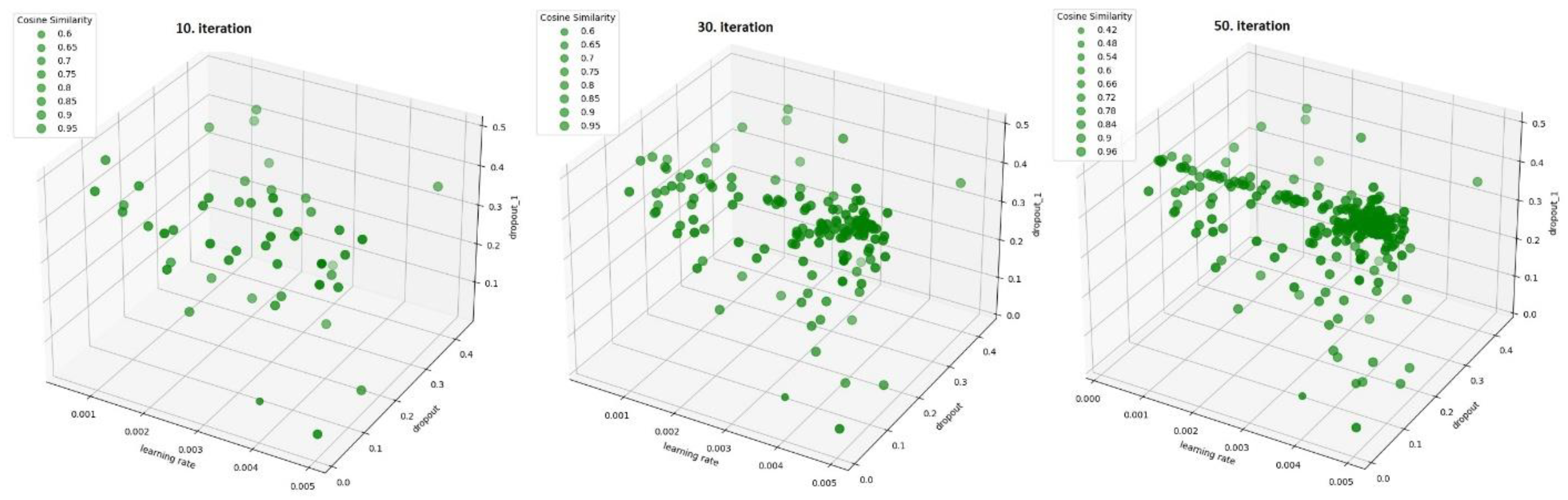
4.3. Hyperparameter Tuning

Hyperparameter tuning was done in three stages. The first and second stage were based on grid search with two parameter types. First type string was used for best combination of ConvLSTM2D activation functions. Second type integer was used for best combination for size and numbers of filters in ConvLSTM2D layers. Third type float was used with Particle Swarm Optimization (PSO) for searching in continuous space values for dropout and dropout_1 from Figure 2, and learning rate value for training.
Two grid searches were performed. The first grid search was done in order to choose the best activation function for ConvLSTM2D layers (one was for output layer activation) and the second grid search was done for recurrent_activation. During testing, we noticed that with “linear” and “ReLu” activation functions in any combination, it is impossible to fit the model because during training, all metrics get NAN values, but in combination with other functions it was possible. The obtained results show that the best combination for model is “linear” function for output activation and “hard_sigmoid” for recurrent_activation with CS = 0.9975, EUCD = 22.8787, and RMSE = 0.0662 for test dataset, Figure 3.
The second grid search was done in order to choose adequate number of filters with filter size for both ConvLSTM2D layers.
In Figure 4, numbers on the X-axis represent the parameters that were examined, e.g., 8, 16, 2, the number eight represents the number of filters in the conv_lst_m2d layer of the model presented in Figure 2. The number 16 represents the number of filters in the conv_lst_m2d_1 layer. The number two represents the square shape filter (kernel) size for both ConvLSTM layers. The best combination was 32,32,3 with metrics CS = 0.9977, EUCD = 22.3570, and RMSE = 0.0648 for test dataset.
The last stage in hyperparameters tuning was PSO, which as a swarm intelligence algorithm was used to find the global minimum of the function with pyswarms Python library [17]. PSO initializes the particle swarm position and velocities from uniform random distribution subject to bounds of the search space, the iterative optimization approach repeats the sequence of steps consisting of (1) calculating traveling velocity dynamically of each particle; (2) updating particle’s personal best value; (3) updating global best value; and (4) updating velocity and positionof each particle in the swarm, until the desired best fitness value or maximum iteration count is met. The update of velocities v and positions x, respectively, is done according to expressions:
v t + 1 = w v i t + c 1 r 1 p i x i t + c 2 r 2 p g x i t
x i t + 1 = x i t + v i t + 1
where pi is the personal best position of the individual particle from previous iterations, pg is the global best position in the swarm from previous iterations, w denotes inertia parameter, c1 is parameter representing cognitive behavior (cognitive coefficient), while c2 influences social behavior (social coefficient), r1 and r2 are random numbers from the unit segment defining stochastic behavior of the algorithm, index i, ranging from 1 to N, where N is the total number of particles, identifies each particle in the swarm and t is the discrete time. These expressions reflect the nature of swarm based metaheuristics in which individual and collective (social) behavior of agents in a swarm leads to complex behavior of the system capable of reaching the desired optimal goal. In this study, five particles were used in 50 iterations, where the set parameters cognitive = 1, social = 2.5, and inertia = 0.3 favoring the social moment of the PSO. The process of searching for optimal values in a three-dimensional continuous space is shown in Figure 5.
As can be noticed from Figure 5, the PSO algorithm randomly searches for parameters in the first ten iterations. From the tenth to the thirtieth iteration grouping near optimal values for “dropout” and “dropout_1” can be noticed. For the last 20 iterations, the PSO algorithm is mainly focused on finding the optimal value for “learning rate”. The optimal values are 0.15649, 0.43055, and 0.00436 for “dropout”, “dropout_1”, and “learning rate”, respectively. For these parameters metrics are CS = 0.9978, EUCD = 21.6647, and RMSE = 0.0632 for test dataset. ConvLSTM-SA model was tested with the fully optimized parameters from hyperparameters tuning.
Another evaluation was performed with cross validation on all images in database. The obtained results are presented in Table 3.
Table 3 shows that the best results are CS = 0.9979, RMSE = 0.0613, and EUCD = 21.1876 for test subset. Based on the defined evaluation criteria from 4.1 Evaluation criteria, the ConvLSTM-SA model is capable of producing a global AOT image and is capable of finding patterns in the time domain.
Table 4 shows statistical results from comparison between ConvLSTM-SA model and reference ConvLSTM model from previous study [3].
From Table 4 it can be concluded that CS metrics has not been changed significantly, but RMSE and EUCD show the best improvements of −13.86% and −7.01%, respectively. The results for the test set should be considered the most objective, and thus the obtained improvements are comparatively 0.03%, −6.06%, and −6.57% for CS, RMSE, and EUCD metrics respectively.

4.4. Ablation Study on Self-Attention Mechanism

In order to evaluate impact and contribution of SA, we removed SA layer from ConvLSTM-SA model. The testing was performed with the same hyperparameters. The cross validation results are given in Table 5.
From Table 5 it can be concluded that the best values are CS = 0.9980 RMSE = 0.0597 and EUCD = 20.7411 for model without SA layer. For better presentation of the results we made Table 6 with statistics for the model with and without SA. Based on the defined evaluation criteria from 4.1 Evaluation criteria, the ConvLSTM-SA model without SA layer, i.e., with ablation, is capable of producing a global AOT image and is capable of finding patterns in the time domain.
The biggest differences are in the test set, such as 0.008%, −2.00%, and −2.02% difference to the ConvLSTM-SA model for CS, RMSE, and EUCD respectively.

4.5. Statistical Tests

In order to better evaluate the SA mechanism with ConvLSTM model for predicting the global AOT image, statistical testing was additionally performed. The statistical testing was done on grayscale images for the sake of simplification, and it was shown that in this way it is possible to statistically compare images of the same content [18]. The first statistical testing refers to obtained images by prediction with ConvLSTM-SA model and by model after remove SA, i.e., without SA layer. This tests the capabilities of the models in terms of the quality of generated images. Another way of testing refers to statistical testing of time series based on pixels. Time series for pixels were obtained based on all the values that one pixel has in the test subset obtained by model prediction. This testing evaluates the model’s ability to recognize changes in the time domain.
Considering that most statistical tests imply that the data being tested have a normal distribution, the first test we performed was testing for the normal distribution of the data. For this test, we used the normaltest method from the scipy.stats library, which is based on skewness and kurtosis metrics [19]. The results of statistical testing are shown in Table 7.
Statistical testing of images was performed by comparing sequences of images, where one sequence represents one horizontal row of pixels. The given results represent the total mean values of the testing, and the 0.05 value was taken as the limit value for the p value [18,20]. As can be seen from Table 7, the assumed hypothesis that the images have a normal distribution is not valid. For this reason, the matching of the sample distribution of the compared images was tested using the Kruskal–Wallis test [21]. The null hypothesis being tested is that images are similar if they have a similar distribution of grayscale samples [18]. Based on the results of this test with the same threshold p value of 0.05, it can be concluded that the model with and without the SA layer generate images similar to those from the original dataset. At the same time, the images generated by the models with and without the SA layer are not similar to each other according to the same criterion. Generated images more similar to the original ones were achieved by the model without the SA layer with p value = 0.0992.
Statistical testing of pixels in the time domain was performed by comparing the series of all achieved values in the test subset for individual grayscale pixels. Neither the original data nor the data obtained by model prediction with SA passed the test of normal distribution with a threshold p value of 0.05. Only the model without SA passed the normality test, so we performed another Kruskal–Wallis test. The null hypothesis being tested is that time series are similar if they have a similar distribution of grayscale samples [18]. The results from Table 7 show that the sequences generated by both models are similar and that the null hypothesis is valid. Additionally, time series predicted by model with and without SA can be considered similar according to the null hypothesis and the threshold value for p values. The data generated by the model without SA showed a good agreement with the original data, reaching p value = 0.2373.
Another study [22] reports a comparative evaluation of bidirectional long short-term memory network with attention layers and their findings suggest that the additional attention layer does not improve upon a less complex approach which is the same as the findings in this study.

5. Conclusions and Future Research

In order to improve the developed ConvLSTM model from previous study, the SA mechanism was implemented. Hyperparameter tuning with grid search and PSO for five particles and 50 iterations enabled better fitting of the model. Model ConvLSTM-SA and model without SA layer was verified with two evaluation criteria which refers that models are able to generate image of the global AOT concentration and it could find patterns in the time domain. ConvLSTM-SA model had better performances than reference model ConvLSTM sequence-to-one. RMSE and EUCD show improvements of −13.86% and −7.01%, respectively.
The ablation study on the SA mechanism showed lower RMSE and EUCD compared to the ConvLSTM-SA model (≈2%). Additionally, statistical comparisons showed that the SA layer did not meet expectations and developed model without SA layer performs better global AOT image prediction. The hypothesis that the grayscale images obtained by the model prediction with and without SA layer belong to a normal distribution is not valid. The grayscale images generated by ConvLSTM-SA model and model without SA layer passed Kruskal–Wallis test where the model without the SA layer had better result with p value = 0.0992. The Kruskal–Wallis test for pixels in the time domain, i.e., time series, was successful for the model with and without SA layer but without was better with p value = 0.2373.
Considering the positive influence of the hyperparameter tuning of the model in future research, the application of this technique to the reference model that was developed and presented in the previous study can be taken into consideration.
The differences between ConvLSTM-SA model with and without SA layer for RMSE and EUCD are −2.00%, and −2.02% for the test subset which indicate that model behaves better without SA layer. Although the obtained results lead to a conclusion that the model without SA layer has better performance, the authors plan to improve the implementation of attention mechanism with the ConvLSTM model by encoder-decoder architecture.

Author Contributions

Conceptualization: D.S.R., D.P.N. and U.R.R.; methodology: D.P.N., D.S.R. and N.S.M.; formal analysis: I.M.L.; investigation: U.R.R. and I.M.L.; writing—review and editing: D.P.N., D.S.R. and N.S.M. All authors have read and agreed to the published version of the manuscript.

Funding

The research was funded by the Ministry of Education, Science and Technological Development of the Republic of Serbia, Contract No. 451-03-47/2023-01/200017.

Data Availability Statement

The study did not report any data.

Acknowledgments

The authors gratefully acknowledge the NASA Earth Observations (NEO) for their effort in making the data available. The authors gratefully acknowledge the support of NVIDIA Corporation with the donation of the Tesla K40c GPU used for this research.

Conflicts of Interest

The authors declare no conflict of interest.

References

  1. Duncan, B.N.; Prados, A.I.; Lamsal, L.N.; Liu, Y.; Streets, D.G.; Gupta, P.; Hilsenrath, E.; Kahn, R.A.; Nielsen, J.E.; Beyersdorf, A.J.; et al. Satellite data of atmospheric pollution for U.S. air quality applications: Examples of applications, summary of data end-user resources, answers to FAQs, and common mistakes to avoid. Atmos. Environ. 2014, 94, 647–662. [Google Scholar] [CrossRef] [Green Version]
  2. Logan, T.; Dong, X.; Xi, B. Aerosol properties and their impacts on surface CCN at the ARM Southern Great Plains site during the 2011 Midlatitude Continental Convective Clouds Experiment. Adv. Atmos. Sci. 2018, 35, 224–233. [Google Scholar] [CrossRef]
  3. Nikezić, D.P.; Ramadani, U.R.; Radivojević, D.S.; Lazović, I.M.; Mirkov, N.S. Deep Learning Model for Global Spatio-Temporal Image Prediction. Mathematics 2022, 10, 3392. [Google Scholar] [CrossRef]
  4. Wangperawong, A. Attending to Mathematical Language with Transformers. arXiv 2019. [Google Scholar] [CrossRef]
  5. Vaswani, A.; Bengio, S.; Brevdo, E.; Chollet, F.; Gomez, A.N.; Gouws, S.; Uszkoreit, J. Tensor2Tensor for Neural Machine Translation, AMTA. In Proceedings of the 13th Conference of the Association for Machine Translation in the Americas, Association for Machine Translation in the Americas, Boston, MA, USA, 17–21 March 2018; Volume 1: Research Track, pp. 193–199. [Google Scholar]
  6. Su, J.; Byeon, W.; Kossaifi, J.; Huang, F.; Kautz, J.; Anandkumar, A. Convolutional Tensor-Train LSTM for Spatio-Temporal Learning. In Proceedings of the Advances in Neural Information Processing Systems 33 (NeurIPS 2020), Virtual, 6–12 December 2020; Volume 33, pp. 13714–13726, ISBN 9781713829546. [Google Scholar]
  7. Zivkovic, M.; Jovanovic, L.; Ivanovic, M.; Bacanin, N.; Strumberger, I.; Joseph, P.M. XGBoost Hyperparameters Tuning by Fitness-Dependent Optimizer for Network Intrusion Detection. In Communication and Intelligent Systems; Sharma, H., Shrivastava, V., Kumari Bharti, K., Wang, L., Eds.; Lecture Notes in Networks and Systems; Springer: Singapore, 2022; Volume 461. [Google Scholar] [CrossRef]
  8. Lin, Z.; Li, M.; Zheng, Z.; Cheng, Y.; Yuan, C. Self-Attention ConvLSTM for Spatiotemporal Prediction. In Proceedings of the Thirty-Fourth AAAI Conference on Artificial Intelligence (AAAI-20), New York, NY, USA, 7–12 February 2020. [Google Scholar] [CrossRef]
  9. Vaswani, A.; Shazeer, N.; Parmar, N.; Uszkoreit, J.; Jones, L.; Gomez, A.N.; Polosukhin, I. Attention Is All You Need. In Proceedings of the Advances in Neural Information Processing Systems 30 (NIPS 2017), Long Beach, CA, USA, 4–9 December 2017; Volume 30, ISBN 9781510860964. [Google Scholar]
  10. Dosovitskiy, A.; Beyer, L.; Kolesnikov, A.; Weissenborn, D.; Zhai, X.; Unterthiner, T.; Houlsby, N. An Image is Worth 16 × 16 Words: Transformers for Image Recognition at Scale. In Proceedings of the International Conference on Learning Representations (ICLR 2021), Vienna, Austria, 4–8 May 2021. [Google Scholar]
  11. Luong, M.-T.; Pham, H.; Manning, C.D. Effective Approaches to Attention-based Neural Machine Translation. In Proceedings of the 2015 Conference on Empirical Methods in Natural Language Processing, Association for Computational Linguistics, Lisbon, Portugal, 17–21 September 2021; pp. 1412–1421. [Google Scholar]
  12. Dzmitry, B.; Cho, K.; Bengio, Y. Neural Machine Translation by Jointly Learning to Align and Translate. arXiv 2016, arXiv:1409.0473. [Google Scholar] [CrossRef]
  13. Khan, S.; Naseer, M.; Hayat, M.; Zamir, S.W.; Khan, F.S.; Shah, M. Transformers in Vision: A Survey. ACM Comput. Surv. 2022, 54, 1–41. [Google Scholar] [CrossRef]
  14. Wensel, J.; Ullah, H.; Munir, A. ViT-ReT: Vision and Recurrent Transformer Neural Networks for Human Activity Recognition in Videos. arXiv 2022, arXiv:2208.07929. [Google Scholar] [CrossRef]
  15. Kaiser, Ł.; Bengio, S. Can Active Memory Replace Attention? In Proceedings of the 30th International Conference on Neural Information Processing Systems (NIPS’16), Barcelona, Spain, 5–10 December 2016; Curran Associates Inc.: Red Hook, NY, USA, 2017; pp. 3781–3789. [Google Scholar]
  16. Ge, H.; Li, S.; Cheng, R.; Chen, Z. Self-Attention ConvLSTM for Spatiotemporal Forecasting of Short-Term Online Car-Hailing Demand. Sustainability 2022, 14, 7371. [Google Scholar] [CrossRef]
  17. Bacanin, N.; Zivkovic, M.; Stoean, C.; Antonijevic, M.; Janicijevic, S.; Sarac, M.; Strumberger, I. Application of Natural Language Processing and Machine Learning Boosted with Swarm Intelligence for Spam Email Filtering. Mathematics 2022, 10, 4173. [Google Scholar] [CrossRef]
  18. Elements of Multivariate Statistics and Statistical Learning, Statistical Image Analysis, Department of Mathematics, Dartmouth College. Available online: https://math.dartmouth.edu/~m70s20/ImageAnalysis.pdf (accessed on 19 January 2023).
  19. D’Agostino, R.B. An omnibus test of normality for moderate and large sample size. Biometrika 1971, 58, 341–348. [Google Scholar] [CrossRef]
  20. Bacanin, N.; Stoean, R.; Zivkovic, M.; Petrovic, A.; Rashid, T.A.; Bezdan, T. Performance of a Novel Chaotic Firefly Algorithm with Enhanced Exploration for Tackling Global Optimization Problems: Application for Dropout Regularization. Mathematics 2021, 9, 2705. [Google Scholar] [CrossRef]
  21. Kruskal, W.H.; Wallis, W.W. Use of Ranks in One-Criterion Variance Analysis. J. Am. Stat. Assoc. 1952, 47, 583–621. [Google Scholar] [CrossRef]
  22. Spliethöver, M.; Klaff, J.; Heuer, H. Is It Worth the Attention? A Comparative Evaluation of Attention Layers for Argument Unit Segmentation. In Proceedings of the 6th Workshop on Argument Mining, Association for Computational Linguistics, Florence, Italy, 1 August 2019; pp. 74–82. [Google Scholar]
Figure 1. Global AOT concentration.
Mathematics 11 01744 g001
Figure 2. Plot of ConvLSTM-SA model for sequence-to-one prediction.
Mathematics 11 01744 g002
Figure 3. Grid search for activation functions through both ConvLSTM2D layers.
Mathematics 11 01744 g003
Figure 4. Grid search for number of filters and filters size.
Mathematics 11 01744 g004
Figure 5. Particle Swarm Optimization for “dropout”, “dropout_1”, and “learning rate”.
Mathematics 11 01744 g005
Table 1. Average difference with STD of AOT database images.
CSRMSEEUCD
1. criterion for evaluation0.9950
±0.002
0.0931
±0.018
32.8803
±6.318
2. criterion for evaluation0.9975
±0.001
0.0663
±0.013
23.3766
±4.493
Table 2. Cross validation with reference model.
RatioTrainValidationTest
CSRMSEEUCDCSRMSEEUCDCSRMSEEUCD
70:20:100.99820.073623.17460.99850.066423.12720.99750.066523.0200
70:10:200.99820.072723.22430.99850.067023.24730.99760.066022.9765
20:70:100.99820.074123.30530.99860.067923.59690.99750.066823.1850
20:10:700.99820.068223.44330.99840.068223.68100.99760.065622.8610
10:70:200.99810.075223.65910.99860.068323.75240.99740.068023.5864
10:20:700.99840.071123.11470.99860.066523.08070.99760.066723.0897
Table 3. Cross validation of ConvLSTM-SA model with self-attention.
RatioTrainValidationTest
CSRMSEEUCDCSRMSEEUCDCSRMSEEUCD
70:20:100.99870.062421.70020.99870.062521.69250.99780.062421.5246
70:10:200.99880.061921.24340.99880.061421.21960.99790.061321.2229
20:70:100.99870.062121.3080.99870.063321.81140.99790.061521.1876
20:10:700.99870.063722.25040.99860.065222.55770.99790.062421.6773
10:70:200.99870.062321.55560.99880.062321.57170.99780.063321.7486
10:20:700.99870.06322.0450.99870.063622.07640.99770.064522.2383
Table 4. Statistical comparison between ConvLSTM-SA model and reference ConvLSTM model.
CSRMSEEUCD
AVGDIFF [%]AVGDIFF [%]AVGDIFF [%]
Train0.99872
±4 × 10⁻³%
5 × 10⁻²
±1 × 10⁻²
6.25 × 10⁻²
±1.07%
−13.86
±3.63
21.68
±1.85%
−7.01
±2.04
Validation0.99872
±7.5 × 10⁻³%
1.8 × 10⁻²
±1.1 × 10⁻²
6.3 × 10⁻²
±2.08%
−6.43
±2.44
21.82
±2.10%
−6.80
±2.45
Test0.99783
±8.2 × 10⁻³%
3 × 10⁻²
±1.2 × 10⁻²
6.3 × 10⁻²
±1.9%
−6.06
±2.27
21.60
1.80%
−6.57
±2.10
Table 5. Cross validation for ablation study of the ConvLSTM-SA model.
RatioTrainValidationTest
CSRMSEEUCDCSRMSEEUCDCSRMSEEUCD
70:20:100.99870.063421.48300.99880.061921.46710.99790.061721.2680
70:10:200.99870.062721.28720.99880.061721.30750.99790.061021.1572
20:70:100.99880.061821.13370.99880.062521.58100.99790.061121.0578
20:10:700.99870.062421.37610.99870.062921.73070.99800.059720.7411
10:70:200.99870.062621.29600.99880.061721.32590.99790.062221.3959
10:20:700.99870.062221.22850.99880.061321.23810.99790.062221.3617
Table 6. Statistical comparison between ConvLSTM-SA model and model without self-attention layer.
CSRMSEEUCD
AVGDIFF [%]AVGDIFF [%]AVGDIFF [%]
Train0.99872
±4.1 × 10⁻³%
0
±5.8 × 10⁻³
6.25 × 10⁻²
±0.86%
−7.99 × 10⁻²
±1.37
21.30
±0.56%
−1.77
±1.93
Validation0.99878
±4.0 × 10⁻³%
6.7 × 10⁻³
±8.5 × 10⁻³
6.2 × 10⁻²
±0.95%
−1.67
±2.28
21.44
±0.87%
−1.74
±2.27
Test0.99792
±4.0 × 10⁻³%
8.4 × 10⁻³
±9.1 × 10⁻³
6.1 × 10⁻²
±1.54%
−2.00
±2.45
21.16
±1.15%
−2.02
±2.13
Table 7. Results of statistical testing for predicted images and pixels in the time domain for the test subset.
Object of TestingSort of TestingDataStatisticp Value
ImageNormaltestoriginal312.740.0156
ConvLSTM-SA323.480.0033
ConvLSTM187.110.0230
Kruskal–Wallis
H test
Original/ConvLSTM-SA161.850.0823
Original/ConvLSTM119.560.0992
ConvLSTM-SA/ConvLSTM151.820.0444
Pixel in time domainNormaltestoriginal137.120.0377
ConvLSTM-SA55.340.0198
ConvLSTM63.160.0537
Kruskal–Wallis
H test
Original/ConvLSTM-SA52.040.0927
Original/ConvLSTM29.800.2373
ConvLSTM-SA/ConvLSTM54.760.0848
Disclaimer/Publisher’s Note: The statements, opinions and data contained in all publications are solely those of the individual author(s) and contributor(s) and not of MDPI and/or the editor(s). MDPI and/or the editor(s) disclaim responsibility for any injury to people or property resulting from any ideas, methods, instructions or products referred to in the content.

