Gain Scheduled Fault Detection Filter for Markovian Jump Linear System with Nonhomogeneous Markov Chain

Abstract

In a networked control system scenario, the packet dropout is usually modeled by a time-invariant (homogeneous) Markov chain (MC) process. However, from a practical point of view, the probabilities of packet loss can vary in time and/or probability parameter dependency. Therefore, to design a fault detection filter (FDF) implemented in a semi-reliable communication network, it is important to consider the variation in time of the network parameters, by assuming the more accurate scenario provided by a nonhomogeneous jump system. Such a premise can be properly taken into account within the linear parameter varying (LPV) framework. In this sense, this paper proposes a new design method of ${\mathcal{H}}_{\infty }$ gain-scheduled FDF for Markov jump linear systems under the assumption of a nonhomogeneous MC. To illustrate the applicability of the theoretical solution, a numerical simulation is presented.

1. Introduction

In order to keep a manufacturing process as lean as possible, there are several aspects that must be considered. The monitoring capability is one of the features receiving the major spotlight in industrial operations since it is crucial to guarantee that the process is safe for the personnel involved. Among the procedures that constitute the monitoring systems, one that is worth mentioning is the fault-detection (FD) process [1,2].

A fault can be seen as the first indication of more harsh problems. It is any type of unwanted minor behavior that was not expected from the system. It can be caused, for instance, by extended wear due to long periods of time without maintenance. As a consequence of inadequately fixed wear, malfunctions or failures can cause a breakage [3].

In this sense, FD is a model-based process in which any abnormal/unexpected behavior is detected by a two-step procedure. The first step in the FD process is the residue generation, performed by an observer. The second step is the evaluation process, where the residue signal, generated by the observer, is treated by an evaluation function and compared with a predetermined threshold. We assume that a fault has occurred if the evaluation function surpasses the threshold; otherwise, we consider that the system is working as intended [4].

Currently, an important assumption that must be taken into account in FD systems is that the communication between the components is made via semireliable networks, which are associated with occasional packet dropout. These dropouts are caused by different sources as package collision due to high network congestion [5]. The distinction between a dropout and a fault is an essential aspect of the FD process since it makes easier to locate a fault. A viable way to model a packet dropout in a network is to employ a Markov jump linear system (MJLS) framework. This representation is appropriate to handle systems whose dynamic behavior is subject to random abrupt changes, like those caused by network packet dropouts. In this scenario, a Markov chain (MC) is used to model the jumping between the modes of operation of the system [6].

In the literature, there are plenty of examples of FD approaches that consider network behavior in their design. For instance, in [7,8] linear matrix inequality (LMI)-based constraints are provided to design fault detection filters (FDF) by using the ${\mathcal{H}}_{\infty }$ norm as a performance index. In [9], the authors have developed an FD approach for underactuated manipulators modeled by MJLS. In [10], an FD method for networked control systems (NCS) under the assumption of the existence of a variable delay between the signals received by the system components is tackled. In [11], a fault detection filter under the MJLS formulation was applied to a control moment gyroscope. In [12], a fault-detection filtering problem is tackled under the Markov switching memristive neural networks. In [13], an observed-based sliding mode control problem based on the event-triggered protocol under the Markovian jump systems framework was presented. In [14], a fault-detection filter for discrete time Markov jump Lur’e systems with bounded sector condition. Observing all the above examples, one fundamental premise in the MJLS context is that the Markov chain (MC) is considered to be homogeneous [15], which means that it does not vary in time. However, since the packet dropout sources (collision, congestion, networked-induced delay) change in time, we consider that a fixed transition probability between the Markovian operation modes does not properly model the network behavior. A way to handle the particularity of a time-varying MC was presented in [16], where the author has proposed new LMI constraints to evaluate the stability of MJLS governed by a nonhomogeneous MC. A particular case of the proposal presented by [16], which allows for designing FDF for MJLS systems affected by nonhomogeneous MCs, consists of using a linear parameter varying (LPV)-based representation for the time-varying transition probability matrix [17,18]. There are several works in the literature that deal with the problem of control (or filter) synthesis for nonlinear systems by using different approaches. For example, regarding the design of fault-tolerant controllers, there are strategies based on fuzzy systems [19] capable of modeling system nonlinearities by using Takagi–Sugeno models, so that if the probability of actuator failure is small, the control mode is normal, and if the probability is high, the control is changed to fault-tolerant mode. Another strategy to deal with nonlinearities that can be found in the literature arises in the context of sliding mode control [20]. In this case, the class of discrete-time nonlinear systems with delays and uncertainties that is considered is the conic type, where the nonlinear terms satisfy the constraint that lies in a known hypersphere with an uncertain center. However, the proposed approach, in addition to considering the loss of packets in the communication network via the Markov chain, deals with the nonlinearity of the systems by using a different strategy from those previously discussed, in which the modes of operation are considered linear but depend on time-varying parameters. Such modeling allows the use of convex optimization methods and LMI-based tools to solve the filtering problem without adding extra levels of complexity.

In view of the above works, the main contribution of the present work are

• the proposition of a new design technique of gain-scheduled FDF for MJLS with nonhomogeneous MC, and
• the numerical simulation to reinforce the usability of the proposed theoretical solution.

The proposed approach describes the nonhomogeneous MC using linear time-varying parameters to model those variations, assuming that these parameters are known or at least measurable. Another important assumption made is that the probability varies in time arbitrarily. Hence, the probability parameter for the following instant $(k+1)$ does not depend on present instant k, which grants the ability to disassociate the Lyapunov function in two distinct simplexes. Based on this assumption, we propose the design of a gain-scheduled fault-detection filter where the scheduling parameter implemented is the one that dictates the variation of the MC. One advantage of the proposed approach, when compared with others found in the literature, is that the design conditions assure the system stability for the entire parameter-varying range since the FDF is scheduled in terms of time-varying parameters modeling the network variation. The major novelty of the proposed technique is the higher level of fidelity in the representation of the network influence in the system model. Since FD is a model-based approach, a more accurate representation of the system can lead to better performance in practice.

The paper is organized as follows. Section 2 and Section 4 present the necessary theoretical fundamentals. Section 3 shows how to model the nonhomogeneous Markov Chain by using LPV. Section 5 introduces the problem formulation and the main contributions. Section 6 illustrates the feasibility of applying the proposed technique, by means of a numerical simulation, and Section 7 concludes the paper with some final remarks.

Notation

The real Euclidean space is denoted by ${\mathbb{R}}^n$ where n represents its dimension and a real matrix with n rows and m columns is represented by ${\mathbb{R}}^{n\times m}$. The symbol $I_n$ stands for an $n\times n$ identity matrix (or, for simplicity, just I, with an appropriate dimension, whenever no confusion arises) and the symbol ${\left(·\right)}^{\prime }$ denotes the transpose of a matrix. The operator $\mathrm{Her}\left(·\right)$ is used to express the symmetric sum as in $\mathrm{Her}\left(X\right)=X+X^{\prime }$, while the operator $\mathrm{diag}\left(·\right)$ represents a diagonal matrix. The symbol • denotes a symmetric block in a partitioned symmetric matrix. The expected value operator is represented by $\mathbb{E}\left(·\right)$ and the conditional expected operator is denoted by $\mathbb{E}\left(·\right|·)$. The fundamental probability space is described by $(\Omega ,\mathcal{F},\left\{{\mathcal{F}}_k\right\},Pr\left(·\right))$. The space ${\mathcal{L}}^2$ is the Hilbert space formed by ${\mathcal{F}}_k$-measurable random sequences ${\left\{z_k\right\}}_{k=0}^{\infty }$ such that ${\parallel z\parallel }_2\triangleq {\left[{\sum }_{k=0}^{\infty }{\mathbb{E}\left\{\right|z\left(k\right)|}^2\}\right]}^{1/2}<\infty$.

2. Preliminaries

A generic discrete-time MJLS is given by

$$\mathcal{G}\equiv \left\{\begin{array}{c}\hfill x(k+1)=A_{{\theta }_k}x\left(k\right)+J_{{\theta }_k}w\left(k\right)\\ \hfill z\left(k\right)=C_{{\theta }_k}x\left(k\right)+D_{{\theta }_k}w\left(k\right)\end{array},\right.$$

(1)

where $x\left(k\right)\in {\mathbb{R}}^{n_x}$ is for the state vector, $w\left(k\right)\in {\mathbb{R}}^{n_w}$ is the exogenous input vector, and $z\left(k\right)\in {\mathbb{R}}^{n_z}$ is the output signal. The state-space matrices of system (1) depend on the index ${\theta }_k$, which represents a discrete-time Markov chain belonging to a finite set of modes $\mathbb{K}=\{1,\cdots ,\sigma \}$, whose switching is ruled by a time-varying transition probability matrix

$$\begin{array}{c}\hfill \mathbb{P}\left(k\right)=\left[\begin{array}{ccc}{\rho }_{11}\left(k\right)& \cdots & {\rho }_{1\sigma }\left(k\right)\\ & \ddots & \\ {\rho }_{\sigma 1}\left(k\right)& \cdots & {\rho }_{\sigma \sigma }\left(k\right)\end{array}\right].\end{array}$$

(2)

The entries ${\rho }_{ij}\left(k\right)$ of $\mathbb{P}\left(k\right)$ are such that ${\rho }_{ij}\left(k\right)=\mathrm{Pr}({\theta }_{k+1}=j|{\theta }_k=i),\forall k\ge 0$, ${\rho }_{ij}\left(k\right)\ge 0$, and ${\sum }_{j=1}^{\sigma }{\rho }_{ij}\left(k\right)=1$. We recall that whenever the transition matrix is time-invariant, that is, $\mathbb{P}\left(k\right)=\mathbb{P}$, the associated Markov chain is said to be homogeneous; otherwise, it is called nonhomogeneous (meaning that the probabilities vary in time) [15,21]. It is assumed that ${\rho }_{ij}\left(k\right)$ varies within the following interval: $0\le {\underline{\rho }}_{ij}\le {\rho }_{ij}\left(k\right)\le {\overline{\rho }}_{ij}\le 1$, where ${\underline{\rho }}_{ij}$ represents lower bound and ${\overline{\rho }}_{ij}$ denotes the upper bound. Another important assumption is that the upper and lower bounds of the transition probability are known, and the transition probability variation is instantly measurable. Therefore, all the parameters in (2) may vary in a known range with ${\rho }_{ij}\left(k\right)\in [{\underline{\rho }}_{ij},{\overline{\rho }}_{ij}]$. There are several ways to determine the values of the upper (${\overline{\rho }}_{ij}$) and lower (${\underline{\rho }}_{ij}$) bounds of ${\rho }_{ij}\left(k\right)$. Those values can be obtained via mathematical modeling, observation, estimation, simulation, or based on the a priori knowledge of the system, such that the estimate can vary among systems and depends on the type of variation to which the system is subjected.

From the constraints ${\sum }_{j=1}^{\sigma }{\rho }_{ij}\left(k\right)=1$ and $0\le {\underline{\rho }}_{ij}\le {\rho }_{ij}\left(k\right)\le {\overline{\rho }}_{ij}\le 1$, the transition matrix (2) can be described by N polytopic intervals, where N depends on the number of transition probabilities that are time-varying. From these polytopic intervals, some techniques can be applied to obtain a gain-scheduled FDF.

In order to exemplify these N polytopic intervals and how to define a time-varying transition matrix by using LPV, let us assume that $\sigma =5$ and the parameters ${\rho }_{14}\left(k\right)$ and ${\rho }_{15}\left(k\right)$ vary in time; hence, the first row of the transition matrix (2) can be written as

$$\begin{array}{c}\hfill \left[\begin{array}{ccccc}{\rho }_{11}& {\rho }_{12}& {\rho }_{13}& {\rho }_{14}\left(k\right)& {\rho }_{15}\left(k\right)\end{array}\right],\end{array}$$

(3)

and from this row, two polytopic intervals ($N=2$) are obtained:

$$\begin{array}{c}\hfill \left[\begin{array}{ccccc}{\rho }_{11}& {\rho }_{12}& {\rho }_{13}& {\underline{\rho }}_{14}& {\overline{\rho }}_{15}\end{array}\right],\left[\begin{array}{ccccc}{\rho }_{11}& {\rho }_{12}& {\rho }_{13}& {\overline{\rho }}_{14}& {\underline{\rho }}_{15}\end{array}\right].\end{array}$$

(4)

The polytopic intervals obey the constraints ${\sum }_{j=1}^{\sigma }{\rho }_{ij}\left(k\right)=1$ and $0\le {\underline{\rho }}_{ij}\le {\rho }_{ij}\left(k\right)\le {\overline{\rho }}_{ij}\le 1$ simultaneously. The following notation will be used to represent a time-varying row of $\mathbb{P}\left(k\right)$ as in (3) with the lower and upper bounds as in (4):

$$\begin{array}{c}\hfill \left[\begin{array}{ccccc}{\rho }_{11}& {\rho }_{12}& {\rho }_{13}& [{\underline{\rho }}_{14},{\overline{\rho }}_{14}]& [{\underline{\rho }}_{15},{\overline{\rho }}_{15}]\end{array}\right].\end{array}$$

(5)

The main novelty in this paper is the usage of the same time-varying parameters that coordinate the nonhomogeneous MC variation as gain-scheduled parameters for the design and implementation of the FDF. This concept will be carefully described in Section 3.

Although the time variation that affects the probability matrix is generally represented by modeling $\mathbb{P}\left(k\right)$ as belonging to a polytope, in this paper we choose to use another approach, which describes each time-varying row of $\mathbb{P}\left(k\right)$ in terms of a linear time-varying parameter vector ${\alpha }_r\left(k\right)$ belonging to a distinct unit simplex ${\mathrm{\Lambda }}_{N_r}$, $r=1,2,\cdots ,m$. The definition of the unit simplex is given by

$$\begin{array}{c}\hfill {\mathrm{\Lambda }}_{N_r}\equiv \left\{\zeta \in {\mathbb{R}}^{N_r}|\sum _{i=1}^{N_r}{\zeta }_i=1,{\zeta }_i\ge 0,i=0,1,\cdots ,N_r\right\},\end{array}$$

(6)

where m is the number of time-varying rows in the probability matrix. In order to group up all the time-varying parameters of $\mathbb{P}\left(k\right)$ in a single domain, we perform a Cartesian product of m simplexes, each one of dimension $N_r$, in a single domain called multisimplex, and represent it by ${\mathrm{\Lambda }}_N={\mathrm{\Lambda }}_{N_1}\times {\mathrm{\Lambda }}_{N_2}\times \cdots \times {\mathrm{\Lambda }}_{N_m}$, with the index N given by $N=(N_1,\dots ,N_m)$. For ease of notation ${\mathbb{R}}^N$ represents the space ${\mathbb{R}}^{N_1+N_2+\dots +N_m}$. In this sense, a given element $\alpha \left(k\right)\in {\mathrm{\Lambda }}_N$ is a vector belonging to ${\mathbb{R}}^N$ and can be decomposed as (${\alpha }_1\left(k\right),{\alpha }_2\left(k\right),\dots ,{\alpha }_m\left(k\right)$) according to the structure of ${\mathrm{\Lambda }}_N$. Subsequently, each ${\alpha }_r\left(k\right)\in {\mathrm{\Lambda }}_r\subset {\mathbb{R}}^{N_r}$, $r=1,\dots ,m$, is decomposed in the form (${\alpha }_{r1},{\alpha }_{r2},\dots ,{\alpha }_{r{N}_r}$). This approach follows the one adopted in [22].

Hereafter, the transition probability will be denoted by ${\rho }_{ij}\left(\alpha \left(k\right)\right)$, where the term $\alpha \left(k\right)\in {\mathrm{\Lambda }}_N$ represents the time-varying parameter responsible to model the probability of the nonhomogeneous Markov chain at time k.

3. Modeling the Nonhomogeneous Markov Chain by Using the Linear Parameter Varying Approach

We next present the definition of a matrix $O_i\left({\iota }_k\right)$, where i represents the MC mode, and ${\iota }_k=({\iota }_1\left(k\right),\dots ,{\iota }_m\left(k\right))$ denotes a generic LPV parameter. It is assumed that $O_i\left({\iota }_k\right)$ is affinely dependent on the time-varying parameters ${\iota }_j\left(k\right)$, as described below:

$$\begin{array}{c}\hfill O_i\left({\iota }_k\right)=O_{i_{{\iota }_0}}+\sum _{j=1}^m{\iota }_j\left(k\right)O_{i_{{\iota }_j}}.\end{array}$$

(7)

The matrix in the affine form (7) can be interpreted in the following manner: matrix ${O_i}_{\iota 0}$ represents the time-invariant part of the filter dynamics. The remaining matrices ${O_i}_{{\iota }_j}$, $j=1,\dots m$ denote the time-varying dynamic that depends on the parameters ${\iota }_j\left(k\right)$. To illustrate this particular structure, consider the example presented below, for an MJLS with three operation modes, whose time-varying probability matrix is given by

$$\begin{array}{c}\hfill \mathbb{P}\left(k\right)=\left[\begin{array}{ccc}0.5& [0.1,0.3]& [0.2,0.4]\\ [0,0.4]& [0.5,0.9]& 0.1\\ 0.2& 0.6& 0.2\end{array}\right],\end{array}$$

(8)

where elements ${\rho }_{12}\left(k\right)$, ${\rho }_{13}\left(k\right)$, ${\rho }_{21}\left(k\right)$ and ${\rho }_{22}\left(k\right)$ vary in a known interval $[{\underline{\rho }}_{ij},{\overline{\rho }}_{ij}]$. Since each uncertain row of $\mathbb{P}\left(k\right)$ can be represented by a polytopic interval, the representation of the first row is given by

$$\begin{array}{c}\hfill \left[\begin{array}{ccc}0.5& 0.1& 0.4\end{array}\right]{\alpha }_{11}\left(k\right)+\left[\begin{array}{ccc}0.5& 0.3& 0.2\end{array}\right]{\alpha }_{12}\left(k\right)\end{array}$$

(9)

and the second row is

$$\begin{array}{c}\hfill \left[\begin{array}{ccc}0& 0.9& 0.1\end{array}\right]{\alpha }_{21}\left(k\right)+\left[\begin{array}{ccc}0.4& 0.5& 0.1\end{array}\right]{\alpha }_{22}\left(k\right)\end{array}$$

(10)

with ${\alpha }_1\left(k\right)=({\alpha }_{11}\left(k\right),{\alpha }_{12}\left(k\right))\in {\mathrm{\Lambda }}_2$, ${\alpha }_2\left(k\right)=({\alpha }_{21}\left(k\right),{\alpha }_{22}\left(k\right))\in {\mathrm{\Lambda }}_2$, and $\alpha \left(k\right)=({\alpha }_1\left(k\right),{\alpha }_2\left(k\right))\in {\mathrm{\Lambda }}_2\times {\mathrm{\Lambda }}_2$. On the other hand, the representation of $\mathbb{P}\left(k\right)$, in terms of parameter $\iota \left(k\right)$ used in the affine structure, can be done as follows,

$$\begin{array}{c}\hfill \mathbb{P}\left(k\right)=\underset{{\mathbb{P}}_{{\iota }_0}}{\underbrace{\left[\begin{array}{ccc}0.5& 0.2& 0.3\\ 0.2& 0.7& 0.1\\ 0.2& 0.6& 0.2\end{array}\right]}}+\underset{{\mathbb{P}}_{{\iota }_1}}{\underbrace{\left[\begin{array}{ccc}0& 1& -1\\ 0& 0& 0\\ 0& 0& 0\end{array}\right]}}{\iota }_1\left(k\right)+\underset{{\mathbb{P}}_{{\iota }_2}}{\underbrace{\left[\begin{array}{ccc}0& 0& 0\\ 1& -1& 0\\ 0& 0& 0\end{array}\right]}}{\iota }_2\left(k\right),\end{array}$$

(11)

where ${\iota }_1\left(k\right)\in [-0.1,0.1]$ and ${\iota }_2\left(k\right)\in [-0.2,0.2]$. Although the modeling seems to be different, note that a simple change of variables can recover the multisimplex modeling from the affine representation, since

$$\begin{array}{c}\hfill {\iota }_r\left(k\right)=\underline{{\iota }_r}{\alpha }_{r1}\left(k\right)+\overline{{\iota }_r}{\alpha }_{r2}\left(k\right),\end{array}$$

(12)

where ${\iota }_r\left(k\right)\in [{\underline{\iota }}_r,{\overline{\iota }}_r]$, ${\alpha }_r\left(k\right)=({\alpha }_{r1}\left(k\right),{\alpha }_{r2}\left(k\right))\in {\mathrm{\Lambda }}_2$, $r=1,2$.

In order to clarify how to write a time-varying matrix in the affine form, consider the following affine matrix as

$$\underset{O_i\left({\iota }_j\right)}{\underbrace{\left[\begin{array}{cc}5& 0.3+{\iota }_1\left(k\right)\\ 12& -2+0.5{\iota }_2\left(k\right)\end{array}\right]}}=\underset{{O_i}_{{\iota }_0}}{\underbrace{\left[\begin{array}{cc}5& 0.3\\ 12& -2\end{array}\right]}}+\underset{{O_i}_{{\iota }_1}}{\underbrace{\left[\begin{array}{cc}0& 1\\ 0& 0\end{array}\right]}}{\iota }_1\left(k\right)+\underset{{O_i}_{{\iota }_2}}{\underbrace{\left[\begin{array}{cc}0& 0\\ 0& 0.5\end{array}\right]}}{\iota }_2\left(k\right),$$

(13)

where ${\iota }_1\left(k\right)\in [\underline{{\iota }_1},\overline{{\iota }_1}]$ and ${\iota }_2\left(k\right)\in [\underline{{\iota }_2},\overline{{\iota }_2}]$. By using the multisimplex formulation, ${\iota }_r\left(k\right)=\underline{{\iota }_r}{\alpha }_{r1}\left(k\right)+\overline{{\iota }_r}{\alpha }_{r2}\left(k\right)$ for $r=1,2$, we recover the representation with $\alpha \left(k\right)\in {\mathrm{\Lambda }}_N={\mathrm{\Lambda }}_2\times {\mathrm{\Lambda }}_2$, where $N=(2,2)$. This procedure can be extended for all matrices throughout this paper. Bearing this in mind, in what follows, whenever we write $P_i\left(\alpha \left(k\right)\right)$ for $\alpha \left(k\right)\in {\mathrm{\Lambda }}_N$, we mean a representation, as in (7), in terms of generic LPV parameters or, equivalently, in terms the multisimplex parameter $\alpha \left(k\right)$.

4. Bounded Real Lemma

The concept of stability for the nonhomogeneous Markov chain is different from its homogeneous counterpart. This discrepancy is caused by the arbitrary variation of the transition probability. Therefore, an upper bound of the ${\mathcal{H}}_{\infty }$ norm can only be obtained if system (1) under the assumption of $w\left(k\right)\equiv 0$ is exponentially stable in the mean square sense with conditioning of type I (ESMS-CI). This concept was first introduced in [23] and is also presented in [16]. In this sense, before introducing the main results of this paper, some fundamental definitions are presented next.

Definition 1 

([16]). Assuming that system (1) is ESMS-CI, and $x\left(0\right)=0$, its ${\mathcal{H}}_{\infty }$ norm is given by

$$\begin{array}{c}\hfill {\parallel \mathcal{G}\parallel }_{\infty }=\underset{w\in {\mathcal{L},\parallel w\parallel }_2\ne o}{sup}\frac{{\parallel z\parallel }_2}{{\parallel w\parallel }_2}.\end{array}$$

(14)

Next, we present a sufficient condition version of the bounded real lemma adapted from [16], which allows us to deal with nonhomogeneous MJLS with arbitrarily fast time-varying parameters, where the parameters are modeled by using the multisimplex domain ${\mathrm{\Lambda }}_N$. For that, it is assumed that the condition $H_1$ in Proposition 1 in [16] is satisfied; that is, $Pr({\theta }_k=i)>0$ for all $i\in \mathbb{K}$ and $k\ge 0$.

Remark 1. 

In order to draw the results presented in Lemma 1, it is necessary to consider the assumption that the variation of the probabilities ${\rho }_{ij}\left(k\right)$ is arbitrarily fast. Under this assumption, there is no need to bound the variation limit.

Lemma 1. 

System (1) is ESMS-CI and satisfies ${\parallel \mathcal{G}\parallel }_{\infty }<\gamma$ if there exist symmetric positive definite matrices $P_i\left(\alpha \left(k\right)\right)$, such that, for each $i\in \mathbb{K}$ and for all $\alpha \left(k\right),\alpha (k+1)\in {\mathrm{\Lambda }}_N$, the parameter-dependent LMIs

$$\begin{array}{c}\hfill \underset{{\Omega }_i\left(\alpha \left(k\right)\right)}{\underbrace{{\left[\begin{array}{cc}{A}_i& J_i\\ C_i& D_i\end{array}\right]}^{\prime }\left[\begin{array}{cc}{\mathbb{E}}_i\left(P\right)(\alpha \left(k\right),\alpha (k+1))& 0\\ 0& I\end{array}\right]\left[\begin{array}{cc}{A}_i& J_i\\ C_i& D_i\end{array}\right]-\left[\begin{array}{cc}{P}_i\left(\alpha \left(k\right)\right)& 0\\ 0& {\gamma }^{2}I\end{array}\right]}}<0\end{array}$$

(15)

are satisfied, where ${\mathbb{E}}_i\left(P\right)(\alpha \left(k\right),\alpha (k+1))={\sum }_{j=1}^{\sigma }{\rho }_{ij}\left(\alpha \left(k\right)\right)P_j\left(\alpha (k+1)\right).$

Proof. 

Here is a sketch of the proof for Lemma 1. Assuming that there exist $P_i\left(\alpha \left(k\right)\right)=P_i^{\prime }\left(\alpha \left(k\right)\right)$ such that Equation (15) holds, we have, from Proposition 1 in [16], that system (1) is ESMSC1. Define the cost function as

$$\begin{array}{c}\hfill {\mathcal{J}}_{\tau }^{\gamma }=\sum _{k=0}^{\tau }E\left[z{\left(k\right)}^{\prime }z\left(k\right)-{\gamma }^{2}w{\left(k\right)}^{\prime }w\left(k\right)\right].\end{array}$$

(16)

Observe that ${\parallel \mathcal{G}\parallel }_{\infty }<\gamma \iff {\mathcal{J}}_{\infty }^{\gamma }\le -e^2{\parallel w\parallel }_2^2,$${\forall \parallel w\parallel }_2\ne 0$ and for some $e\ne 0$, where ${\mathcal{J}}_{\infty }^{\gamma }$ represent the cost function for $\tau \to \infty$. Considering the Lyapunov function ${\mathcal{V}}_{{\theta }_k}(k,x\left(k\right))\triangleq x{\left(k\right)}^{\prime }{P}_{{\theta }_k}\left(\alpha \left(k\right)\right)x\left(k\right)$, one has

$$\begin{array}{cc}\hfill {\mathcal{J}}_{\tau }^{\gamma }=& \sum _{k=0}^{\tau }E\left[z{\left(k\right)}^{\prime }z\left(k\right)-{\gamma }^{2}w{\left(k\right)}^{\prime }w\left(k\right)-{\mathcal{V}}_{{\theta }_k}(k,x\left(k\right))+{\mathcal{V}}_{{\theta }_{k+1}}(k+1,x(k+1))\right]\hfill \\ \hfill & +\sum _{k=0}^{\tau }E\left[{\mathcal{V}}_{{\theta }_k}(k,x\left(k\right))-{\mathcal{V}}_{{\theta }_{k+1}}(k+1,x(k+1))\right]\hfill \\ \hfill =& \sum _{k=0}^{\tau }E\left[z{\left(k\right)}^{\prime }z\left(k\right)-{\gamma }^{2}w{\left(k\right)}^{\prime }w\left(k\right)-{\mathcal{V}}_{{\theta }_k}(k,x\left(k\right))\right]\hfill \\ \hfill & +\sum _{k=0}^{\tau }E\left[E\left[{\mathcal{V}}_{{\theta }_{k+1}}(k+1,x(k+1))|{\mathcal{F}}_k\right]\right]\hfill \\ \hfill & -E\left[{\mathcal{V}}_{\tau +1}(\tau +1,x(\tau +1)\right]+E\left[{\mathcal{V}}_{{\theta }_0}(0,x\left(0\right))\right]\hfill \\ \hfill =& \sum _{k=0}^{\tau }E\left[z{\left(k\right)}^{\prime }z\left(k\right)-{\gamma }^{2}w{\left(k\right)}^{\prime }w\left(k\right)-{\mathcal{V}}_{{\theta }_k}(k,x\left(k\right))\right]\hfill \\ \hfill & +\sum _{k=0}^{\tau }E\left[x{(k+1)}^{\prime }E\left[P_{{\theta }_{k+1}}\left(\alpha (k+1)\right)|{\mathcal{F}}_k\right]x(k+1)\right]\hfill \\ \hfill & -E\left[{\mathcal{V}}_{\tau +1}(\tau +1,x(\tau +1))\right]+E\left[{\mathcal{V}}_{{\theta }_0}(0,x\left(0\right))\right]\hfill \\ \hfill =& \sum _{k=0}^{\tau }E\left[\left[x{\left(k\right)}^{\prime }w{\left(k\right)}^{\prime }\right]{\Omega }_{{\theta }_k}\left(\alpha \left(k\right)\right){\left[x{\left(k\right)}^{\prime }w{\left(k\right)}^{\prime }\right]}^{\prime }\right]\hfill \\ \hfill & -E\left[{\mathcal{V}}_{\tau +1}(\tau +1,x(\tau +1))\right]+E\left[{\mathcal{V}}_{{\theta }_0}(0,x\left(0\right))\right],\hfill \end{array}$$

where ${\Omega }_i\left(\alpha \left(k\right)\right)$ is presented in Equation (15). Recalling that $x\left(0\right)=0$ so that ${\mathcal{V}}_{{\theta }_0}(0,x\left(0\right))=0$, we have $\forall k\ge 0$ and some $e\ne 0$ that

$$\begin{array}{c}\hfill {\mathcal{J}}_{\tau }^{\gamma }=\sum _{k=0}^{\tau }E\left[\left[x{\left(k\right)}^{\prime }w{\left(k\right)}^{\prime }\right]{\Omega }_{{\theta }_k}\left(\alpha \left(k\right)\right)•\right]-E\left[{\mathcal{V}}_{{\theta }_{\tau +1}}(\tau +1,x(\tau +1))\right]\\ \hfill \le \sum _{k=0}^{\tau }E\left[\left[x{\left(k\right)}^{\prime }w{\left(k\right)}^{\prime }\right]{\Omega }_{{\theta }_k}\left(\alpha \left(k\right)\right)•\right]\le -\sum _{k=0}^{\tau }{e}^2{E[\parallel w\left(k\right)\parallel }^2].\end{array}$$

(17)

Inequality (17) yields, as $\tau \to \infty$, that ${\mathcal{J}}_{\infty }^{\gamma }\le -e^2{\parallel w\parallel }_2^2\forall {\parallel w\parallel }_2\ne 0$, showing the desired result.    □

5. Problem Formulation and Main Result

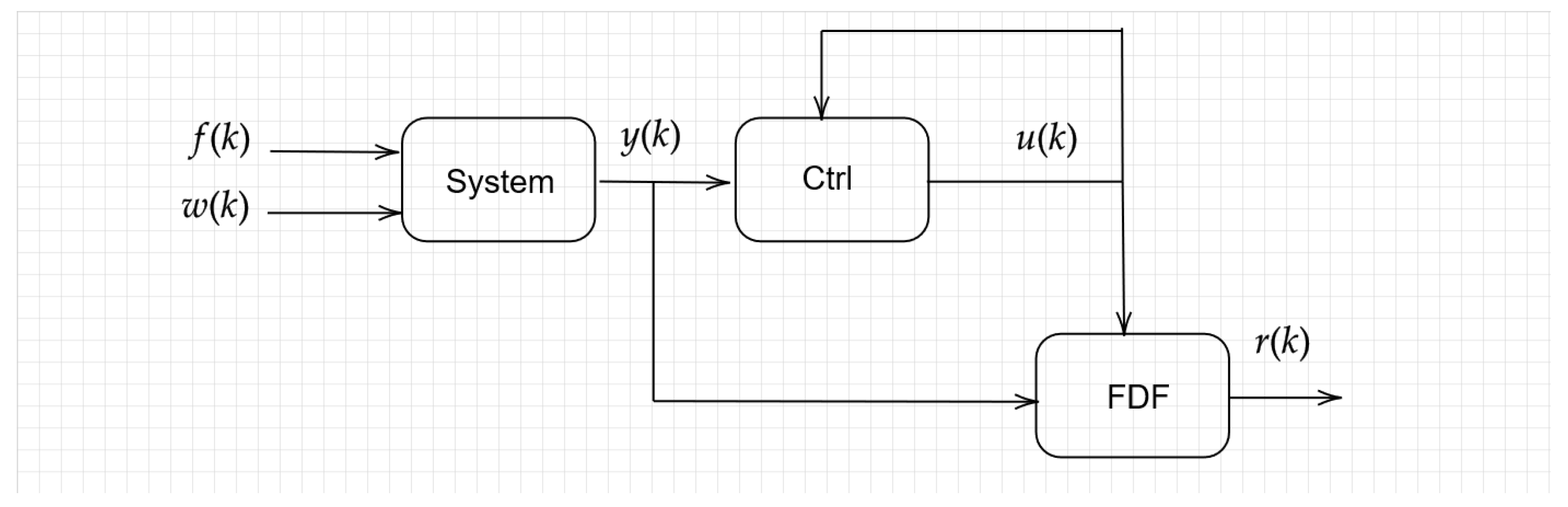
The block diagram of Figure 1 illustrates the FD scheme considered in this paper. Note that there are three elements composing the diagram: the system itself (${\mathcal{G}}_{{\theta }_k}$, which represents the plant subjected to a fault), the controller $K_{{\theta }_k}$, and the gain-scheduled FDF block ${\mathcal{F}}_{{\theta }_k}$.

The main purpose of this section is to design the FDF. Consider that the nonhomogeneous MJLS ${\mathcal{G}}_{{\theta }_k}$ is defined as

$${\mathcal{G}}_{{\theta }_k}\equiv \left\{\begin{array}{cc}\hfill x(k+1)& =A_{{\theta }_k}x\left(k\right)+B_{{\theta }_k}u\left(k\right)+J_{{\theta }_k}w\left(k\right)+F_{{\theta }_k}f\left(k\right)\hfill \\ \hfill y\left(k\right)& =C_{{\theta }_k}x\left(k\right)+D_{{\theta }_k}w\left(k\right)+E_{{\theta }_k}f\left(k\right)\hfill \end{array},\right.$$

(18)

where $x\left(k\right)\in {\mathbb{R}}^{n_x}$ denotes the system states vector, $u\left(k\right)\in {\mathbb{R}}^{n_u}$ represents the control input, $w\left(k\right)\in {\mathbb{R}}^{n_w}$ is the exogenous/noise input, $y\left(k\right)\in {\mathbb{R}}^{n_y}$ represents the measurement signals, and $f\left(k\right)\in {\mathbb{R}}^{n_f}$ is the fault signal that should be detected. We also assume that $w\left(k\right),f\left(k\right)\in {\mathcal{L}}^2$. Finally, when regarding the output-feedback control law, consider the following expression

$$\begin{array}{cc}\hfill & u\left(k\right)=K_{{\theta }_k}y\left(k\right).\hfill \end{array}$$

(19)

The controller ${\mathcal{K}}_{{\theta }_k}$ is assumed to be designed beforehand.

Remark 2. 

Although the formulation presented in this paper considers an output-feedback control law (19) that is mode-dependent (depends on ${\theta }_k$) but is parameter-independent (does not depend on ${\alpha }_k$ or the time-varying probabilities ${\rho }_{ij}\left(k\right)$), the synthesis of the FD filter presented next can be extended to deal with a parameter-dependent control law. Regardless of that, for both situations, it is imperative that the controller is designed a priori. The major implementation difference in the latter case is that the controller would be defined as gain-scheduled.

We define the gain-scheduled FDF under the aforementioned conditions as

$${\mathcal{F}}_{{\theta }_k}\equiv \left\{\begin{array}{cc}\hfill \eta (k+1)& ={\mathcal{A}}_{\eta {\theta }_k}\left(\alpha \left(k\right)\right)\eta \left(k\right)+{\mathcal{M}}_{\eta {\theta }_k}\left(\alpha \left(k\right)\right)u\left(k\right)+\cdots \hfill \\ & {\mathcal{B}}_{\eta {\theta }_k}\left(\alpha \left(k\right)\right)y\left(k\right)\hfill \\ \hfill r\left(k\right)& ={\mathcal{C}}_{\eta {\theta }_k}\left(\alpha \left(k\right)\right)\eta \left(k\right)\hfill \end{array},\right.$$

(20)

where $\eta \left(k\right)\in {\mathbb{R}}^{n_{\eta }}$ is the filter states, $r\left(k\right)\in {\mathbb{R}}^{n_r}$ is the residue signal, $u\left(k\right)$ is the control law given by (19), and $y\left(k\right)$ represents the measurement output. The FDF is scheduled in terms of the time-varying parameter $\alpha \left(k\right)$, which represents the variation in time of the MC. Consequently, it is assumed that the time-varying behavior of the MC is known or at least measurable. The purpose of the gain-scheduled FDF in (20) is to generate a residue signal $r\left(k\right)$, which is used to detect the fault.

Remark 3. 

All matrices that compose the filter (20) are written in the affine form as in (7), that is

$$\begin{array}{c}\hfill {\mathcal{A}}_{\eta i}\left({\beta }_k\right)={{\mathcal{A}}_{\eta i}}_{{\beta }_0}+\sum _{j=1}^m{\beta }_j\left(k\right){{\mathcal{A}}_{\eta i}}_{{\beta }_j},\end{array}$$

(21)

and similarly for ${\mathcal{M}}_{\eta i}\left({\beta }_k\right)$, ${\mathcal{B}}_{\eta i}\left({\beta }_k\right)$, ${\mathcal{C}}_{\eta i}\left({\beta }_k\right)$. Recall that the goal of this paper is to design the gain-scheduled FDF (20) where the schedule parameter represents the variation in the nonhomogeneous MC, as explained in Section 3.

We define $e\left(k\right)=r\left(k\right)-f\left(k\right)$ and the augmented system as

$${\mathcal{G}}_{aug}\equiv \left\{\begin{array}{c}\hfill \tilde{x}(k+1)={\tilde{A}}_{{\theta }_k}\left(\alpha \left(k\right)\right)\tilde{x}\left(k\right)+{\tilde{J}}_{{\theta }_k}\left(\alpha \left(k\right)\right)\tilde{w}\left(k\right)\\ \hfill e\left(k\right)={\tilde{C}}_{{\theta }_k}\left(\alpha \left(k\right)\right)\tilde{x}\left(k\right)+{\tilde{D}}_{{\theta }_k}\left(\alpha \left(k\right)\right)\tilde{w}\left(k\right)\end{array},\right.$$

(22)

where $\tilde{x}\left(k\right)=\left[x\left(k\right)\eta \left(k\right)\right]$, and $\tilde{w}\left(k\right)=\left[u\left(k\right)w\left(k\right)f\left(k\right)\right]$. The matrices that compose the augmented system are

$$\begin{array}{cc}\hfill & {\tilde{A}}_i\left(\alpha \left(k\right)\right)=\left[\begin{array}{cc}{A}_i& 0\\ {\mathcal{B}}_{\eta i}\left(\alpha \left(k\right)\right)C_i& {\mathcal{A}}_{\eta i}\left(\alpha \left(k\right)\right)\end{array}\right],\hfill \\ \hfill & {\tilde{J}}_i\left(\alpha \left(k\right)\right)=\left[\begin{array}{ccc}{B}_i& J_i& F_i\\ {\mathcal{M}}_{\eta i}\left(\alpha \left(k\right)\right)& {\mathcal{B}}_{\eta i}\left(\alpha \left(k\right)\right)D_i& {\mathcal{B}}_{\eta i}\left(\alpha \left(k\right)\right)E_i\end{array}\right],\mathrm{and}\hfill \\ \hfill & {\tilde{C}}_i\left(\alpha \left(k\right)\right)=\left[\begin{array}{cc}0& {\mathcal{C}}_{\eta i}\left(\alpha \left(k\right)\right)\end{array}\right],{\tilde{D}}_i\left(\alpha \left(k\right)\right)=\left[\begin{array}{ccc}0& 0& -I\end{array}\right].\hfill \end{array}$$

(23)

In order to provide an FDF (20), which generates a residue signal $r\left(k\right)$ that is robust against noise and associated with a fast response whenever a fault occurs, we set our goal as the synthesis of a proper FD filter by minimizing an upper bound $\gamma$ for the ${\mathcal{H}}_{\infty }$ norm of the augmented system (22), such that

$$\begin{array}{c}\hfill \underset{w\left(k\right)\in {\mathcal{L}}^2,{\parallel w\left(k\right)\parallel }_2\ne 0}{sup}\frac{{\parallel e\left(k\right)\parallel }_2}{{\parallel w\left(k\right)\parallel }_2}<\gamma .\end{array}$$

(24)

In the following, we present our main result of the paper, which provides parameter-dependent bilinear matrix inequalities (BMI) for the design of an FDF (20) for system (18) with ${\mathcal{H}}_{\infty }$ guaranteed cost. For compactness, hereafter, the dependence on time of parameter $\alpha \left(k\right)$ and $\alpha (k+1)$ is omitted, such that they will be respectively replaced by $\alpha$ and ${\alpha }^{+}$.

Theorem 1. 

If there exist, for all $i\in \mathbb{K}$, symmetric positive definite parameter-dependent matrices $Z_i\left(\alpha \right)$, $R_i\left(\alpha \right)$, ${\overline{Z}}_1\left({\alpha }^{+}\right)$, ${\overline{R}}_i\left({\alpha }^{+}\right)$, matrices $W_i\left(\alpha \right)$, ${\overline{W}}_i\left({\alpha }^{+}\right)$, $X_i\left(\alpha \right)$, $Y_i\left(\alpha \right)$${\mathcal{O}}_i\left(\alpha \right)$, ${\mathcal{B}}_{\eta i}\left(\alpha \right)$, ${\mathcal{M}}_{\eta i}\left(\alpha \right)$, ${\nabla }_i\left(\alpha \right)$ with appropriate dimensions, and a scalar $\xi \in (0,2)$, such that the BMIs (25) hold for all $\alpha ,{\alpha }^{+}\in {\mathrm{\Lambda }}_N$ and $i\in \mathbb{K}$,

$$\begin{array}{c}\left[\begin{array}{cccccccccc}{\Pi }_{11}& •& •& •& •& •& •& •& •& •\\ {\Pi }_{21}& {\Pi }_{22}& •& •& •& •& •& •& •& •\\ 0& 0& -{\gamma }^{2}I& •& •& •& •& •& •& •\\ 0& 0& 0& -{\gamma }^{2}I& •& •& •& •& •& •\\ 0& 0& 0& 0& -{\gamma }^{2}I& •& •& •& •& •\\ {\Pi }_{61}& {\Pi }_{62}& 0& 0& 0& {\Pi }_{66}& •& •& •& •\\ {\Pi }_{71}& {\Pi }_{72}& 0& 0& 0& {\Pi }_{76}& {\Pi }_{77}& •& •& •\\ {\Pi }_{81}& {\Pi }_{82}& {\mathrm{Y}}_i^a{\left(\alpha \right)}^{\prime }\left(B_i\right)& {\mathrm{Y}}_i^a{\left(\alpha \right)}^{\prime }\left(J_i\right)& {\mathrm{Y}}_i^a{\left(\alpha \right)}^{\prime }\left(F_i\right)& \xi {\Pi }_{81}& \xi {\Pi }_{82}& -\overline{Z}\left({\alpha }^{+}\right)& •& •\\ {\Pi }_{91}& {\Pi }_{92}& {\mathrm{Y}}_i^b{\left(\alpha \right)}^{\prime }{\mathcal{M}}_{\eta i}\left(\alpha \right)& {\Pi }_{94}& {\Pi }_{95}& \xi {\Pi }_{91}& \xi {\Pi }_{92}& -\overline{W}\left({\alpha }^{+}\right)& -\overline{R}\left({\alpha }^{+}\right)& •\\ {\nabla }_i\left(\alpha \right)& {\nabla }_i\left(\alpha \right)& 0& 0& -I& \xi {\nabla }_i\left(\alpha \right)& \xi {\nabla }_i\left(\alpha \right)& 0& 0& -I\end{array}\right]<0,\end{array}$$

(25)

where

$$\begin{array}{cc}\hfill & {\mathrm{Y}}_i^a\left(\alpha \right)=[{\rho }_{i1}^{1/2}\left(\alpha \right)I_{n_x}\cdots {\rho }_{i\sigma }^{1/2}\left(\alpha \right)I_{n_x}],{\mathrm{Y}}_i^b\left(\alpha \right)=[{\rho }_{i1}^{1/2}\left(\alpha \right)I_{n_{\eta }}\cdots {\rho }_{i\sigma }^{1/2}\left(\alpha \right)I_{n_{\eta }}],\hfill \\ \hfill & {\mathrm{Y}}_i^c\left(\alpha \right)=[{\rho }_{i1}^{1/2}\left(\alpha \right)I_{n_x+n_{\eta }}\cdots {\rho }_{i\sigma }^{1/2}\left(\alpha \right)I_{n_x+n_{\eta }}],{\Pi }_{11}=Z_i\left(\alpha \right)-\mathit{Her}\left(X_i\left(\alpha \right)\right),\hfill \\ \hfill & {\Pi }_{21}=W_i\left(\alpha \right)-Y_i\left(\alpha \right)-X_i{\left(\alpha \right)}^{\prime },{\Pi }_{61}=Z_i\left(\alpha \right)-\xi X_i{\left(\alpha \right)}^{\prime }-X_i\left(\alpha \right),\hfill \\ \hfill & {\Pi }_{71}=W_i\left(\alpha \right)-\xi X_i{\left(\alpha \right)}^{\prime }-Y_i\left(\alpha \right),{\Pi }_{81}={\mathrm{Y}}_i^a{\left(\alpha \right)}^{\prime }{A}_i{X}_i\left(\alpha \right),\hfill \\ & {\Pi }_{91}={\mathrm{Y}}_i^b{\left(\alpha \right)}^{\prime }({\mathcal{B}}_{\eta i}\left(\alpha \right)C_i{X}_i\left(\alpha \right)+{\mathcal{O}}_i\left(\alpha \right)),{\Pi }_{22}=R_i\left(\alpha \right)-\mathit{Her}\left(Y_i\left(\alpha \right)\right),\hfill \\ \hfill & {\Pi }_{62}=W_i{\left(\alpha \right)}^{\prime }-\xi Y_i{\left(\alpha \right)}^{\prime }-X_i\left(\alpha \right),{\Pi }_{72}=R_i\left(\alpha \right)-\xi Y_i{\left(\alpha \right)}^{\prime }-Y_i\left(\alpha \right),\hfill \\ \hfill & {\Pi }_{82}={\Pi }_{81},{\Pi }_{92}={\Pi }_{91},{\Pi }_{94}={\mathrm{Y}}_i^b{\left(\alpha \right)}^{\prime }{\mathcal{B}}_{\eta i}\left(\alpha \right)D_i,\hfill \\ \hfill & {\Pi }_{95}={\mathrm{Y}}_i^b{\left(\alpha \right)}^{\prime }\left({\mathcal{B}}_{\eta i}\left(\alpha \right)E_i\right),{\Pi }_{66}=-\xi \mathit{Her}\left(X_i\left(\alpha \right)\right),\hfill \\ & {\Pi }_{76}=-\xi (Y_i\left(\alpha \right)-X_i{\left(\alpha \right)}^{\prime }),{\Pi }_{77}=-\xi \mathit{Her}\left(Y_i\left(\alpha \right)\right),\hfill \end{array}$$

and

$$\begin{array}{cc}\hfill \overline{Z}\left({\alpha }^{+}\right)=\mathrm{diag}({\overline{Z}}_1\left({\alpha }^{+}\right),\dots ,{\overline{Z}}_{\sigma }\left({\alpha }^{+}\right)),& {\overline{W}}^{+}\left({\alpha }^{+}\right)=\mathrm{diag}({\overline{W}}_1^{+}\left({\alpha }^{+}\right),\dots ,{\overline{W}}_{\sigma }\left({\alpha }^{+}\right)),\hfill \\ \hfill {\overline{R}}_i\left({\alpha }^{+}\right)=& \mathrm{diag}({\overline{R}}_1\left({\alpha }^{+}\right),\dots ,{\overline{R}}_{\sigma }\left({\alpha }^{+}\right)),\hfill \end{array}$$

(26)

then γ is an upper bound for the ${\mathcal{H}}_{\infty }$ norm of the augmented system (22), where the matrices that compose the FDF in the form of (20) are given by ${\mathcal{A}}_{\eta i}\left(\alpha \right)={\mathcal{O}}_i\left(\alpha \right)Y_i{\left(\alpha \right)}^{-1}$, ${\mathcal{B}}_{\eta i}\left(\alpha \right)$, ${\mathcal{M}}_{\eta i}\left(\alpha \right)$, ${\mathcal{C}}_{\eta i}\left(\alpha \right)={\nabla }_i{Y}_i{\left(\alpha \right)}^{-1}\left(\alpha \right)$ for all $i\in \mathbb{K}$.

Proof of Theorem 1. 

Consider the augmented matrices as from (23), and define the matrices $P_i\left(\alpha \right)$ and $H_i\left(\alpha \right)$ according to

$$\begin{array}{c}\hfill P_i\left(\alpha \right)=\left[\begin{array}{cc}{Z}_i\left(\alpha \right)& •\\ W_i\left(\alpha \right)& R_i\left(\alpha \right)\end{array}\right],H_i\left(\alpha \right)=\left[\begin{array}{cc}{X}_i\left(\alpha \right)& X_i\left(\alpha \right)\\ Y_i\left(\alpha \right)& Y_i\left(\alpha \right)\end{array}\right].\end{array}$$

(27)

In addition, we define the matrices ${\overline{P}}_i\left({\alpha }^{+}\right)$ and $\overline{P}\left({\alpha }^{+}\right)$ as follows:

$$\begin{array}{c}\hfill {\overline{P}}_i\left({\alpha }^{+}\right)=\left[\begin{array}{cc}{\overline{Z}}_i\left({\alpha }^{+}\right)& •\\ {\overline{W}}_i\left({\alpha }^{+}\right)& {\overline{R}}_i\left({\alpha }^{+}\right)\end{array}\right],\overline{P}\left({\alpha }^{+}\right)=\mathrm{diag}({\overline{P}}_i\left({\alpha }^{+}\right),\dots ,{\overline{P}}_{\sigma }\left({\alpha }^{+}\right)).\end{array}$$

(28)

Consider the following change of variables: ${\mathcal{O}}_i\left(\alpha \right)={\mathcal{A}}_{\eta i}\left(\alpha \right)Y_i\left(\alpha \right)$, ${\nabla }_i\left(\alpha \right)={\mathcal{C}}_{\eta i}\left(\alpha \right)Y_i\left(\alpha \right)$. Then we obtain the following identities:

$$\begin{array}{c}\hfill \begin{array}{cc}{\tilde{A}}_i\left(\alpha \right)H_i\left(\alpha \right)\hfill & =\left[\begin{array}{cc}{A}_i+B_i{K}_i\left(\alpha \right)C_i& 0\\ {\mathcal{M}}_{\eta i}\left(\alpha \right)K_i\left(\alpha \right)C_i+{\mathcal{B}}_{\eta i}\left(\alpha \right)C_i& {\mathcal{A}}_{\eta i}\left(\alpha \right)\end{array}\right]\left[\begin{array}{cc}{X}_i\left(\alpha \right)& X_i\left(\alpha \right)\\ Y_i\left(\alpha \right)& Y_i\left(\alpha \right)\end{array}\right]\hfill \\ \hfill & =\left[\begin{array}{cc}(A_i+B_i{K}_i\left(\alpha \right)C_i)X_i\left(\alpha \right)& (A_i+B_i{K}_i\left(\alpha \right)C_i)X_i\left(\alpha \right)\\ {\Xi }_i\left(\alpha \right)+{\mathcal{A}}_{\eta i}\left(\alpha \right)Y_i\left(\alpha \right)& {\Xi }_i\left(\alpha \right)+{\mathcal{A}}_{\eta i}\left(\alpha \right)Y_i\left(\alpha \right)\end{array}\right],\hfill \\ {\tilde{C}}_i\left(\alpha \right)H_i\left(\alpha \right)\hfill & =\left[\begin{array}{cc}0& {\mathcal{C}}_{\eta i}\left(\alpha \right)\end{array}\right]\left[\begin{array}{cc}{X}_i\left(\alpha \right)& X_i\left(\alpha \right)\\ Y_i\left(\alpha \right)& Y_i\left(\alpha \right)\end{array}\right]\hfill \\ \hfill & =\left[\begin{array}{cc}{\mathcal{C}}_{\eta i}\left(\alpha \right)Y_i\left(\alpha \right)& {\mathcal{C}}_{\eta i}\left(\alpha \right)Y_i\left(\alpha \right)\end{array}\right],\hfill \end{array}\end{array}$$

(29)

where ${\Xi }_i\left(\alpha \right)=({\mathcal{M}}_{\eta i}\left(\alpha \right)K_i{C}_i+{\mathcal{B}}_{\eta i}\left(\alpha \right)C_i)X_i\left(\alpha \right).$ Consequently, the BMI (25) can be rewritten as

$$\begin{array}{c}\hfill \left[\begin{array}{ccccc}{P}_i\left(\alpha \right)-\mathrm{Her}\left(H_i\left(\alpha \right)\right)& •& •& •& •\\ 0& -{\gamma }^{2}I& •& •& •\\ P_i\left(\alpha \right)-\xi H_i{\left(\alpha \right)}^{\prime }-H_i\left(\alpha \right)& 0& -\xi \mathrm{Her}\left(H_i\left(\alpha \right)\right)& •& •\\ {\mathrm{Y}}_i^c{\left(\alpha \right)}^{\prime }{\tilde{A}}_i\left(\alpha \right)H_i\left(\alpha \right)& {\mathrm{Y}}_i^c{\left(\alpha \right)}^{\prime }{\tilde{J}}_i\left(\alpha \right)& \xi {\mathrm{Y}}_i^c{\left(\alpha \right)}^{\prime }{\tilde{A}}_i\left(\alpha \right)H_i\left(\alpha \right)& -\overline{P}\left({\alpha }^{+}\right)& •\\ {\tilde{C}}_i\left(\alpha \right)H_i\left(\alpha \right)& {\tilde{D}}_i\left(\alpha \right)& \xi {\tilde{C}}_i\left(\alpha \right)H_i\left(\alpha \right)& 0& -I\end{array}\right]<0.\end{array}$$

(30)

By using the projection lemma (see [24]), (30) can be rewritten as follows,

$$\begin{array}{c}\hfill \mathcal{D}+{\mathcal{U}}^{\prime }{H}_i\mathcal{V}+\mathcal{V}{H}_i^{\prime }\mathcal{U}<0,\end{array}$$

(31)

where

$$\begin{array}{c}\hfill \mathcal{D}=\left[\begin{array}{ccccc}{P}_i& •& •& •& •\\ 0& -{\gamma }^{2}I& •& •& •\\ P_i& 0& 0& •& •\\ 0& {{\mathrm{Y}}_i^c}^{\prime }{\tilde{J}}_i& 0& -{\overline{P}}^{+}& •\\ 0& {\tilde{D}}_i& 0& 0& -I\end{array}\right],{\mathcal{U}}^{\prime }=\left[\begin{array}{c}-I\\ 0\\ -I\\ {{\mathrm{Y}}_i^c}^{\prime }{\tilde{A}}_i\\ {\tilde{C}}_i\end{array}\right],{\mathcal{V}}^{\prime }=\left[\begin{array}{c}I\\ 0\\ \xi I\\ 0\\ 0\end{array}\right].\end{array}$$

(32)

(Observe that in the remaining of the proof, the time-varying parameter $\alpha$ is omitted for notation simplicity, as well as the dependence on ${\alpha }^{+}$, which will be replaced by the superscript index “+”.)

By taking the following basis for the null space of $\mathcal{U}$ and $\mathcal{V}$

$$\begin{array}{c}\hfill {\mathcal{N}}_{\mathcal{U}}=\left[\begin{array}{cccc}I& 0& 0& 0\\ 0& I& 0& 0\\ -I& 0& {\tilde{A}}_i^{\prime }{\mathrm{Y}}_i^c& {\tilde{C}}_i^{\prime }\\ 0& 0& I& 0\\ 0& 0& 0& I\end{array}\right],{\mathcal{N}}_{\mathcal{V}}=\left[\begin{array}{cccc}\xi I& 0& 0& 0\\ 0& I& 0& 0\\ -I& 0& 0& 0\\ 0& 0& I& 0\\ 0& 0& 0& I\end{array}\right]\end{array}$$

(33)

and by applying the equivalence conditions of the projection lemma, we get

$$\begin{array}{c}\hfill N_{\mathcal{U}}^{\prime }\mathcal{D}{N}_{\mathcal{U}}=\left[\begin{array}{cccc}-P_i& •& •& •\\ 0& -{\gamma }^{2}I& •& •\\ {{\mathrm{Y}}_i^c}^{\prime }{\tilde{A}}_i{P}_i& {{\mathrm{Y}}_i^c}^{\prime }{\tilde{J}}_i^{\prime }& -{\overline{P}}^{+}& •\\ {\tilde{C}}_i{P}_i& {\tilde{D}}_i& 0& -I\end{array}\right]<0,\end{array}$$

(34)

$$\begin{array}{c}\hfill N_{\mathcal{V}}^{\prime }\mathcal{D}{N}_{\mathcal{V}}=\left[\begin{array}{cccc}({\xi }^2-2\xi )P_i& •& •& •\\ 0& -{\gamma }^{2}I& •& •\\ 0& {{\mathrm{Y}}_i^c}^{\prime }{\tilde{J}}_i& -{\overline{P}}^{+}& •\\ 0& {\tilde{D}}_i& 0& -I\end{array}\right]<0.\end{array}$$

(35)

Notice that from the first term in (35) we can state that $0<\xi <2$. Now, pre- and postmultiplying (34) by $\mathrm{diag}(X_i,I,{\overline{\mathcal{X}}}^{+},I)$, where $X_i=P_i^{-1}$, ${\overline{\mathcal{X}}}^{+}={\left({\overline{P}}^{+}\right)}^{-1}$, we obtain

$$\begin{array}{c}\hfill \left[\begin{array}{cccc}-X_i& •& •& •\\ 0& -{\gamma }^{2}I& •& •\\ {\overline{\mathcal{X}}}^{+}{{\mathrm{Y}}_i^c}^{\prime }{\tilde{A}}_i& {\overline{\mathcal{X}}}^{+}{{\mathrm{Y}}_i^c}^{\prime }{\tilde{J}}_i& -{\overline{\mathcal{X}}}^{+}& •\\ {\tilde{C}}_i& {\tilde{D}}_i& 0& -I\end{array}\right]<0.\end{array}$$

(36)

Notice that ${\widehat{\mathcal{X}}}^{+}$ represents a block diagonal matrix given by

$$\begin{array}{c}\hfill {\widehat{\mathcal{X}}}^{+}=\mathrm{diag}({\overline{X}}_1^{+},\cdots ,{\overline{X}}_{\sigma }^{+}),\end{array}$$

(37)

with ${\overline{X}}_i^{+}={\left({\overline{P}}_i^{+}\right)}^{-1}$. By using the Schur complement in (36) and noticing that

$$\begin{array}{c}\hfill {\mathrm{Y}}_i^c{\overline{\mathcal{X}}}^{+}{{\mathrm{Y}}_i^c}^{\prime }=\sum _{j=1}^{\sigma }{\rho }_{ij}{\overline{X}}_j^{+},\end{array}$$

(38)

we have the condition (15) satisfied, so that the result follows from the bounded real lemma, presented in Lemma 1, for the nonhomogenous MJLS.    □

Remark 4. 

Observe that the conditions of Theorem 1 constitute of infinite-dimensional problems, which can be solved by using homogeneous polynomial approximations for the optimization variables (LMI relaxations) and then testing the positivity of the polynomial matrix inequalities by means of a finite set of LMIs. For this purpose, the authors strongly recommend the use of the toolbox robust LMI parser (ROLMIP), whose tutorial can be found in [25].

Remark 5. 

Theorem 1 can be adapted to handle the FDF synthesis problem for homogeneous MJLS with constant or uncertain but time-invariant probability matrix by simply making $\alpha (k+1)=\alpha \left(k\right)=\alpha$.

The constraints presented in Theorem 1 are BMIs, which means that is necessary to use appropriate tools in order to solve them. Among a number of techniques available in the literature [26,27,28], we employ the coordinate descend algorithm (CDA), since it is a well-known and widely used tool to solve such issues. Accordingly, an iterative procedure based in CDA is given below to solve Theorem 1.

In Algorithm 1, $\varphi$ represents the stop criteria and $t_{\max }$ is the maximum number of iterations allowed. Observe that if a solution is found in the first iteration of CDA, the iterative procedure will converge to an optimized solution or at least keep the same solution found in the first iteration. The CDA is better detailed in [26,27].

Algorithm 1 Coordinate descent algorithm.

Coordinate descent algorithm (CDA): Input:${\mathcal{B}}_{\eta i}$, $\gamma$, $t_{\max }$, $\varphi$. Output:${\mathcal{A}}_{\eta i}$, ${\mathcal{B}}_{\eta i}$, ${\mathcal{M}}_{\eta i}$, ${\mathcal{C}}_{\eta i}$. Initialization: While:$\frac{{\gamma }^{t-1}-{\gamma }^t}{{\gamma }^{t-1}}\le \eta$ or $t\le t_{\max }$ do: Step 1: Find a solution for the LMI constraint (25) obtaining the values of X using as an input ${\mathcal{B}}_i$, which can be obtained by using any method, for example, the one in Theorem 1 in [7]. Step 2: Now find a solution for the same LMI constraint (25) to obtain ${\mathcal{A}}_{\eta i}$, ${\mathcal{B}}_{\eta i}$, ${\mathcal{M}}_{\eta i}$, ${\mathcal{C}}_{\eta i}$, but this time by using X as an input. Also obtain the value of $\gamma$.

6. Numerical Example

To illustrate the applicability of the theoretical results, a numerical example of a coupled tanks model (see Figure 2) is presented next. In this example, we assume that the plant itself is time-invariant, nevertheless, there are some time-varying parameters associated with the model of the communication network, which is represented by a nonhomogeneous Markov chain.

6.1. Simulation Setup

The parameters and modeling of the coupled tanks system were extracted from [29], such that the continuous-time state-space matrices are given by

$$\begin{array}{c}A=\left[\begin{array}{cc}-0.0239& -0.0127\\ 0.0127& -0.0285\end{array}\right],B=\left[\begin{array}{c}0.71\\ 0\end{array}\right],\\ J=\left[\begin{array}{c}0.0071\\ 0\end{array}\right],F=\left[\begin{array}{c}0.071\\ 0\end{array}\right],K=\left[\begin{array}{cc}-1.03& -0.33\end{array}\right].\end{array}$$

(39)

The sampling time used is $T_s=1$s. Note that in order to represent the fault as an abnormal input on the first tank, the matrix associated with the fault signal F is $10\%$ of the control input matrix B.

Regarding the network modeling, we assume that each tank is far away from the other; therefore, data gathered from each sensor is transmitted via two distinct networks. Network 1 transmits the measurement of the first tank, and Network 2 transmits the measurements of the second tank. The transmission of the measurement signals through a semireliable communication network is modeled by using a simplified Gilbert–Elliot model, as done in [30] while the packet dropout is represented by the zero-input approach from [31], meaning that when a packet loss occurs, we assume that the value of the received signal is null. Hence, the complete network behavior is represented by four distinct operation modes, as illustrated by Figure 3. The first one is that where all the measurements are correctly transmitted (called “Ok Ok” in Figure 3); the second one considers that the measurement on the first tank is successfully transmitted, but occurs a packet dropout of the measurement from the second tank (called “Ok Drop” in Figure 3); the third case is the opposite of the second one (called “Drop Ok” in Figure 3); and the last mode represents the case where all measurements were lost (called “Drop Drop” in Figure 3).

Remark 6. 

It is essential to point out that the proposed solution allows modeling the network packet dropout rate varying in time. However, the feasibility of the proposed solution is dictated by three main features, the system dynamic, the number of Markov modes, and range variation. Therefore, it is important to keep in mind that an overly complex Markov chain with a high range of variation will request more computational effort, and in some situations, a feasible solution may not be achieved.

From the previous network description, we can write the matrices that represent the measurement signal $y\left(k\right)$ are denoted by (the subindex is associated with the network operation mode)

$$\begin{array}{c}\hfill \begin{array}{c}{C}_1=\left[\begin{array}{cc}1& 0\\ 0& 1\end{array}\right],C_2=\left[\begin{array}{cc}1& 0\\ 0& 0\end{array}\right],C_3=\left[\begin{array}{cc}0& 0\\ 0& 1\end{array}\right],C_4=\left[\begin{array}{cc}0& 0\\ 0& 0\end{array}\right],\\ D_1=\left[\begin{array}{c}0.01\\ 0.01\end{array}\right],D_2=\left[\begin{array}{c}0.01\\ 0\end{array}\right],D_3=\left[\begin{array}{c}0\\ 0.01\end{array}\right],D_4=\left[\begin{array}{c}0\\ 0\end{array}\right],\\ E_{1,2,3,4}=\left[\begin{array}{c}0\\ 0\end{array}\right]\end{array}\end{array}.$$

(40)

Observe that we imposed E equal to zero in all modes because despite the fault in the example representing an abnormal input on the first tank, the sensors are assumed to be healthy throughout the simulation.

To illustrate the flexibility of the proposed approach, a particular scenario was tested. Assume that we solely know the boundary of the transition probability matrix that governs the jumps among the four network modes. Another important assumption considered in the design process is that in the fourth mode, Drop Drop, where there is no sensor information, the scheduling parameter is not accessible, implying that the matrices that compose the FDF for this mode are designed in the robust form instead of the affine form.

The time-varying transition probability matrix is given by

$$\begin{array}{cc}\hfill & \mathbb{P}\left(k\right)=\underset{{\mathbb{P}}_{{\beta }_0}}{\underbrace{\left[\begin{array}{cccc}0.3& 0.2& 0.1& 0.4\\ 0.1& 0.4& 0.3& 0.2\\ 0.1& 0.2& 0.4& 0.3\\ 0.1& 0.2& 0.1& 0.6\end{array}\right]}}+\underset{{\mathbb{P}}_{{\beta }_1}\left(k\right)}{\underbrace{\left[\begin{array}{cccc}0& 0& 0& 0\\ 1& -1& 0& 0\\ 0& 0& 0& 0\\ 0& 0& 0& 0\end{array}\right]{\beta }_1\left(k\right)}}+\underset{{\mathbb{P}}_{{\beta }_2}\left(k\right)}{\underbrace{\left[\begin{array}{cccc}0& 0& 0& 0\\ 0& 0& 0& 0\\ 0& 1& -1& 0\\ 0& 0& 0& 0\end{array}\right]{\beta }_2\left(k\right)}},\hfill \end{array}$$

(41)

where ${\beta }_1\left(k\right)\in [0,0.3]$, ${\beta }_2\left(k\right)\in [0,0.3]$, and by consequence ${\beta }_r\left(k\right)=0{\alpha }_{r1}\left(k\right)+0.3{\alpha }_{r2}\left(k\right),r=1,2$, where $\alpha \left(k\right)\in {\mathrm{\Lambda }}_N={\mathrm{\Lambda }}_2\times {\mathrm{\Lambda }}_2$, $N=(2,2)$.

Additionally, the transition probability among network states represented in Figure 3 by ${\rho }_{ij}\left(k\right)$ corresponds to an entry in the transition probability matrix $\mathbb{P}\left(k\right)$. Those transition probabilities depend on time as follows,

$${\rho }_{ij}\left(k\right)=\rho 0_{ij}+{\beta }_1\left(k\right)\rho 1_{ij}+{\beta }_2\left(k\right)\rho 2_{ij},$$

where $\rho 0_{ij}$, $\rho 1_{ij}$ and $\rho 2_{ij}$ represent the elements of ith row and jth column from the following matrices ${\mathbb{P}}_{{\beta }_0}\left(k\right)$, ${\mathbb{P}}_{{\beta }_1}\left(k\right)$ and ${\mathbb{P}}_{{\beta }_2}\left(k\right)$ of Equation (41). Furthermore, the time evolution of the time-varying parameters ${\beta }_1\left(k\right)$ and ${\beta }_2\left(k\right)$ is illustrated by Figure 4.

By using the above numerical values of the plant and the network, we are now able to apply Theorem 1 to provide a solution for the FDF, so that the filter matrices in (20) (with $\xi =0.9$ in Theorem 1) are given by

$$\begin{array}{c}\hfill \begin{array}{cc}\hfill & {\mathcal{A}}_{\eta 1_{\beta 0}}=\left[\begin{array}{cc}0.56& 0.00\\ -0.00& -0.00\end{array}\right],{\mathcal{A}}_{\eta 1_{\beta 1}}=\left[\begin{array}{cc}-0.01& -0.00\\ 0.00& -0.00\end{array}\right],{\mathcal{A}}_{\eta 1_{\beta 2}}=\left[\begin{array}{cc}-0.01& -0.00\\ 0.00& -0.00\end{array}\right],\hfill \\ \hfill & {\mathcal{A}}_{\eta 2_{\beta 0}}=\left[\begin{array}{cc}0.12& 0.00\\ 0.00& 0.00\end{array}\right],{\mathcal{A}}_{\eta 2_{\beta 1}}=\left[\begin{array}{cc}-0.01& -0.00\\ -0.00& -0.00\end{array}\right],{\mathcal{A}}_{\eta 2_{\beta 2}}=\left[\begin{array}{cc}-0.01& -0.00\\ -0.00& -0.00\end{array}\right],\hfill \\ \hfill & {\mathcal{A}}_{\eta 3_{\beta 0}}=\left[\begin{array}{cc}0.00& -0.02\\ -0.00& -0.00\end{array}\right],{\mathcal{A}}_{\eta 3_{\beta 1}}=\left[\begin{array}{cc}-0.00& 0.03\\ 0.00& 0.00\end{array}\right],{\mathcal{A}}_{\eta 3_{\beta 2}}=\left[\begin{array}{cc}-0.00& 0.03\\ 0.00& 0.00\end{array}\right]\hfill \\ \hfill & {\mathcal{A}}_{\eta 4_{\beta 0}}=\left[\begin{array}{cc}-0.00& -0.00\\ 0.00& -0.00\end{array}\right],\hfill \\ \hfill & {\mathcal{B}}_{\eta 1_{\beta 0}}=\left[\begin{array}{cc}0.04& 0.00\\ -0.00& 0.00\end{array}\right],{\mathcal{B}}_{\eta 1_{\beta 1}}=\left[\begin{array}{cc}0.01& -0.00\\ -0.00& 0.00\end{array}\right],{\mathcal{B}}_{\eta 1_{\beta 2}}=\left[\begin{array}{cc}0.01& -0.00\\ -0.00& 0.00\end{array}\right],\hfill \\ \hfill & {\mathcal{B}}_{\eta 2_{\beta 0}}=\left[\begin{array}{cc}0.03& 0.00\\ 0.00& 0.00\end{array}\right],{\mathcal{B}}_{\eta 2_{\beta 1}}=\left[\begin{array}{cc}0.01& 0.00\\ 0.00& 0.00\end{array}\right],{\mathcal{B}}_{\eta 2_{\beta 2}}=\left[\begin{array}{cc}0.01& 0.00\\ 0.00& 0.00\end{array}\right],\hfill \\ \hfill & {\mathcal{B}}_{\eta 3_{\beta 0}}=\left[\begin{array}{cc}0.00& 0.03\\ 0.00& 0.00\end{array}\right],{\mathcal{B}}_{\eta 3_{\beta 1}}=\left[\begin{array}{cc}0& 0.01\\ 0& 0.00\end{array}\right],{\mathcal{B}}_{\eta 3_{\beta 2}}=\left[\begin{array}{cc}0& 0.01\\ 0& 0.00\end{array}\right],\hfill \\ \hfill & {\mathcal{B}}_{\eta 4_{\beta 0}}=\left[\begin{array}{cc}0.00& 0.00\\ 0.00& 0.00\end{array}\right],\hfill \\ \hfill & {\mathcal{M}}_{\eta 1_{\beta 0}}=\left[\begin{array}{c}0.04\\ 0.00\end{array}\right],{\mathcal{M}}_{\eta 1_{\beta 1}}=\left[\begin{array}{c}0.01\\ 0.00\end{array}\right],{\mathcal{M}}_{\eta 1_{\beta 2}}=\left[\begin{array}{c}0.01\\ 0.00\end{array}\right],\hfill \\ \hfill & {\mathcal{M}}_{\eta 2_{\beta 0}}=\left[\begin{array}{c}0.03\\ 0.00\end{array}\right],{\mathcal{M}}_{\eta 2_{\beta 1}}=\left[\begin{array}{c}0.01\\ 0.00\end{array}\right],{\mathcal{M}}_{\eta 2_{\beta 2}}=\left[\begin{array}{c}0.01\\ 0.00\end{array}\right],\hfill \\ \hfill & {\mathcal{M}}_{\eta 3_{\beta 0}}=\left[\begin{array}{c}0.03\\ 0.00\end{array}\right],{\mathcal{M}}_{\eta 3_{\beta 1}}=\left[\begin{array}{c}0.01\\ 0.00\end{array}\right],{\mathcal{M}}_{\eta 3_{\beta 2}}=\left[\begin{array}{c}0.01\\ 0.00\end{array}\right],\hfill \\ \hfill & {\mathcal{M}}_{\eta 4_{\beta 0}}=\left[\begin{array}{c}0.01\\ 0.00\end{array}\right],\hfill \\ \hfill & {\mathcal{C}}_{\eta 1_{\beta 0}}=\left[\begin{array}{cc}1.20& -0.12\end{array}\right],{\mathcal{C}}_{\eta 1_{\beta 1}}=\left[\begin{array}{cc}-0.01& -0.01\end{array}\right],{\mathcal{C}}_{\eta 1_{\beta 2}}=\left[\begin{array}{cc}-0.01& -0.01\end{array}\right],\hfill \\ \hfill & {\mathcal{C}}_{\eta 2_{\beta 0}}=\left[\begin{array}{cc}0.32& 0.01\end{array}\right],{\mathcal{C}}_{\eta 2_{\beta 1}}=\left[\begin{array}{cc}-0.00& -0.00\end{array}\right],{\mathcal{C}}_{\eta 2_{\beta 2}}=\left[\begin{array}{cc}-0.01& -0.00\end{array}\right],\hfill \\ \hfill & {\mathcal{C}}_{\eta 3_{\beta 0}}=\left[\begin{array}{cc}0.02& -0.02\end{array}\right],{\mathcal{C}}_{\eta 3_{\beta 1}}=\left[\begin{array}{cc}-0.00& 0.01\end{array}\right],{\mathcal{C}}_{\eta 3_{\beta 2}}=\left[\begin{array}{cc}-0.00& 0.01\end{array}\right],\hfill \\ \hfill & {\mathcal{C}}_{\eta 4_{\beta 0}}=\left[\begin{array}{cc}-0.01& -0.00\end{array}\right].\hfill \end{array}\end{array}$$

(42)

6.2. Simulation Result

In this section, for comparison purposes, we present simulation results with one design of FDF that assumes complete knowledge of the modes and the other design that uses the results from [8], where an ${\mathcal{H}}_{\infty }$ guaranteed cost is used as the performance criterion. This comparison is important to show that the consideration of the nonhomogeneous MC impacts the FDF performance. This particular paper was chosen to be compared with the proposed approach since both are based on the MJLS framework and are based on the $H_{\infty }$ norm. Another critical piece of information that can be gathered from this comparison is the complexity of the problem versus performance gain. We remind that the parameters ${\beta }_1\left(k\right)$, ${\beta }_2\left(k\right)$ are assumed to be instantly measurable. Hence, the parameters ${\beta }_1\left(k\right)$, ${\beta }_2\left(k\right)$ vary during the simulation according to the information provided by Figure 4.

There are three faults that the system is subjected to during simulation. Those faults, presented in Figure 5, were applied on the first tank, and both affect the signal multiplying matrix F in (39). A Monte Carlo simulation with 100 interactions was performed, and Figure 6 and Figure 7 illustrate the obtained results.

Figure 6 presents the system’s states when subjected to all three fault cases, and also a case without fault. From Figure 6, it is possible to observe that the faults do not surpass $10\%$ of the nominal state value.

The residue signal generated by the FDFs for each type of fault, and also the case without fault are presented in Figure 7. We may state that all the FDF worked as expected, have been affected by the faults when it occurs, and that when there is not a fault the residue kept close to zero. Note that the results obtained by the FDF designed with the complete knowledge of the modes show more sensitivity against the fault, which helps to detect the fault faster.

A fault-detection procedure has two major stages: the residue generation and evaluation process. In Figure 7, the residue signals obtained via simulation were presented. To execute the next stage, it is necessary to define two tools: the evaluation function ($\mathrm{EVAL}\left(k\right)$) and the threshold (TH). The definition of these two tools are a deep issue that will not be tackled here; therefore, for a more detailed discussion, please refer to [1,4]. Consider the following definition for the evaluation function:

$$\begin{array}{c}\hfill \mathrm{EVAL}\left(k\right)\triangleq \sqrt{\sum _{i=k-L}^{k}r{\left(i\right)}^{\prime }r\left(i\right)},\end{array}$$

(43)

where L represents the evaluation window, which, in this particular simulation is assumed to be $L=250$. The threshold TH is used to assess the evaluation function $\mathrm{EVAL}\left(k\right)$. If $\mathrm{EVAL}\left(k\right)>\mathrm{TH}$ there is a fault, and for the opposite case there is no fault. For the simulations, the value of the threshold was arbitrarily set to $\mathrm{TH}=5$. From the aforementioned, the evaluation functions for all the FDF considering each fault were calculated and presented in Figure 8.

As can be seen in Figure 8, all FDFs are able to detect the different faults; however, there is a clear difference in the time that it takes for each FDF, as indicated by

Table 1. The detection window for all FDF considering each fault after the Monte Carlo simulation.

Design Method	Fault 1 (k)	Fault 2 (k)	Fault 3 (k)
Theorem 1 (All)	$\left[105114\right]$	$\left[133140\right]$	$\left[183188\right]$
[8]	$\left[112117\right]$	$\left[145156\right]$	$\left[202212\right]$

. Note that the proposed approach presented a faster detection for all three faults. This occurred because the proposed solution considers a more trustworthy model. Thus, an abnormal change can be detected more quickly.

Another interesting aspect is that the FDF designed by using [8] (the FDF under the assumption that the MC is homogeneous) is affected by the variation even when there is no fault occurrence. This particularity can be observed in Figure 8h, where the evaluation value drifts away from zero. This is an issue that affects the performance of the FDF, since it may cause false alarms. Note that this phenomenon does not occur on the FDF designed by using the proposed approach, showing that the consideration of the nonhomogeneous MC is useful to increase the performance of the FDF, especially for the situation where a nonhomogeneous MC is used to model characteristics that are inherently time-varying, such as a wireless sensor network. The last piece of information gathered from the simulation is that even though the proposed solution was based on more assumptions and a higher number of LMI constraints, which is clearly more computationally costly compared to the results in [8], the proposed approach provides superior performance.

7. Conclusions

The main contribution of this paper is the development of a new design method for gain-scheduled FDF considering that the plant measurement signals are transmitted through a network whose dropouts are modeled by using the MJLS theory, with the Markov chain being nonhomogeneous. The premise of nonhomogeneous MC is tackled by using the LPV modelling, specifically applied to the probability transition matrix, allowing us to design the FDF under this particular circumstance. The FDF synthesis results are obtained by using parameter-dependent LMI constraints that employ ${\mathcal{H}}_{\infty }$ norm as performance index. Since the gain-scheduled FDF varies according to the probability transition matrix variation, the proposed FDF is optimal for all the variation range of the Markov chain. To illustrate this, a comparison between the proposed technique with another method from the literature that does not contemplate the nonhomogeneous MC assumption was made. The simulation results show that the nonhomogeneous assumption positively impacts the FDF performance, allowing the proposed technique to detect the fault in a smaller time window, which can be seen in Table 1. Furthermore the FDF does not present false variations in the evaluation function, that could be identified as faults, when a fault does not occur, as can be seen in Figure 8g,h. A possible next step along this research line would be to include a sensitivity ${\mathcal{H}}_{-}$ index in the design to further improve the FDF performance.

References

1. Chen, J.; Patton, R.J. Robust Model-Based Fault Diagnosis for Dynamic Systems; Springer Science & Business Media: Berlin/Heidelberg, Germany, 2012; Volume 3. [Google Scholar]
2. Patton, R.J.; Frank, P.M.; Clark, R.N. Issues of Fault Diagnosis for Dynamic Systems; Springer Science & Business Media: Berlin/Heidelberg, Germany, 2013. [Google Scholar]
3. Isermann, R.; Schwarz, R.; Stolzl, S. Fault-tolerant drive-by-wire systems. IEEE Control Syst. 2002, 22, 64–81. [Google Scholar]
4. Frank, P.M.; Ding, X. Survey of robust residual generation and evaluation methods in observer-based fault detection systems. J. Process. Control 1997, 7, 403–424. [Google Scholar] [CrossRef]
5. Al-Karaki, J.N.; Kamal, A.E. Routing techniques in wireless sensor networks: A survey. IEEE Wirel. Commun. 2004, 11, 6–28. [Google Scholar] [CrossRef] [Green Version]
6. Wu, J.; Chen, T. Design of networked control systems with packet dropouts. IEEE Trans. Autom. Control 2007, 52, 1314–1319. [Google Scholar] [CrossRef]
7. de Paula Carvalho, L.; de Oliveira, A.M.; do Valle Costa, O.L. Robust fault detection H filter for Markovian jump linear systems with partial information on the jump parameter. IFAC-PapersOnLine 2018, 51, 202–207. [Google Scholar] [CrossRef]
8. Zhong, M.; Ye, H.; Shi, P.; Wang, G. Fault detection for Markovian jump systems. IEE Proc.-Control Theory Appl. 2005, 152, 397–402. [Google Scholar] [CrossRef]
9. Wu, L.; Luo, W.; Zeng, Y.; Li, F.; Zheng, Z. Fault detection for underactuated manipulators modeled by Markovian jump systems. IEEE Trans. Ind. Electron. 2016, 63, 4387–4399. [Google Scholar] [CrossRef]
10. Zhai, D.; An, L.; Li, J.; Zhang, Q. Fault detection for stochastic parameter-varying Markovian jump systems with application to networked control systems. Appl. Math. Model. 2016, 40, 2368–2383. [Google Scholar] [CrossRef]
11. de Paula Carvalho, L.; Toriumi, F.Y.; Angélico, B.A.; do Valle Costa, O.L. Model-based fault detection filter for Markovian jump linear systems applied to a control moment gyroscope. Eur. J. Control 2021, 59, 99–108. [Google Scholar] [CrossRef]
12. Lin, A.; Cheng, J.; Park, J.H.; Yan, H.; Qi, W. Fault Detection Filtering of Nonhomogeneous Markov Switching Memristive Neural Networks with Output Quantization. Inf. Sci. 2023, 632, 715–729. [Google Scholar] [CrossRef]
13. Zhao, L.; Zhang, H.; Hu, J.; Xu, L. Event-based Sliding Mode Control for Markovian Jump Systems with Time-varying Delays: An Observer Method. Int. J. Control Autom. Syst. 2023, 1–10. [Google Scholar] [CrossRef]
14. de Paula Carvalho, L.; Jayawardhana, B.; do Valle Costa, O.L. Fault Detection Filter for Discrete-Time Markov Jump Lur’e Systems. In Proceedings of the 2021 European Control Conference (ECC), Delft, The Netherlands, 29 June–2 July 2021; pp. 1826–1831. [Google Scholar]
15. Ross, S.M. Introduction to Probability Models; Academic Press: Cambridge, MA, USA, 2014. [Google Scholar]
16. Aberkane, S. Bounded real lemma for nonhomogeneous Markovian jump linear systems. IEEE Trans. Autom. Control 2012, 58, 797–801. [Google Scholar] [CrossRef]
17. Palma, J.M.; Morais, C.F.; Oliveira, R.C.L.F. H2 gain-scheduled filtering for discrete-time LPV systems using estimated time-varying parameters. In Proceedings of the 2018 American Control Conference, Milwaukee WI, USA, 27–29 June 2018; pp. 4367–4372. [Google Scholar] [CrossRef]
18. Palma, J.M.; Morais, C.F.; Oliveira, R.C. A less conservative approach to handle time-varying parameters in discrete-time linear parameter-varying systems with applications in networked control systems. Int. J. Robust Nonlinear Control 2020, 30, 3521–3546. [Google Scholar] [CrossRef]
19. Wu, J.; Shi, H.; Jiang, X.; Su, C.; Li, P. Stochastic fuzzy predictive fault-tolerant control for time-delay nonlinear system with actuator fault under a certain probability. Optim. Control Appl. Methods 2022. [Google Scholar] [CrossRef]
20. He, S.; Lyu, W.; Liu, F. Robust H∞ Sliding Mode Controller Design of a Class of Time-Delayed Discrete Conic-Type Nonlinear Systems. IEEE Trans. Syst. Man Cybern. Syst. 2021, 51, 885–892. [Google Scholar] [CrossRef]
21. Iosifescu, M. Finite Markov Processes and Their Applications; Courier Corporation: North Chelmsford, MA, USA, 2014. [Google Scholar]
22. Morais, C.F.; Braga, M.F.; Oliveira, R.C.; Peres, P.L. H2 control of discrete-time Markov jump linear systems with uncertain transition probability matrix: Improved linear matrix inequality relaxations and multi-simplex modelling. IET Control Theory Appl. 2013, 7, 1665–1674. [Google Scholar] [CrossRef]
23. Dragan, V.; Morozan, T.; Stoica, A.M. Mathematical Methods in Robust Control of Discrete-Time Linear Stochastic Systems; Springer: Berlin/Heidelberg, Germany, 2010. [Google Scholar]
24. Boyd, S.; El Ghaoui, L.; Feron, E.; Balakrishnan, V. Linear Matrix Inequalities in System and Control Theory; SIAM: Philadelphia, PA, USA, 1994. [Google Scholar]
25. Agulhari, C.M.; Felipe, A.; Oliveira, R.; Peres, P.L. Manual of “The Robust LMI Parser”, Version 3.0. 2019. Available online: https://www.researchgate.net/profile/Mohamed-Mourad-Lafifi/post/Can_anyone_help_me_to_find_the_maximum_number_of_linear_matrix_inequality_LMI_that_can_be_solved_by_using_YALMIP_or_LMI_toolbox/attachment/5cb8ae87cfe4a7df4ae9bc27/AS%3A749084939923456%401555607175083/download/Manual+of+%E2%80%9CThe+Robust+LMI+Parser%E2%80%9D+%E2%80%93+Version+3.0.pdf (accessed on 3 March 2023).
26. Simon, E.; R-Ayerbe, P.; Stoica, C.; Dumur, D.; Wertz, V. LMIs-based coordinate descent method for solving BMIs in control design. IFAC Proc. Vol. 2011, 44, 10180–10186. [Google Scholar] [CrossRef]
27. Wang, Y.; Zemouche, A.; Rajamani, R. A sequential LMI approach to design a BMI-based multi-objective nonlinear observer. Eur. J. Control 2018, 44, 50–57. [Google Scholar] [CrossRef]
28. de Paula Carvalho, L.; Rosa, T.; Jayawardhana, B.; Costa, O. Fault accommodation controller under Markovian jump linear systems with asynchronous modes. Int. J. Robust Nonlinear Control 2020, 30, 8503–8520. [Google Scholar] [CrossRef]
29. Feedback Instruments, Ltd. FeedBack Coupled Tanks Control Experiments 33-041S (For Use with MATLAB), 1st ed.; Feedback Instruments, Ltd.: Crowborough, UK, 2013; pp. 1–49. [Google Scholar]
30. Gilbert, E.N. Capacity of a burst-noise channel. Bell Syst. Tech. J. 1960, 39, 1253–1265. [Google Scholar] [CrossRef]
31. Schenato, L. To zero or to hold control inputs with lossy links? IEEE Trans. Autom. Control 2009, 54, 1093–1099. [Google Scholar] [CrossRef] [Green Version]
Figure 1. Graphic description of the FD scheme used to design the gain-scheduled fault detection filter.
Mathematics 11 01713 g001
Figure 2. Coupled tanks model considered in the numerical example. The level on each tank h 1 , h 2 , measured independently from each other, are the system states, while the control input is the inlet flow u 1 into the first tank.
Mathematics 11 01713 g002
Figure 3. Graphic representation of the network states modeled as a Markov chain where the mode Ok Ok denotes that the networks responsible for transmitting the measurement of both sensors are operating on the nominal state, the mode Ok Drop represents the situation where there is a problem in the network in charge of transmitting the measurements of the second tank, the mode Drop Ok represents a failed transmission of the first tank measurements, and the mode Drop Drop stands for the case when both networks present some issues.
Mathematics 11 01713 g003
Figure 4. The behavior of the parameters β 1 ( k ) , β 2 ( k ) during each simulation. The parameters β 1 ( k ) , β 2 ( k ) are responsible for representing the time-varying aspect of the transition matrix P ( k ) in (41).
Mathematics 11 01713 g004
Figure 5. The representation of the three faults that were inflicted in the system during simulations. The magenta curve represents an abrupt fault, the cyan curve denotes an oscillatory fault, and the brown curve is the incipient fault.
Mathematics 11 01713 g005
Figure 6. System states when subjected to all three faults, where the magenta curves denote the states with an abrupt fault, the cyan curves represent the states for the oscillatory fault, and brown curves are the states results for the incipient fault. The black curves represent the state without faults.
Mathematics 11 01713 g006
Figure 7. The residue signal obtained for FDF designed by using Theorem 1 under the assumption of knowledge of all modes (to the left), and the FDF provided by [8] (to the right). Both designs are subjected to three type of faults, and also the situation without fault. (a) Residue signal for FDF designed via Theorem 1 subjected to Fault 1. (b) Residue signal for FDF designed via [8] subjected to Fault 1. (c) Residue signal for FDF designed via Theorem 1 subjected to Fault 2. (d) Residue signal for FDF designed via [8] subjected to Fault 2. (e) Residue signal for FDF designed via Theorem 1 subjected to Fault 3. (f) Residue signal for FDF designed via [8] subjected to Fault 3. (g) Residue signal for FDF designed via Theorem 1 without fault. (h) Residue signal for FDF designed via [8] without fault.
Mathematics 11 01713 g007
Figure 8. The evaluation function obtained for FDF designed by using Theorem 1 under the assumption of knowledge of all modes (to the left), and the FDF provided by [8] (to the right). Both designs are subjected to three type of faults, and also the situation without fault. (a) Evaluation function for FDF designed via Theorem 1 subjected to Fault 1. (b) Evaluation function for FDF designed via [8] subjected to Fault 1. (c) Evaluation function for FDF designed via Theorem 1 subjected to Fault 2. (d) Evaluation function for FDF designed via [8] subjected to Fault 2. (e) Evaluation function for FDF designed via Theorem 1 subjected to Fault 3. (f) Evaluation function for FDF designed via [8] subjected to Fault 3. (g) Evaluation function for FDF designed via Theorem 1 without fault. (h) Evaluation function for FDF designed via [8] without fault.
Mathematics 11 01713 g008