Apex Method: A New Scalable Iterative Method for Linear Programming ^†

Abstract

The article presents a new scalable iterative method for linear programming called the “apex method”. The key feature of this method is constructing a path close to optimal on the surface of the feasible region from a certain starting point to the exact solution of a linear programming problem. The optimal path refers to a path of the minimum length according to the Euclidean metric. The apex method is based on the predictor—corrector framework and proceeds in two stages: quest (predictor) and target (corrector). The quest stage calculates a rough initial approximation of the linear programming problem. The target stage refines the initial approximation with a given precision. The main operation used in the apex method is an operation that calculates the pseudoprojection, which is a generalization of the metric projection to a convex closed set. This operation is used both in the quest stage and in the target stage. A parallel algorithm using a Fejér mapping to compute the pseudoprojection is presented. An analytical estimation of the parallelism degree of this algorithm is obtained. AlsoAdditionally, an algorithm implementing the target stage is given. The convergence of this algorithm is proven. An experimental study of the scalability of the apex method on a cluster computing system is described. The results of applying the apex method to solve problems from the Netlib-LP repository are presented.

1. Introduction

This article is an expanded and revised version of the conference paper [1]. The following motivation encouraged us to delve into this subject. The rapid development of big big-data storage and processing technologies [2,3] has led to the emergence of optimization mathematical models in the form of multidimensional linear programming (LP) problems [4]. Such LP problems arise in industry, economics, logistics, statistics, quantum physics, and other fields [5,6,7]. An important class of LP applications are is non-stationary problems related to optimization in dynamic environments [8]. For a non-stationary LP problem, the objective function and/or constraints change over the computational process. Examples of non-stationary problems are the following: decision support in high-frequency trading [9,10], hydro-gas-dynamics problems [11], optimal control of technological processes [12,13,14], transportation [15,16,17], and scheduling [18,19].

One of the standard approaches to solving non-stationary optimization problems is to consider each change as the appearance of a new optimization problem that needs to be solved from scratch [8]. However, this approach is often impractical because solving a problem from scratch without reusing information from the past can take too much time. Thus, it is desirable to have an optimization algorithm capable of continuously adapting the solution to the changing environment, reusing information obtained in the past. This approach is applicable for real-time processes if the algorithm tracks the trajectory of the moving optimal point fast enough. In the case of large-scale LP problems, the last requirement necessitates the development of scalable methods and parallel algorithms of LP.

One of the most promising approaches to solving complex problems in real time is the use of neural network models [20]. Artificial neural networks are a powerful universal tool that is applicableapplies to solving problems in almost all areas. The most popular neural network model is the feedforward neural network. Training and operation of such networks can be implemented very efficiently on GPUs [21]. An important property of a feedforward neural network is that the time to solve a problem is a known constant that does not depend on the problem parameters. This feature is necessary for real-time mode. Pioneering work on the use of neural networks to solve LP problems is the article by Tank and Hopfield [22]. The article describes a two-layer recurrent neural network. The number of neurons in the first layer is the number of variables of the LP problem. The number of neurons in the second layer coincides with the number of constraints of the LP problem. The first and second layers are fully connected. The weights and biases are uniquely determined by the coefficients and the right-hand sides of the linear inequalities defining the constraints, and the coefficients of the linear objective function. Thus, this network does not require training. The state of the neural network is described by the differential equation $\dot{x}\left(t\right)=\nabla E\left(x\left(t\right)\right)$, where $E\left(x\right(t\left)\right)$ is an energy function of a special type. Initially, an arbitrary point of the feasible region is fed to the input of the neural network. Then, the signal of the second layer is recursively fed to the first layer. Such processa process leads to convergence to a stable state in which the output remains constant. This state corresponds to the minimum of the energy function, and the output signal is a solution to the LP problem. The Tank and Hopfield approach has been expanded and improved in numerous works (see, for example, [23,24,25,26,27]). The main disadvantage of this approach is the unpredictable number of work cycles of the neural network. Therefore, a recurrent network based on an energy function cannot be used to solve large-scale LP problems in real time.

In the recent paper [28], a n-dimensional mathematical model for visualizing LP problems was proposed. This model makes it possible to use feedforward neural networks, including convolutional networks [29], to solve multidimensional LP problems, the feasible region of which is a bounded nonempty-empty set. However, there are practically no works in scientific periodicals devoted to the use of convolutional neural networks for solving LP problems [30]. The reason isThe reason for this is that convolutional neural networks focus on image processing, but there are no methods for constructing training datasets based on a visual representation of the multidimensional LP problems.

This article describes a new scalable iterative method for solving multidimensional LP problems. This method is called the “apex method”. The apex method allows you to generate training datasets for the development of feedforward neural networks capable of finding a solution to a multidimensional LP problem based on its visual representation. The apex method is based on the predictor—corrector framework. At the prediction step, a point belonging to the feasible region of the LP problem is calculated. The corrector step calculates a sequence of points converging to the exact solution of the LP problem. The rest of the paper is organized as follows. Section 2 provides a review of iterative projection-type methods and algorithms for solving linear feasibility problems and LP problems. Section 3 includes the theoretical basis of the apex method. Section 4 presents a formal description of the apex method. Section 4.1 considers the implementation of the pseudoprojection operation in the form of sequential and parallel algorithms and provides an analytical estimation of the scalability of parallel implementation. Section 4.2 describes the quest stage. Section 4.3 describes the target stage. Section 5 presents an informationinformation about the software implementation of the apex method and describes the results of large-scale computational experiments on a cluster computing system. Section 6 discusses the issues related to the main contribution of this article, the advantages and disadvantages of the proposed approach, possible applications, and some other aspects of using the apex method. In Section 7, we present our conclusions and comment on possible further studies of the apex method. The final section Notations contains the main symbols used for describing the apex method.

2. Related Work

This section provides an overview of works devoted to iterative projection-type methods used to solve linear feasibility and LP problems. The linear feasibility problem can be stated as follows. Consider the system of linear inequalities in matrix form

$$Ax⩽b,$$

(1)

where $A\in {\mathbb{R}}^{m\times n}$, and $b\in {\mathbb{R}}^n$. To avoid triviality, we assume that $m>1$. The linear feasibility problem consists of finding a point $\tilde{x}\in {\mathbb{R}}^n$ satisfying matrix inequality system (1). We assume from now on that such a point exists.

Projection-type methods rely on the following geometric interpretation of the linear feasibility problem. Let $a_i\in {\mathbb{R}}^n$ be a vector formed by the elements of the ith row of the matrix A. Then, the matrix inequality $Ax⩽b$ is represented as a system of inequalities

$$〈a_i,x〉⩽b_i,i=1,\dots ,m.$$

(2)

Here and further on, $\langle ·,·\rangle$ stands for the dot product of vectors. We assume from now on that

$$a_i\ne \mathbf{0}$$

(3)

for all $i=1,\dots ,m$. For each inequality $〈a_i,x〉⩽b_i$, define the closed half-space

$${\widehat{H}}_i=\left\{x\in {\mathbb{R}}^n|〈a_i,x〉⩽b_i\right\},$$

(4)

and its bounding hyperplane

$$H_i=\left\{x\in {\mathbb{R}}^n|〈a_i,x〉=b_i\right\}.$$

(5)

For any point $x\in {\mathbb{R}}^n$, the orthogonal projection$\pi \left(x\right)$ of point x onto the hyperplane $H_i$ can be calculated by the equation

$${\pi }_i\left(x\right)=x-\frac{〈a_i,x〉-b_i}{{∥a_i∥}^2}{a}_i.$$

(6)

Here and below, $∥·∥$ denotes the Euclidean norm. Let us define the feasible polytope

$$M=\bigcap _{i=1}^m{\widehat{H}}_i.$$

(7)

that presents the set of feasible points of system (1). Note thatPlease note that in this case, the polytope M is a closed convex set. Here, we always assume that $M\ne \varnothing$, i.e., the solution of system (1) exists. In geometric interpretation, the linear feasibility problem consists of finding a point $\tilde{x}\in M$.

The forefathers of the iterative projection-type methods for solving linear feasibility problems are Kaczmarz and Cimmino. In [31] (English translation in [32]), Kaczmarz presented a sequential projections method for solving a consistent system of linear equations

$$〈a_i,x〉=b_i,i=1,\dots ,m.$$

(8)

His method, starting from an arbitrary point $x^{(0,m)}\in \mathbb{R}$, calculates the following sequence of point groups:

$$x^{(k,1)}={\pi }_1\left(x^{(k-1,m)}\right),x^{(k,2)}={\pi }_2\left(x^{(k,1)}\right),\dots ,x^{(k,m)}={\pi }_m\left(x^{(k,m-1)}\right)$$

(9)

for $k=1,2,3,\dots$ Here, ${\pi }_i$$(i=1,\dots ,m)$ is the orthogonal projection onto the hyperplane $H_i$ defined by Equation (6). This sequence converges to the solution of system (8). Geometrically, the method can be interpreted as follows. The initial point $x^{(0,m)}$ is projected orthogonally onto hyperplane $H_1$. The projection is the point $x^{(1,1)}$, which now is thrown onto $H_2$. The resulting point $x^{(1,2)}$ is then thrown onto $H_3$ and gives the point $x^{(1,3)}$, etc. As a result, we obtain the last point $x^{(1,m)}$ from the first point group. The second point group is constructed in the same way, starting from the point $x^{(1,m)}$. The process is repeated for $k=2,3,\dots$

Cimmino proposed in [33] (English description in [34]) a simultaneous projection method for the same problem. This method uses the following orthogonal reflection operation

$${\rho }_i\left(x\right)=x-2\frac{〈a_i,x〉-b_i}{{∥a_i∥}^2}{a}_i,$$

(10)

which calculates the point ${\rho }_i\left(x\right)$ symmetric to the point x with respect to the hyperplane $H_i$. For the current approximation $x^{\left(k\right)}$, the Cimmino method simultaneously calculates reflections with respect to all hyperplanes $H_i$$(i=1,\dots ,m)$, and then a convex combination of these reflections is used to form the next approximation:

$$x^{(k+1)}=\sum _{i=1}^m{w}_i{\rho }_i\left(x^{\left(k\right)}\right),$$

(11)

where $w_i>0$$(i=1,\dots ,m)$, ${\displaystyle \sum _{i=1}^m}{w}_i=1$. When $w_i=\frac{1}{m}$$(i=1,\dots ,m)$, Equation (11) is transformed into the following equation:

$$x^{(k+1)}=\frac{1}{m}\sum _{i=1}^m{\rho }_i\left(x^{\left(k\right)}\right).$$

(12)

Agmon [35] and Motzkin and Schoenberg [36] generalized the projection method from equations to inequalities. To solve problem (1), they introduce the relaxed projection

$${\pi }_i^{\lambda }\left(x\right)=(1-\lambda )x+\lambda {\pi }_i\left(x\right),$$

(13)

where $0<\lambda <2$. It is obvious that ${\pi }_i^1\left(x\right)={\pi }_i\left(x\right)$. To calculate the next approximation, the relaxed projection method uses the following equation:

$$x^{(k+1)}={\pi }_l^{\lambda }\left(x^{\left(k\right)}\right),$$

(14)

where

$$l=arg\underset{i}{max}\left\{\left.∥x^{\left(k\right)}-{\pi }_i\left(x^{\left(k\right)}\right)∥\right|x^{\left(k\right)}\notin {\widehat{H}}_i\right\}.$$

(15)

Informally, the next approximation $x^{(k+1)}$ is a relaxed projection of the previous approximation $x^{\left(k\right)}$ with respect to the furthest hyperplane $H_l$ bounding the half-space ${\widehat{H}}_l$ not containing $x^{\left(k\right)}$. Agmon in [35] showed that sequence $x^{\left(k\right)}$ converges, as $k\to \infty$, to a point on the boundary of M.

Censor and Elfving, in [37], generalized the Cimmino method to the case of linear inequalities. They consider the relaxed projection onto the half-space ${\widehat{H}}_i$ defined as follows:

$${\widehat{\pi }}_i^{\lambda }\left(x\right)=(1-\lambda )x-\lambda \frac{max\left\{0,〈a_i,x〉-b_i\right\}}{{∥a_i∥}^2}{a}_i$$

(16)

that gives the equation

$$x^{(k+1)}=\sum _{i=1}^m{w}_i{\widehat{\pi }}_i^{\lambda }\left(x^{\left(k\right)}\right).$$

(17)

Here, $0<\lambda <2$, and $w_i>0$$(i=1,\dots ,m)$, ${\displaystyle \sum _{i=1}^m}{w}_i=1$. In [38], De Pierro proposed an approach to convergence proof for this method, which differs from the approach of Censor and Elfving. De Piero’s approach is also acceptable for the case when the underlying system of linear inequalities is infeasible. In this case, for $\lambda =1$, sequence (17) converges to the point that is the minimum of the function $f\left(x\right)={\sum }_{i=1}^m{w}_i{∥{\widehat{\pi }}_i\left(x\right)-x∥}^2$, i.e., it is a weighted (with the weights $w_i$) least least-squares solution of system (1).

The Cimmino-like methods allow efficient parallelization, since orthogonal projections (reflections) can be calculated simultaneously and independently. The article [39] investigates the efficiency of parallelization of the Cimmino-like method on Xeon Phi manycore processors. In [40], the scalability of the Cimmino method for multiprocessor systems with distributed memory is evaluated. The applicability of the Cimmino-like method for solving non-stationary systems of linear inequalities on computing clusters is considered in [41].

As a recent work, we can mention article [42], which extends the Agmon-Motzkin-Schoenberg relaxation method for the case of semi-infinite inequality systems. The authors consider the system with an infinite number of inequalities in the finite-dimensional Euclidean space ${\mathbb{R}}^n$:

$$〈a_i,x〉⩽b_i,i\in I,$$

(18)

where I is an arbitrary infinite index set. The main idea of the method is as follows. Let the hyperplane $H_x^{(\infty )}=sup\left\{\left.max\left(〈a_i,x〉-b_i,0\right)\right|i\in I\right\}$ be the biggest violation with respect to x. Let $x^{\left(0\right)}$ be an arbitrary initial point. If the current iteration $x^{\left(k\right)}$ is not a solution of system (18), then let $x^{(k+1)}$ be the orthogonal projection of $x^{\left(k\right)}$ onto a hyperplane $H_i$ ($i\in I$) near the biggest violation $H_{x^{\left(k\right)}}^{(\infty )}$. If system (18) is consistent, then the sequence $\left\{x^{\left(k\right)}\left|k=1,2,\dots \right.\right\}$ generated by the described method converges to the solution of this system.

Solving systems of linear inequalities is closely related to LP problems, so projection-type methods can be effectively used to solve this class of problems. The equivalence of the linear feasibility problem and the LP problem is based on the primal-dual LP problem. Consider the primal LP problem in the matrix form:

$$\overline{x}=arg\underset{x}{max}\left\{〈c,x〉|Ax⩽b,x⩾\mathbf{0}\right\},$$

(19)

where $c,x\in {\mathbb{R}}^n$, $b\in {\mathbb{R}}^m$, $A\in {\mathbb{R}}^{m\times n}$, and $c\ne \mathbf{0}$. Let us construct the dual problem with respect to problem (19):

$$\overline{u}=arg\underset{u}{min}\left\{〈b,u〉|A^{T}u⩾c,u⩾\mathbf{0}\right\},$$

(20)

where $u\in {\mathbb{R}}^m$. The following primal-dual equality holds:

$$〈c,\overline{x}〉=\underset{Ax⩽b,x⩾\mathbf{0}}{max}〈c,x〉=\underset{A^{T}u⩾c,u⩾\mathbf{0}}{min}〈b,u〉=〈b,\overline{u}〉.$$

(21)

In [43,44], Eremin proposed the following method based on the primal-dual approach. Let the inequality system

$$A^{\prime }x⩽b^{\prime }$$

(22)

define the feasible region of primal problem (19). This system is obtained by adding to the system $Ax⩽b$ the vector inequality $-x⩽\mathbf{0}$. In this case, $A^{\prime }\in {\mathbb{R}}^{(m+n)\times n}$, and $b^{\prime }\in {\mathbb{R}}^{m+n}$. Let $a_i^{\prime }$ stand the ith row of the matrix $A^{\prime }$. For each inequality $〈a_i^{\prime },x〉⩽b_i^{\prime }$, define the closed half-space

$${\widehat{H}}_i^{\prime }=\left\{x\in {\mathbb{R}}^n|〈a_i^{\prime },x〉⩽b_i^{\prime }\right\},$$

(23)

and its bounding hyperplane

$$H_i^{\prime }=\left\{x\in {\mathbb{R}}^n|〈a_i^{\prime },x〉=b_i^{\prime }\right\}.$$

(24)

Let ${\pi }_i^{\prime }\left(x\right)$ stand the orthogonal projection of point x onto the hyperplane $H_i^{\prime }$:

$${\pi }_i^{\prime }\left(x\right)=x-\frac{〈a_i^{\prime },x〉-b_i^{\prime }}{{∥a_i^{\prime }∥}^2}{a}_i^{\prime }.$$

(25)

Let us define the projection onto the half-space ${\widehat{H}}_i^{\prime }$:

$${\widehat{\pi }}_i^{\prime }\left(x\right)=x-\frac{max\left\{0,〈a_i^{\prime },x〉-b_i^{\prime }\right\}}{{∥a_i^{\prime }∥}^2}{a}_i^{\prime }.$$

(26)

This projection has the following two properties:

$$x\notin {\widehat{H}}_i^{\prime }\Rightarrow {\widehat{\pi }}_i^{\prime }\left(x\right)={\pi }_i^{\prime }\left(x\right);$$

(27)

$$x\in {\widehat{H}}_i^{\prime }\Rightarrow {\widehat{\pi }}_i^{\prime }\left(x\right)=x.$$

(28)

Define ${\phi }_1:{\mathbb{R}}^n\to {\mathbb{R}}^n$ as follows:

$${\phi }_1\left(x\right)=\frac{1}{m+n}\sum _{i=1}^{m+n}{\widehat{\pi }}_i^{\prime }\left(x\right).$$

(29)

In the same way, define the feasible region of dual problem (20) as follows:

$$D^{\prime }x⩾c^{\prime },$$

(30)

where $D=A^T\in {\mathbb{R}}^{n\times m}$, $D^{\prime }\in {\mathbb{R}}^{(m+n)\times m}$, and $c^{\prime }\in {\mathbb{R}}^{n+m}$. Denote

$${\widehat{\eta }}_j^{\prime }\left(u\right)=u-\frac{max\left\{0,〈d_j^{\prime },u〉-c_j^{\prime }\right\}}{{∥d_j^{\prime }∥}^2}{d}_j^{\prime },$$

(31)

and define ${\phi }_2:{\mathbb{R}}^m\to {\mathbb{R}}^m$ as follows:

$${\phi }_2\left(u\right)=\frac{1}{n+m}\sum _{j=1}^{n+m}{\widehat{\eta }}_j^{\prime }\left(x\right).$$

(32)

Now, define ${\phi }_3:{\mathbb{R}}^{n+m}\to {\mathbb{R}}^{n+m}$ as follows:

$${\phi }_3\left([x,u]\right)=[x,u]-\frac{〈c,x〉-〈b,u〉}{{∥c∥}^2+{∥b∥}^2}[c,-b],$$

(33)

which is corresponding to Equation (21). Here, $[·,·]$ stands for the concatenation of vectors.

Finally, define $\phi :{\mathbb{R}}^{n+m}\to {\mathbb{R}}^{n+m}$ as follows:

$$\phi \left(\left[x,u\right]\right)={\phi }_3\left([{\phi }_1\left(x\right),{\phi }_2\left(u\right)]\right).$$

(34)

If the feasible region of the primal problem is a bounded and nonempty set, then the sequence

$$\left[x^{(k+1)},u^{(k+1)}\right]=\phi \left(\left[x^{\left(k\right)},u^{\left(k\right)}\right]\right)$$

(35)

converges to the point $[\overline{x},\overline{u}]$, where $\overline{x}$ is the solution of primal problem (19), and $\overline{u}$ is the solution of dual problem (20).

Article [45] proposes a method for solving non-degenerate LP problems based on calculating the orthogonal projection of some special point, independent of the main part of data describing the LP problem, onto a problem-dependent cone generated by the constraint inequalities. Actually, tThis method solves a symmetric positive definite system of linear equations of a special kind. The author demonstrates a finite algorithm of an active-set family that is capable of calculating orthogonal projections for problems with up to thousands of rows and columns. The main drawback of this method is a a significant increasing increase in the dimension of the primary problem.

In article [46], Censor proposes the linear superiorization (LinSup) method as a tool for solving LP problems. The LinSup method does not guarantee finding to find the minimum point of the LP problem, but it directs the linear feasibility-seeking algorithm that it uses toward a point with a decreasing value of the objective function. This process is not identical with to that employed by LP solvers but it is a possible alternative to the sSimplex method for problems of huge size. The basic idea of LinSup is to add an extra term, called perturbation term, to the iterative equation of the projection method. The perturbation term steers the feasibility-seeking algorithm toward reduced the objective function values. In the case of LP problem (19), the objective function is $f\left(x\right)=〈c,x〉$, and LinSup adds $\left(-\eta \frac{c}{∥c∥}\right)$ as a perturbation term to iterative Equation (17):

$$x^{(k+1)}=\left(-\eta \frac{c}{∥c∥}\right)+\sum _{i=1}^m{w}_i{\widehat{\pi }}_i^{\lambda }\left(x^{\left(k\right)}\right).$$

(36)

Here, $0<\eta <1$ is a perturbation parameter.

Article [47] presents an enthusiastic artificial-free linear programming method based on a sequence of jumps and the simplex method. It performsis performed in three phases. Starting with phase 1, it guarantees the existence of a feasible point by relaxing all non-acute constraints. With this initial starting feasible point, in phase 2, it sequentially jumps to the improved objective feasible points. The last phase reinstates the rest of the non-acute constraints and uses the dual simplex method to find the optimal point.

Article [28] proposes a mathematical model for the visual representation of multidimensional LP problems. To visualize a feasible LP problem, an objective hyperplane $H_c$ is introduced, the normal to which is the gradient of the objective function $f\left(x\right)=〈c,x〉$. In the case of seeking the maximum, the objective hyperplane is positioned in such a way that the value of the objective function at all its points is greater thenthan the value of the objective function at all points of the convex polytope M, which is the feasible region of the LP problem. For any point $g\in H_c$, the objective projection ${\gamma }_M\left(g\right)$ onto M is defined as follows:

$${\gamma }_M\left(g\right)=\left\{\begin{array}{c}arg\underset{x}{min}\left\{\left.∥x-g∥\right|x\in M,{\pi }_{H_c}\left(x\right)=g\right\},\mathrm{if}\exists x\in M:{\pi }_{H_c}\left(x\right)=g;\hfill \\ +\infty ,\mathrm{if}\neg \exists x\in M:{\pi }_{H_c}\left(x\right)=g.\hfill \end{array}\right.$$

(37)

Here, ${\pi }_{H_c}\left(x\right)$ denotes the orthogonal projection onto $H_c$. On the objective hyperplane $H_c$, a rectangular lattice of points $\mathfrak{G}\in {\mathbb{R}}^n\times {\mathbb{R}}^{K^{(n-1)}}$ is constructed, where K is the number of lattice points in one dimension. Each point $g\in \mathfrak{G}$ is mapped to the real number $∥{\gamma }_M\left(g\right)-g∥$. This mapping generates a matrix of dimension $(n-1)$, which is an image of the LP problem. This approach opens up the possibility of using feedforward-forward artificial neural networks, including convolutional neural networks, to solve multidimensional LP problems. One of the main obstacles to the implementation of this approach is the problem of generating a training set. The literature review shows that there is no suitable method capable of constructing such a training set compatible with the described approach. In the next sections, we present such a method.

3. Theoretical Background

In this section In this section, we present a theoretical background used to construct the apex method. Consider the LP problem in the following form:

$$\overline{x}=arg\underset{x\in {\mathbb{R}}^n}{\max }\left\{〈c,x〉|Ax⩽b\right\},$$

(38)

where $c\in {\mathbb{R}}^n$, $b\in {\mathbb{R}}^m$, $A\in {\mathbb{R}}^{m\times n}$, $m>1$, and $c\ne \mathbf{0}$. We assume that the constraint $x⩾\mathbf{0}$ is also included in the system $Ax⩽b$ in the form of the following inequalities:

$$\begin{array}{c}-x_1⩽0;\\ \cdots \\ -x_n⩽0.\end{array}$$

Let $\mathcal{P}$ stand for the set of row indices in matrix A:

$$\mathcal{P}=\left\{1,\cdots ,m\right\}.$$

(39)

Let $a_i\in {\mathbb{R}}^n$ be a vector formed by the elements of the ith row of the matrix A, and $a_i\ne \mathbf{0}$ for all $i\in \mathcal{P}$. We denote by ${\widehat{H}}_i$ the closed half-space defined by the inequality $〈a_i,x〉⩽b_i$, and by $H_i$ the hyperplane bounding ${\widehat{H}}_i$:

$${\widehat{H}}_i=\left\{x\in {\mathbb{R}}^n|〈a_i,x〉⩽b_i\right\};$$

(40)

$$H_i=\left\{x\in {\mathbb{R}}^n|〈a_i,x〉=b_i\right\}.$$

(41)

Definition 1.

The half-space $\widehat{H}$ is called neutral-dominant with respect to the vector c, or briefly c-neutral-dominant, if

$$\forall x\in \widehat{H},\forall \lambda \in {\mathbb{R}}_{>0}:x+\lambda c\in \widehat{H}.$$

(42)

The geometric meaning of this definition is that a ray outgoing from a point belonging to a half-space in the direction of vector c belongs to this half-space.

Definition 2.

The half-space $\widehat{H}$ is called recessive with respect to the vector c, or briefly c-recessive, if it is not c-neutral-dominant, i.e.,

$$\forall x\in \widehat{H},\exists \lambda \in {\mathbb{R}}_{>0}:x+\lambda c\notin \widehat{H}.$$

(43)

The following proposition provides the necessary and sufficient condition for the c-recessivity of the half-space.

Proposition 1.

Let a half-space $\widehat{H}$ be defined by the following equation:

$$\widehat{H}=\left\{x\in {\mathbb{R}}^n|〈a,x〉⩽\beta \right\}.$$

(44)

Then, the necessary and sufficient condition for the c-recessivity of the half-space $\widehat{H}$ is

$$〈a,c〉>0.$$

(45)

Proof. 

Let us prove the necessity first. Let condition (43) hold. Denote

$$x^{\prime }=\frac{\beta a}{{\parallel a\parallel }^2}.$$

(46)

It follows

$$〈a,x^{\prime }〉=〈a,\frac{\beta a}{{\parallel a\parallel }^2}〉=\beta \frac{〈a,a〉}{{\parallel a\parallel }^2}=\beta ,$$

(47)

i.e., $x^{\prime }\in \widehat{H}$. By virtue of (43), there is ${\lambda }^{\prime }\in {\mathbb{R}}_{>0}$ such that

$$x^{\prime }+{\lambda }^{\prime }c\notin \widehat{H},$$

(48)

i.e.,

$$〈a,x^{\prime }+{\lambda }^{\prime }c〉>\beta .$$

(49)

Substituting the right-hand side of Equation (46) instead of $x^{\prime }$, we obtain

$$〈a,\frac{\beta a}{{\parallel a\parallel }^2}+{\lambda }^{\prime }c〉>\beta .$$

(50)

Since ${\lambda }^{\prime }>0$, it follows

$$〈a,c〉>0.$$

(51)

Thus, the necessity is proved.

Let us prove the sufficiency by contradiction. Assume that (45) holds, and $\widehat{H}$ is not c-recessive, i.e.,

$$\forall x\in \widehat{H},\forall \lambda \in {\mathbb{R}}_{>0}:x+\lambda c\in \widehat{H}.$$

(52)

Since $x^{\prime }$ defined by (46) belongs to $\widehat{H}$, it follows

$$x^{\prime }+\lambda c\in \widehat{H}$$

(53)

for all $\lambda \in {\mathbb{R}}_{>0}$, i.e.,

$$〈a,x^{\prime }+\lambda c〉⩽\beta .$$

(54)

Substituting the right-hand side of Equation (46) instead of $x^{\prime }$, we obtain

$$〈a,\frac{\beta a}{{\parallel a\parallel }^2}+\lambda c〉⩽\beta .$$

(55)

Since $\lambda >0$, it follows

$$〈a,c〉⩽0.$$

(56)

But However, this contradicts (45).    □

Denote

$$e_c=\frac{c}{∥c∥},$$

(57)

i.e., $e_c$ stands for the unit vector parallel to vector c.

Proposition 2.

Let the half-space ${\widehat{H}}_i$ be c-recessive. Then, for any point $x^{\prime }\in {\mathbb{R}}^n$, and any number $\eta >0$, the point

$$z=x^{\prime }+\left(\eta +\frac{b_i-〈a_i,x^{\prime }〉}{〈a_i,e_c〉}\right)e_c$$

(58)

does not belong to the half-space ${\widehat{H}}_i$, i.e.,

$$〈a_i,z〉>b_i.$$

(59)

Proof. 

The half-space ${\widehat{H}}_i$ is c-recessive, therefore, according to Proposition 1, the following inequality holds:

$$〈a_i,c〉>0.$$

(60)

Taking (58) into account, we have

$$〈a_i,z〉=〈a_i,x^{\prime }+\left(\eta +\frac{b_i-〈a_i,x^{\prime }〉}{〈a_i,e_c〉}\right)e_c〉=\eta 〈a_i,e_c〉+b_i.$$

(61)

Substituting the right-hand side of Equation (57) instead of $e_c$ in (61), we obtain

$$〈a_i,z〉=\frac{\eta }{∥c∥}〈a_i,c〉+b_i.$$

(62)

Since $\eta >1$, by virtue of (60), the inequality $\frac{\eta }{∥c∥}〈a_i,c〉>0$ holds. It follows that $〈a_i,z〉>b_i$, i.e., $z\notin {\widehat{H}}_i$.    □

Define

$${\mathcal{I}}_c=\left\{i\in \mathcal{P}\left|〈a_i,c〉>0\right.\right\},$$

(63)

i.e., ${\mathcal{I}}_c$ is the set of indices for which the half-space ${\widehat{H}}_i$ is c-recessive. We assume from now on that

$${\mathcal{I}}_c\ne \varnothing .$$

(64)

Corollary 1.

Let an arbitrary feasible point $x^{\prime }$ of LP problem (38) be given:

$$\forall i\in \mathcal{P}:〈a_i,x^{\prime }〉⩽b_i.$$

(65)

Then, for any positive number $\eta \in {\mathbb{R}}_{>0}$, the point

$$z=x^{\prime }+\left(\eta +max\left\{\left.\frac{b_i-〈a_i,x^{\prime }〉}{〈a_i,e_c〉}\right|i\in {\mathcal{I}}_c\right\}\right)e_c$$

(66)

does not belong to any c-recessive half-space ${\widehat{H}}_i$, i.e.,

$$\forall i\in {\mathcal{I}}_c:〈a_i,z〉>b_i.$$

(67)

Proof. 

From (65), we obtain

$$\forall i\in {\mathcal{I}}_c:b_i-〈a_i,x^{\prime }〉⩾0.$$

(68)

According to (63) and (57), the following condition holds:

$$\forall i\in {\mathcal{I}}_c:〈a_i,e_c〉>0.$$

(69)

Hence,

$$max\left\{\left.\frac{b_i-〈a_i,x^{\prime }〉}{〈a_i,e_c〉}\right|i\in {\mathcal{I}}_c\right\}⩾0$$

(70)

for any $i\in {\mathcal{I}}_c$. Fix any $j\in {\mathcal{I}}_c$, and define

$${\eta }^{\prime }=\eta +max\left\{\left.\frac{b_i-〈a_i,x^{\prime }〉}{〈a_i,e_c〉}\right|i\in {\mathcal{I}}_c\right\}-\frac{b_j-〈a_j,x^{\prime }〉}{〈a_j,e_c〉},$$

(71)

where $\eta >0$. Taking into account (70), it follows that ${\eta }^{\prime }>0$. Using (66) and (71), we obtain

$$z=x^{\prime }+\left(\eta +max\left\{\left.\frac{b_i-〈a_i,x^{\prime }〉}{〈a_i,e_c〉}\right|i\in {\mathcal{I}}_c\right\}\right)e_c=x^{\prime }+\left({\eta }^{\prime }+\frac{b_j-〈a_j,x^{\prime }〉}{〈a_j,e_c〉}\right)e_c.$$

(72)

According to Proposition 2, it follows that $〈a_j,z〉>b_j$, i.e., the point z defined by (66) does not belong to the half-space ${\widehat{H}}_j$ for any $j\in {\mathcal{I}}_c$.    □

The following proposition specifies the region containing a solution of LP problem (38).

Proposition 3.

Let $\overline{x}$ be a solution ofto LP problem (38). Then, there is an index $i^{\prime }\in {\mathcal{I}}_c$ such that

$$\overline{x}\in H_{i^{\prime }},$$

(73)

i.e., there is a c-recessive half-space ${\widehat{H}}_{i^{\prime }}$ such that its bounding hyperplane $H_{i^{\prime }}$ includes $\overline{x}$.

Proof. 

Denote by ${\mathcal{J}}_c$ the set of indices for which the half-space ${\widehat{H}}_j$ is c-neutral-dominant:

$${\mathcal{J}}_c=\mathcal{P}\backslash {\mathcal{I}}_c.$$

(74)

Since $\overline{x}$ belongs to the feasible region of LP problem (38), then

$$\overline{x}\in \bigcap _{j\in {\mathcal{J}}_c}{\widehat{H}}_j,$$

(75)

and

$$\overline{x}\in \bigcap _{i\in {\mathcal{I}}_c}{\widehat{H}}_i.$$

(76)

Define the ray Y as follows:

$$Y=\left\{\overline{x}+\lambda c\left|\lambda \in {\mathbb{R}}_{⩾0}\right.\right\}.$$

(77)

By Definition 1, we have

$$Y\subset \bigcap _{j\in {\mathcal{J}}_c}{\widehat{H}}_j,$$

(78)

i.e., the ray Y belongs to the all c-neutral-dominant half-spaces. By virtue of Definition 2,

$$\forall i\in {\mathcal{I}}_c,\exists \lambda \in {\mathbb{R}}_{>0}:\overline{x}+\lambda c\notin {\widehat{H}}_i.$$

(79)

Taking into account (76), it means that

$$\forall i\in {\mathcal{I}}_c:Y\cap H_i=y_i\in {\mathbb{R}}^n,$$

(80)

i.e., the intersection of the ray Y and any hyperplane $H_i$ bounding the c-recessive half-space ${\widehat{H}}_i$ is a single point $y_i\in {\mathbb{R}}^n$. Let

$$i^{\prime }=arg\underset{i\in {\mathcal{I}}_c}{\min }\left\{∥\overline{x}-y_i∥\left|y_i=Y\cap H_i\right.\right\},$$

(81)

i.e., $H_{i^{\prime }}$ is the nearest hyperplane to the point $\overline{x}$ for all $i\in {\mathcal{I}}_c$. Denote by $\overline{y}$ the intersection of the ray Y and the hyperplane $H_{i^{\prime }}$:

$$\overline{y}=Y\cap H_{i^{\prime }}.$$

(82)

According to (81),

$$\overline{y}\in \bigcap _{i\in {\mathcal{I}}_c}{\widehat{H}}_i,$$

(83)

i.e., the point $\overline{y}$ belongs to the all c-recessive half-spaces. By (78), it follows that

$$\overline{y}\in \bigcap _{i\in \mathcal{P}}{\widehat{H}}_i,$$

(84)

i.e., $\overline{y}$ belongs to the feasible region of LP problem (38). Let

$${\lambda }^{\prime }=∥\overline{x}-\overline{y}∥.$$

(85)

Then, in virtue of (77),

$$〈c,\overline{y}〉=〈c,\overline{x}+{\lambda }^{\prime }{e}_c〉=〈c,\overline{x}〉+{\lambda }^{\prime }\frac{〈c,c〉}{∥c∥}=〈c,\overline{x}〉+{\lambda }^{\prime }∥c∥.$$

(86)

Since $\overline{x}$ is a solution of LP problem (38), the following condition holds:

$$\forall y\in \bigcap _{i\in \mathcal{P}}{\widehat{H}}_i:〈c,y〉⩽〈c,\overline{x}〉.$$

(87)

Comparing this with (84), we obtain that

$$〈c,\overline{y}〉⩽〈c,\overline{x}〉.$$

(88)

Taking into account that ${\lambda }^{\prime }⩾0$ and $c\ne \mathbf{0}$, by virtue (86) and (88), we obtain ${\lambda }^{\prime }=0$. By (85), it follows that $\overline{x}=\overline{y}$. By (82), this means that $\overline{x}\in H_{i^{\prime }}$, where ${\widehat{H}}_{i^{\prime }}$ is a c-recessive half-space.    □

Definition 3.

Let $M\ne \varnothing$ be a convex closed set. A single-valued mapping $\phi :{\mathbb{R}}^n\to {\mathbb{R}}^n$ is called M-Fejér mapping [43], if

$$\forall x\in M:\phi \left(x\right)=x,$$

(89)

and

$$\forall x\notin M,\forall y\in {\mathbb{R}}^n:\parallel \phi \left(x\right)-y\parallel <\parallel x-y\parallel .$$

(90)

Proposition 4.

Let $x^{\left(0\right)}\in {\mathbb{R}}^n$. If $\phi (·)$ is a continuous M-Fejér mapping and

$${\left\{x^{\left(k\right)}={\phi }^k\left(x^{\left(0\right)}\right)\right\}}_{k=1}^{\infty }$$

is the iterative process generated by this mapping, then

$$x^{\left(k\right)}\to \tilde{x}\in M.$$

(91)

Proof. 

The convergence follows directly from Theorem 6.2 and Corollary 6.3 in [43].    □

Let ${\pi }_i\left(x\right)$ stand for the orthogonal projection of point x onto hyperplane $H_i$:

$${\pi }_i\left(x\right)=x-\frac{〈a_i,x〉-b_i}{{∥a_i∥}^2}{a}_i.$$

(92)

The next proposition provides a continuous M-Fejér mapping, which will be used in the apex method.

Proposition 5.

Let $M\ne \varnothing$ be the convex closed set representing the feasible region of LP problem (38):

$$M=\bigcap _{i=1}^m{\widehat{H}}_i.$$

(93)

For any point $x\in {\mathbb{R}}^n$, let us define

$${\mathcal{J}}_x=\left\{i\left|〈a_i,x〉>b_i;i\in \mathcal{P}\right.\right\},$$

(94)

i.e., ${\mathcal{J}}_x$ is the set of indices for which the half-space ${\widehat{H}}_i$ does not contain the point x. Then, the single-valued mapping $\psi :{\mathbb{R}}^n\to {\mathbb{R}}^n$ defined by the equation

$$\psi \left(x\right)=\left\{\begin{array}{c}x,\mathrm{if}x\in M;\hfill \\ \frac{1}{|{\mathcal{J}}_x|}{\displaystyle \sum _{i\in {\mathcal{J}}_x}}{\pi }_i\left(x\right),\mathrm{if}x\notin M.\hfill \end{array}\right.$$

(95)

is a continuous M-Fejér mapping.

Proof. 

Obviously, the mapping $\psi (·)$ is continuous. Let us prove that condition (90) holds. Our proof is based on a general scheme presented in [43]. Let $y\in M$, and $x\notin M$. It follows that

$${\mathcal{J}}_x\ne \varnothing .$$

(96)

By virtue of the EquationEquation (94), the following inequalities holds

$$∥{\pi }_i\left(x\right)-x∥>0$$

(97)

for all $i\in {\mathcal{J}}_x$. According to Lemma 3.13 in [43], the following inequality holds for all $i\in {\mathcal{J}}_x$:

$${∥{\pi }_i\left(x\right)-y∥}^2⩽{∥x-y∥}^2-{∥{\pi }_i\left(x\right)-x∥}^2.$$

(98)

It follows that

$$\begin{array}{c}{∥y-\psi \left(x\right)∥}^2={∥y-\frac{1}{|{\mathcal{J}}_x|}{\displaystyle \sum _{i\in {\mathcal{J}}_x}}{\pi }_i\left(x\right)∥}^2={∥\frac{1}{|{\mathcal{J}}_x|}{\displaystyle \sum _{i\in {\mathcal{J}}_x}}\left(y-{\pi }_i\left(x\right)\right)∥}^2⩽\hfill \\ ⩽\frac{1}{|{\mathcal{J}}_x|}{\displaystyle \sum _{i\in {\mathcal{J}}_x}}\left({∥x-y∥}^2-{∥{\pi }_i\left(x\right)-x∥}^2\right)⩽\frac{1}{|{\mathcal{J}}_x|}{\displaystyle \sum _{i\in {\mathcal{J}}_x}}{∥y-{\pi }_i\left(x\right)∥}^2⩽\hfill \\ ⩽\frac{1}{|{\mathcal{J}}_x|}{\displaystyle \sum _{i\in {\mathcal{J}}_x}}\left({∥x-y∥}^2-{∥{\pi }_i\left(x\right)-x∥}^2\right)⩽{∥x-y∥}^2-\frac{1}{|{\mathcal{J}}_x|}{\displaystyle \sum _{i\in {\mathcal{J}}_x}}{∥{\pi }_i\left(x\right)-x∥}^2.\hfill \end{array}$$

According to (96) and (97), the following inequality holds:

$$\frac{1}{|{\mathcal{J}}_x|}\sum _{i\in {\mathcal{J}}_x}{∥{\pi }_i\left(x\right)-x∥}^2>0.$$

(99)

Hence,

$$\forall x\notin M,\forall y\in {\mathbb{R}}^n:∥\psi \left(x\right)-y∥<∥x-y∥.$$

   □

Definition 4.

Let $M\ne \varnothing$ be the feasible region of LP problem (38), $\psi (·)$ be the mapping defined by Equation (95). The pseudoprojection ${\rho }_M\left(x\right)$ of the point x onto the feasible polytope M is the limit point of the sequence $[x,\psi \left(x\right),{\psi }^2\left(x\right),\dots ,{\psi }^k\left(x\right),\dots ]$:

$$\underset{k\to \infty }{lim}∥{\rho }_M\left(x\right)-{\psi }^k\left(x\right)∥=0.$$

(100)

The correctness of this definition is ensured by Propositions 4 and 5.

4. Description of Apex Method

In this section, we describe a new scalable iterative method for solving LP problem (38), called the “apex method”. The apex method is based on the predictor–-corrector framework and proceeds in two stages: quest (predictor) and target (corrector). The quest stage calculates a rough initial approximation of LP problem (38). The target stage refines the initial approximation with a given precision. The main operation used in the apex method is an operation that calculates a pseudoprojection according to Definition 4. This operation is used both in the quest stage and in the target stage. In the next section, we describe and investigate a parallel algorithm for calculating a pseudoprojection.

4.1. Algorithm for Calculating Pseudoprojection

In this section, we consider the implementation of the pseudoprojection operation in the form of sequential and parallel algorithms. The pseudoprojection operation ${\rho }_M(·)$ maps an arbitrary point $x\in {\mathbb{R}}^n$ to a point ${\rho }_M\left(x\right)$ belonging to the feasible polytope M, which is the feasible region of LP problem (38). The calculation of ${\rho }_M\left(x\right)$ is organized as an iterative process using Equation (95). A sequential implementation of this process is presented by Algorithm 1.

Let us give brief comments on this implementation. The main iterative process of constructing a sequence of Fejér’s approximations is are represented by the repeat/until loop implemented in Ssteps 4–20. The Ssteps 5–10 calculate the set $\mathcal{J}$ of indices of half-spaces ${\widehat{H}}_i$ violated by the point $x^{\left(k\right)}$ presenting the current approximation. In Ssteps 14–18, the next approximation $x^{(k+1)}$ is calculated by Equation (95). The process terminates when the distance between adjacent approximations becomes less than $ϵ$, where $ϵ$ is a small positive parameter. Computational experiments show that, in the case of large LP problems, the calculation of a pseudoprojection is a process with high computational complexity [48]. Therefore, we developed a parallel implementation of Algorithm 1, presented by Algorithm 2.

Algorithm 1 Calculating the pseudoprojection ${\rho }_M\left(x\right)$.

Require: ${\widehat{H}}_i=\left\{x\in {\mathbb{R}}^n|〈a_i,x〉⩽b_i\right\}$, $M={\bigcap }_{i=1}^m{\widehat{H}}_i$, $M\ne \varnothing$ 1: function ${\rho }_M$(x) 2:       $k:=0$ 3:       $x^{\left(0\right)}:=x$ 4:       repeat 5:             $\mathcal{J}:=\varnothing$ 6:             for $i=1\dots m$ do 7:                   if $〈a_i,x^{\left(k\right)}〉>b_i$ then 8:                         $\mathcal{J}:=\mathcal{J}\cup \left\{i\right\}$ 9:                   end if 10:             end for 11:             if $\mathcal{J}=\varnothing$ then 12:                   return $x^{\left(k\right)}$ 13:             end if 14:             $S:=0$ 15:             for all $i\in \mathcal{J}$ do 16:                   $S:=S+\left(〈a_i,x^{\left(k\right)}〉-b_i\right)a_i/{∥a_i∥}^2$ 17:             end for 18:             $x^{(k+1)}:=x^{\left(k\right)}-S/\left|\mathcal{J}\right|$ 19:             $k:=k+1$ 20:       until $∥x^{\left(k\right)}-x^{(k-1)}∥<ϵ$ 21:       return $x^{\left(k\right)}$ 22: end function

Algorithm 2 Parallel calculation of a pseudoprojection.
Master	lth Worker $(l=0,\cdots ,L-1)$
1: input $n,x^{\left(0\right)}$ 2:      3: $k:=0$ 4: repeat 5:     Bcast $x^{\left(k\right)}$ 6:      7:      8:     Gather ${\mathcal{L}}_{reduce}$ 9:     $(u,\sigma ):=Reduce(\oplus ,{\mathcal{L}}_{reduce})$ 10:     $x^{(k+1)}:=u/\sigma$ 11:     $k:=k+1$ 12:     $exit:=∥x^{\left(k\right)}-x^{(k-1)}∥<ϵ$ 13:     Bcast $exit$ 14: until $exit$ 15: output $x^{\left(k\right)}$ 16: stop	1: input $n,m,A,b,c$ 2: $L:=\mathrm{NumberOfWorkers}$ 3: ${\mathcal{L}}_{map\left(l\right)}:=[lm/L,\dots ,((l+1)m/L)-1]$ 4: repeat 5:     RecvFromMaster $x^{\left(k\right)}$ 6:     ${\mathcal{L}}_{reduce\left(l\right)}:=Map(F_{x^{\left(k\right)}},{\mathcal{L}}_{map\left(l\right)})$ 7:     $(u_l,{\sigma }_l):=Reduce(\oplus ,{\mathcal{L}}_{reduce\left(l\right)})$ 8:     SendToMaster $(u_l,{\sigma }_l)$ 9:      10:      11:      12:      13:     RecvFromMaster $exit$ 14: until $exit$ 15:    16: stop

Algorithm 2 is based on the BSF parallel computation model [49] designed for a cluster computing system. The BSF model uses the master/worker paradigm and requires the representation of the algorithm in the form of operations on lists using higher-order functions Map and Reduce. In Algorithm 2, we use the list ${\mathcal{L}}_{map}=\left[1,\dots ,m\right]$ of ordinal numbers of constraints of LP problem (38) as the second parameter of the higher-order function Map. As the first parameter of the higher-order function Map, we use the parameterized function

$$F_x:\mathcal{P}\to {\mathbb{R}}^n\times {\mathbb{Z}}_{⩾0}$$

defined as follows:

$$\begin{array}{c}{F}_x\left(i\right)=\left(u_i,{\sigma }_i\right);\hfill \\ u_i=\left\{\begin{array}{c}{\pi }_i\left(x\right),\mathbf{if}〈a_i,x〉>b_i;\hfill \\ \mathbf{0},\mathbf{if}〈a_i,x〉⩽b_i;\hfill \end{array}\right.\\ {\sigma }_i=\left\{\begin{array}{c}1,\mathbf{if}〈a_i,x〉>b_i;\hfill \\ 0,\mathbf{if}〈a_i,x〉⩽b_i.\hfill \end{array}\right.\end{array}$$

(101)

Thus, the higher-order function $Map\left(F_x,{\mathcal{L}}_{map}\right)$ transforms the list ${\mathcal{L}}_{map}$ of constraint numbers into a list of pairs $(u_i,{\sigma }_i)$. Here, $u_i$ is the orthogonal projection of the point x onto the hyperplane $H_i$ in the case $x\notin {\widehat{H}}_i$, and the zero vector otherwise; ${\sigma }_i$ is the indicator that x violates the half-space ${\widehat{H}}_i$ ($i=1,\dots ,m$):

$$Map\left(F_x,{\mathcal{L}}_{map}\right)=\left[F_x\left(1\right),\dots ,F_x\left(m\right)\right]=\left[(u_1,{\sigma }_1),\dots ,(u_m,{\sigma }_m)\right].$$

(102)

Denote ${\mathcal{L}}_{reduce}=\left[(u_1,{\sigma }_1),\dots ,(u_m,{\sigma }_m)\right]$. Define a binary associative operation

$$\oplus :{\mathbb{R}}^n\times {\mathbb{Z}}_{⩾0}\to {\mathbb{R}}^n\times {\mathbb{Z}}_{⩾0},$$

which is the first parameter of the higher-order function Reduce, as follows:

$$\left(u^{\prime },{\sigma }^{\prime }\right)\oplus \left(u^{″},{\sigma }^{″}\right)=\left(u^{\prime }+u^{″},{\sigma }^{\prime }+{\sigma }^{″}\right).$$

(103)

The higher-order function $Reduce\left(\oplus ,{\mathcal{L}}_{reduce}\right)$ folds the list ${\mathcal{L}}_{reduce}$ into the single pair by sequentially applying the operation ⊕ to all elements of the list:

$$Reduce\left(\oplus ,{\mathcal{L}}_{reduce}\right)=(u_1,{\sigma }_1)\oplus \dots \oplus (u_m,{\sigma }_m)=(u,\sigma ),$$

(104)

where

$$\begin{array}{c}u=\sum _{i=1}^m{u}_i;\hfill \end{array}$$

(105)

$$\begin{array}{c}\sigma =\sum _{i=1}^m{\sigma }_i.\end{array}$$

(106)

In Algorithm 2, a parallel execution of work is organized according to the master/worker scheme. The parallel algorithm includes $L+1$ processes: one master process and L worker processes. The master manages the computations, distributes the work among the workers, gathers the results back from them, and summarizes all the results to obtain the final result. For the sake of simplicity, it is assumed that the number of constraints m of LP problem (38) is a multiple of the number of workers L. In Step 1, the master reads the space dimension n and the starting point $x^{\left(0\right)}$. Step 3 of the master assigns zero to the iteration counter k. Steps 4–14 implement the main repeat/until loop calculating the pseudoprojection. In Step 5, the master broadcasts the current approximation $x^{\left(k\right)}$ to all workers. Step 8 of the master gathers partial results from all workers. In Step 9, the master folds the partial results into the pair $(u,\sigma )$, which is used to calculate the next approximation $x^{(k+1)}$ in Step 10. Step 11 of the master increases the iteration counter k by 1. In Step 12, the master calculates the criterion for stopping the iterative process and assigns the result to the Boolean variable $exit$. In Step 13, the master broadcasts the value of the Boolean variable $exit$ to all workers. In Step 14, the repeat/until loop ends if the Boolean variable $exit$ takes the value $true$. Step 15 of the master outputs the last approximation $x^{\left(k\right)}$ as a result of the pseudoprojection. Step 16 terminates the master process.

All workers execute the same program codes, but with different data. In Step 1, the lth worker reads problem data. In Steps 2 and 3, the lth worker defines its own sublist ${\mathcal{L}}_{map\left(l\right)}$ for processing. For convenience, we number the constraints starting from zero. The sublists of different workers do not overlap, and their concatenation represents the entire list to be processed:

$${\mathcal{L}}_{map}={\mathcal{L}}_{map\left(0\right)}++\dots ++{\mathcal{L}}_{map(L-1)}.$$

(107)

The repeat/until loop of the lth worker corresponds to the repeat/until loop of the master (Ssteps 4–14). In Step 5, the lth worker receives the current approximation $x^{\left(k\right)}$ from the master. Step 6 of the lth worker executes the higher-order function $Map$, which applies the parameterized function $F_{x^{\left(k\right)}}$ defined by (101) to all elements of the sublist ${\mathcal{L}}_{map\left(l\right)}$, resulting in the sublist ${\mathcal{L}}_{reduce\left(l\right)}$. Step 7 of the lth worker executes the higher-order function $Reduce$, which applies the operation ⊕ defined by (103) to all elements of the list ${\mathcal{L}}_{reduce\left(l\right)}$, resulting in the pair $(u_l,{\sigma }_l)$. In Step 8, the lth worker sends its resulting pair $(u_l,{\sigma }_l)$ to the master. In Step 13, the lth worker receives a value of the Boolean variable $exit$ from the master. If $exit=true$, then the worker process is terminated. Otherwise, the repeat/until loop continues its work. The exchange operators Bcast, Gather, RecvFromMaster, and SendToMaster provide synchronization of the master and workers processes.

Let us estimate the scalability boundary of the described pseudoprojection parallel algorithm, using the cost metrics of BSF model [49]. Here, the scalability boundary refers to the number of worker processes at which the maximum speedup is achieved. The cost metric of the BSF model includes the following parameters.

m:

length of the list ${\mathcal{L}}_{map}$;

D:

latency (time taken by the master to send a one one-byte message to a single worker);

$t_c$:

time taken by the master to send the current approximation $x^{\left(k\right)}$ to a single worker and receive the pair $(u_l,{\sigma }_l)$ from it (including latency);

$t_{Map}$:

time taken by a single worker to process the higher-order function Map for the entire list ${\mathcal{L}}_{map}$;

$t_a$:

time taken by computing the binary operation ⊕.

According to Equation (14) from [49], the scalability boundary $L_{max}$ of a parallel algorithm can be estimated as follows:

$$L_{max}=\frac{1}{2}\sqrt{{\left(\frac{t_c}{t_{a}ln2}\right)}^2+\frac{t_{Map}}{t_a}+4m}-\frac{t_c}{t_{a}ln2}.$$

(108)

Let us calculate the time parameters in Equation (108). To do this, we introduce the following notation for one iteration of the repeat/until loop implemented in Steps 4–14 of Algorithm 2:

$c_c$:

quantity of numbers sent from the master to the lth worker and back within one iteration;

$c_F$:

quantity of arithmetic and comparison operations required to compute the function $F_x$ defined by Equation (101);

$c_{\oplus }$:

quantity of arithmetic and comparison operations required to compute the binary operation ⊕ .

In Step 5, the master sends to the lth worker one vector of dimension n. Then, in Step 8, the master receives a pair consisting of a vector of dimension n and a single number from the lth worker. In addition, in Step 13, the master sends a single Boolean value to the lth worker. Hence,

$$c_c=2n+1.$$

(109)

Taking into account Equations (92) and (101), and assuming that ${∥a_i∥}^2$ is calculated in advance, we obtain

$$c_F=3n+2.$$

(110)

According to (103), the following equations holds for $c_{\oplus }$:

$$c_{\oplus }=2n+1.$$

(111)

Let us denote by ${\tau }_{op}$ the execution time of one arithmetic or comparison operation, and by ${\tau }_{tr}$ the time of sending a single real number from one process to another (excluding latency). Then, using (109)–(111), we obtain

$$\begin{array}{ccc}& & t_c=c_c{\tau }_{tr}+3D=(2n+1){\tau }_{tr}+3D;\hfill \end{array}$$

(112)

$$\begin{array}{ccc}& & t_{Map}=c_{F}m{\tau }_{op}=(3n+2)m{\tau }_{op};\hfill \end{array}$$

(113)

$$\begin{array}{ccc}& & t_a=c_{\oplus }{\tau }_{op}=(2n+1){\tau }_{op}.\hfill \end{array}$$

(114)

Recall that the parameterparameter D denotes the latency. Substituting the right-hand sides of these equations into (108), we have

$$L_{max}=\frac{1}{2}\sqrt{{\left(\frac{(2n+1){\tau }_{tr}+3D}{(2n+1){\tau }_{op}ln2}\right)}^2+\left(\frac{n+1}{2n+1}+5\right)m}-\frac{(2n+1){\tau }_{tr}+3D}{(2n+1){\tau }_{op}ln2},$$

where n is the space dimension, m is the number of constraints. For large values of n and m, this is equivalent to

$$L_{max}\approx O\left(\sqrt{m}\right).$$

(115)

This estimation suggests that Algorithm 2 is limited-scalable, and the scalability depends on the number of constraints m.

4.2. Quest Stage

The quest stage of the apex method plays the role of a predictor and includes the following steps.

1.

Calculate a feasible point $\tilde{x}\in M$.

2.

Calculate the apex point z.

3.

Calculate the point $u^{\left(0\right)}$ that is the pseudoprojection of the apex point z onto the feasible polytope M.

The feasible point $\tilde{x}$, in Step 1, can be calculated by the following equation:

$$\tilde{x}=\left\{\begin{array}{c}\mathbf{0},\mathbf{if}\mathbf{0}\in M;\hfill \\ {\rho }_M\left(\mathbf{0}\right),\mathbf{if}\mathbf{0}\notin M,\hfill \end{array}\right.$$

(116)

where ${\rho }_M(·)$ is the operation of pseudoprojection onto the feasible polytope M (see Definition 4).

Step 2 calculates the apex point z by the following equation:

$$z=\tilde{x}+\left(\eta +max\left\{\left.\frac{b_i-〈a_i,x^{\prime }〉}{〈a_i,e_c〉}\right|i\in {\mathcal{I}}_c\right\}\right)e_c,$$

(117)

where ${\mathcal{I}}_c$ defined by Equation (63) is the set of indices for which the half-space ${\widehat{H}}_i$ is c-recessive, and $\eta \in {\mathbb{R}}_{>0}$ is a positive parameter. Corollary 1 guarantees that the point z chosen according to Equation (117) does not belong to any c-recessive half-space ${\widehat{H}}_i$. This choice is based on the intuition that the pseudoprojection from such a point will not be very far from the exact solution of the LP problem. The interpretation of this intuition comes from Proposition 3, which states that the solution of the LP problem (38) lies on some hyperplane $H_i$ bounding the c-recessive half-space ${\widehat{H}}_i$. The parameter $\eta$ can significantly affect the proximity of the point ${\rho }_M\left(z\right)$ to the exact solution. The optimal value of $\eta$ can be obtained by seeking the maximum of the objective function using the successive dichotomy method.

Step 3 calculates the initial approximation $u^{\left(0\right)}$ for the target stage by the following equation:

$$u^{\left(0\right)}={\rho }_M\left(z\right).$$

(118)

Numerous computational experiments show that the process of calculating the pseudoprojection by Definition 4 starting from an exterior point always converges to a point on the boundary of the feasible polytope M. However, at the moment, we do not have a rigorous proof of this fact.

4.3. Target Stage

The target stage of the apex method plays the role of a corrector and calculates a sequence of points

$$\left\{u^{\left(0\right)},u^{\left(1\right)},\dots ,u^{\left(k\right)},\dots \right\}$$

(119)

that has the following properties for all $k\in \{0,1,2,\dots \}$:

$$u^{\left(k\right)}\in {\Gamma }_M;$$

(120)

$$〈c,u^{\left(k\right)}〉<〈c,u^{(k+1)}〉;$$

(121)

$$\underset{k\to \infty }{lim}∥u^{\left(k\right)}-\overline{x}∥=0.$$

(122)

Here, ${\Gamma }_M$ stands for the set of boundary points of the feasible polytope M. Condition (120) means that all points of sequence (119) lie on the boundary of the polytope M. Condition (121) states that the value of the objective function at each next point of sequence (119) is greater than at the previous one. According to condition (122), sequence (119) converges to the exact solution of LP problem (38). An implementation of the Target stage is presented in Algorithm 3.

Let us give brief comments on the steps of Algorithm 3. Step 1 reads the initial approximation $u^{\left(0\right)}$ constructed at the quest stage. Step 2 assigns zero to the iteration counter k. Step 3 adds the vector $\delta e_c$ to $u^{\left(k\right)}$ and assigns the result to v. Here, $e_c$ is a unit vector parallel to c, $\delta$ is a positive parameter. The parameter $\delta$ must be small enough to ensure that $\left\{x\in {\mathbb{R}}^n\left|x=(1-\lambda )w-\lambda u^{\left(k\right)},0⩽\lambda ⩽1\right.\right\}\subset {\Gamma }_M$. Recall that ${\Gamma }_M$ denotes the set of boundary points of the feasible polytope M. Step 4 calculates the pseudoprojection ${\rho }_M\left(v\right)$ and assigns the result to w. Steps 5–19 implement the main loop. This loop is processed while the following condition holds:

$$〈c,w-u^{\left(k\right)}〉>{ϵ}_f.$$

(123)

Here, ${ϵ}_f$ is a small positive parameter. Step 6 introduces the point u moving along the surface of the polytope M from the point $u^{\left(k\right)}$ to the next approximation $u^{(k+1)}$. Step 7 calculates the vector d, which defines the direction of movement of the point u. The loop in Ssteps 8–14 moves the point u along the surface of the polytope M in this direction as far as possible. To achieve this, the vector d is successively divided in half each time the next step moves u beyond the boundary of the polytope M. The movement stops when the length of the vector d becomes less than ${ϵ}_d$. Here, ${ϵ}_d$ is a small positive parameter. Step 15 sets the next approximation $u^{(k+1)}$ using the value of u. Step 16 increases the iteration counter k by 1. Steps 17 and 18 calculate new points v and w for the next iteration of the main loop. Step 20 outputs $u^{\left(k\right)}$ as the final approximation of the exact solution $\overline{x}$ of LP problem (38). Schematically, the work of Algorithm 3 is shown in Figure 1.

Algorithm 3 Target stage.

Require: ${\widehat{H}}_i=\left\{x\in {\mathbb{R}}^n|〈a_i,x〉⩽b_i\right\}$, $M={\bigcap }_{i=1}^m{\widehat{H}}_i$, $M\ne \varnothing$ 1: input $u^{\left(0\right)}$ 2: $k:=0$ 3: $v:=u^{\left(k\right)}+\delta e_c$ 4: $w:={\rho }_M\left(v\right)$ 5: while $〈c,w-u^{\left(k\right)}〉>{ϵ}_f$do 6:     $u:=u^{\left(k\right)}$ 7:     $d:=w-u^{\left(k\right)}$ 8:     while $∥d∥>{ϵ}_d$ do 9:         if $\left(u+d\right)\in M$ then 10:            $u:=u+d$ 11:         else 12:            $d:=d/2$ 13:         end if 14:     end while 15:     $u^{(k+1)}:=u$ 16:     $k:=k+1$ 17:     $v:=u^{\left(k\right)}+\delta e_c$ 18:     $w:={\rho }_M\left(v\right)$ 19: end while 20: output $u^{\left(k\right)}$ 21: stop

The following proposition guarantees the convergence of Algorithm 3.

Proposition 6.

Let the feasible polytope M of LP problem (38) be a closed bounded set, and $M\ne \varnothing$. Then, the sequence $\left\{u^{\left(k\right)}\right\}$ generated by Algorithm 3 terminates in finite number of iterations $K⩾0$, and

$$〈c,u^{\left(0\right)}〉<〈c,u^{\left(1\right)}〉<〈c,u^{\left(2\right)}〉<\dots <〈c,u^{\left(K\right)}〉.$$

(124)

Proof. 

The case when $K=0$ is trivial. Let $K>0$ or $K=\infty$. First, we show that for any $k<K$ the following inequality holds:

$$〈c,u^{\left(k\right)}〉<〈c,u^{(k+1)}〉.$$

(125)

Indeed, inequality (123) implies

$$〈c,u^{\left(k\right)}〉<〈c,w〉.$$

(126)

According to Step 7 in Algorithm 3, it follows that

$$d\ne 0.$$

(127)

Without loss of generality, we can assume that $∥w-u^{\left(k\right)}∥>{ϵ}_d$. Then, according to Steps 8–15, we obtain

$$u^{(k+1)}=u^{\left(k\right)}+\mu d,$$

(128)

where $\mu >0$. Taking into account inequality (123) and Step 7 of Algorithm 3, it follows

$$\begin{array}{ccc}& & 〈c,u^{(k+1)}〉=〈c,u^{\left(k\right)}+\mu d〉=〈c,u^{\left(k\right)}+\mu \left(w-u^{\left(k\right)}\right)〉=\hfill \\ & & =〈c,u^{\left(k\right)}〉+\mu 〈c,w-u^{\left(k\right)}〉>〈c,u^{\left(k\right)}〉.\hfill \end{array}$$

Now, we show that $K<\infty$. Assume the opposite, i.e., Algorithm 3 generates the infinite sequence of points. In this case, we obtain the monotonically increasing numerical sequence

$$〈c,u^{\left(0\right)}〉<〈c,u^{\left(1\right)}〉<〈c,u^{\left(2\right)}〉<\dots$$

(129)

Since the feasible polytope M is bounded, sequence (129) is bounded from above. According to the monotone convergence theorem, a monotonically increasing numerical sequence bounded from above converges to its supremum. This means that there exists $K^{\prime }\in \mathbb{N}$ such that

$$\forall k>K^{\prime }:〈c,u^{(k+1)}〉-〈c,u^{\left(k\right)}〉<{ϵ}_d.$$

(130)

It follows

$$\forall k>K^{\prime }:〈c,w〉-〈c,u^{\left(k\right)}〉<{ϵ}_d$$

(131)

that is equivalent to

$$\forall k>K^{\prime }:〈c,w-u^{\left(k\right)}〉<{ϵ}_d.$$

(132)

Thus, we obtain a contradiction with the stopping criterion (123) used in Step 5 of Algorithm 3. □

The notion of pseudoprojection is a generalization of the notion of metric projection, which can be defined as follows [43].

Definition 5.

Let Q be a closed convex set in ${\mathbb{R}}^n$, and $Q\ne \varnothing$. The metric projection $P_Q\left(x\right)$ of the point $x\in {\mathbb{R}}^n$ onto the set Q is defined by the equation

$$P_Q\left(x\right)=argmin\left\{∥x-q∥\left|q\in Q\right.\right\}.$$

(133)

For the metric projection, the following proposition is similar to Proposition 6 for the pseudoprojection holds.

Proposition 7.

The sequence $\left\{u^{\left(k\right)}\right\}$ generated by Algorithm 3 with the metric projection $P_M(·)$ instead of the pseudoprojection ${\rho }_M(·)$ terminates in finite number of iterations $K⩾0$, and

$$〈c,u^{\left(0\right)}〉<〈c,u^{\left(1\right)}〉<〈c,u^{\left(2\right)}〉<\dots <〈c,u^{\left(K\right)}〉.$$

(134)

Proof. 

The proof follows the same scheme as the proof of Proposition 6. □

The following proposition states that Algorithm 3 with metric projection converges to the exact solution of the LP problem.

Proposition 8.

Let the pseudoprojection ${\rho }_M(·)$ be replaced by the metric projection $P_M(·)$ in Algorithm 3. Then, Algorithm 3 converges to the exact solution $\overline{x}$ of LP problem (38).

Proof. 

Let $\overline{u}$ stand for the terminal point of the sequence $\left\{u^{\left(k\right)}\right\}$ generated by Algorithm 3 with the metric projection $P_M(·)$. This point exists according to Proposition 7. Assume the opposite, i.e., $\overline{u}\ne \overline{x}$. This is equivalent to

$$〈c,\overline{u}〉<〈c,\overline{x}〉.$$

(135)

Let $S_{\delta }\left(v\right)$ designate the open n-ball of radius $\delta$ and center v, where

$$v=\overline{u}+\delta e_c.$$

(136)

According to (135), it follows that

$$S_{\delta }\left(v\right)\cap M\ne \varnothing .$$

(137)

Let

$$w=argmin\left\{∥x-v∥\left|x\in S_{\delta }\left(v\right)\cap M\right.\right\}.$$

(138)

This is equivalent to

$$w=P_M\left(v\right).$$

(139)

It is easy to see that the following inequality holds:

$$〈c,w〉>〈c,\overline{u}〉.$$

(140)

Condition (136), (139), and (140) say that $\overline{u}$ is not the terminal point of the sequence $\left\{u^{\left(k\right)}\right\}$ generated by Algorithm 3. Thus, we obtain a contradiction, and the proposition is proved. □

The convergence of Algorithm 3 with pseudoprojection to the exact solution is based on the intuition that ${\rho }_M\left(v\right)\to P_M\left(v\right)$ with $\delta \to 0$. However, a rigorous proof of this fact is beyond the scope of this article.

5. Implementation and Computational Experiments

We implemented a parallel version of the apex method in C++ using the BSF-skeleton [50], which is based on the BSF parallel computation model [49]. The BSF-skeleton encapsulates all aspects related to the parallelization of a program using the MPI library. The source code of this implementation is freely available at https://github.com/leonid-sokolinsky/Apex-method (accessed on 1 March 2023). Using this program, we investigated the scalability of the apex method. The computational experiments were conducted on the “Tornado SUSU” computing cluster [51], whose specifications are shown in

Table 1. Specifications of the “Tornado SUSU” computing cluster.

Parameter	Value
Number of processor nodes	480
Processor	Intel Xeon X5680 (6 cores, 3.33 GHz)
Processors per node	2
Memory per node	24 GB DDR3
Interconnect	InfiniBand QDR (40 Gbit/s)
Operating system	Linux CentOS

.

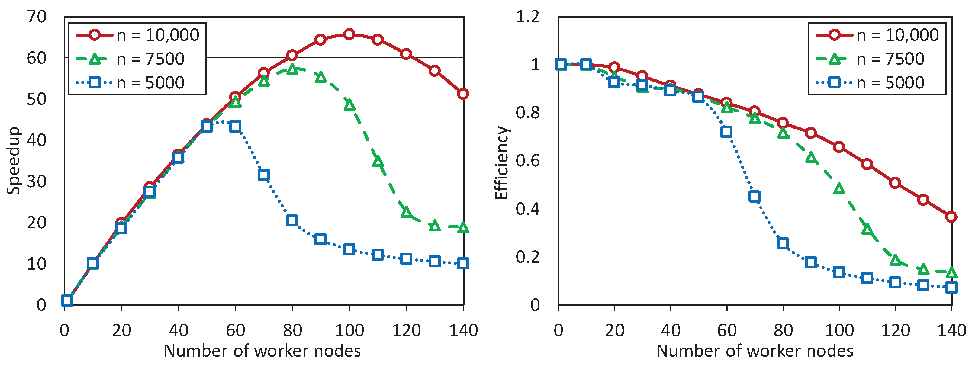
As test problems, we used random synthetic LP problems generated by the program FRaGenLP [52]. A verification of solutions obtained by the apex method was performed using the program VaLiPro [53]. We conducted a series of computational experiments in which we investigated the dependence of speedup and parallel efficiency on the number of worker nodes used. The results are presented in Figure 2.

Here, the speedup $\alpha$ is defined as the ratio of the time $T\left(1\right)$ required by the parallel algorithm using one master node and one worker node to solve a problem to the time $T\left(L\right)$ required by the parallel algorithm using one master node and L worker nodes to solve the same problem:

$$\alpha =\frac{T\left(1\right)}{T\left(L\right)}.$$

(141)

The parallel efficiency $ϵ$ is calculated as the ratio of the speedup $\alpha$ to the number L of worker nodes:

$$ϵ=\frac{\alpha }{L}.$$

(142)

The computations were performed with the following dimensions: 5000, 7500, and 10,000. The number of inequalities was 10,002, 15,002, and 20,002, respectively. The experiments showed that the scalability boundary of the parallel apex algorithm depends significantly on the size of the LP problem. For $n=5000$, the scalability boundary was approximately 55 worker nodes. For the problem of dimension $n=7500$, this boundary increased to 80 nodes, and for the problem of dimension n = 10,000, it was close to 100 nodes. Further increasing the problem size caused the compiler error: “insufficient memory”. It should be noted that the computations were performed in the double double-precision floating-point format occupying 64 bits in computer memory. An attempt to use the single-precision floating-point format occupying 32 bits failed because the apex algorithm stopped to convergeconverging. Parallel efficiency also significantly depends on the size of the LP problem. For $n=5000$, the efficiency dropped below 50% at 70 worker nodes. For $n=7500$ and n = 10,000, the 50% drop of the efficiency occurred at 110 and 130 worker nodes, respectively.

The experiments have also shown that the parameter $\eta$ used in Equation (117) to calculate the apex point z at the quest stage has a negligible effect on the total time of solving the problem when this parameter has large values (more then than 100,000). If the apex point is not far enough away from the polytope, then its pseudoprojection-projection can be an interior point of some polytope face. If the apex point is taken far enough away from the polytope (the value $\eta =20,000·n$ was used in the experiments), then the pseudoprojection-projection always fell into one of the polytope vertices. AlsoAdditionally, we would like to note that, in the case of synthetic LP problems generated by the program FRaGenLP, all computed points in the sequence $\left\{u^{\left(k\right)}\right\}$ were vertices of the polytope. The computational experiment showed that more than 99% of the time spent for solving the LP problem by the apex method was taken up by the calculation of pseudoprojections (Step 18 of Algorithm 3). At that, theThe calculation of one approximation $u^{\left(k\right)}$ for a problem of dimension n = 10,000 on 100 worker nodes took 44 min.

We also tested the apex method on a subset of LP problems from the Netlib-LP repository [54] available at https://netlib.org/lp/data (accessed on 1 March 2023). The Netlib suite of linear optimization problems includes many real real-world applications like such as stochastic forestry problems, oil refinery problems, flap settings of aircraft, pilot models, audit staff scheduling, truss structure problems, airline schedule planning, industrial production, and allocation models, image restoration problems, and multisector economic planning problems. It contains problems ranging in size from 32 variables and 27 constraints up to 15,695 variables and 16,675 constraints [55]. The exact solutions (optimal values of objective functions) of all problems were obtained from paper [56]. The results are presented in

Table 2. Applying the apex method to the Netlib-LP problems.

No	Problem		Quest Stage		Target Stage
	Name	Exact Solution	Rough Solution	Error	Refined Solution	Error
1	adlittle	$2.25494963\times {10}^5$	$3.67140280\times {10}^5$	$6.28\times {10}^{-1}$	$2.2571324\times {10}^5$	$9.68\times {10}^{-4}$
2	afiro	$-4.64753142\times {10}^2$	$-4.55961488\times {10}^2$	$1.89\times {10}^{-2}$	$-4.6475310\times {10}^2$	$8.61\times {10}^{-9}$
3	blend	$-3.08121498\times {10}^1$	$-3.60232513\times {10}^0$	$8.83\times {10}^{-1}$	$-3.0811018\times {10}^1$	$3.19\times {10}^{-5}$
4	fit1d	$-9.14637809\times {10}^3$	$-3.49931014\times {10}^3$	$6.17\times {10}^{-1}$	$-9.1463386\times {10}^3$	$8.77\times {10}^{-7}$
5	kb2	$-1.74990012\times {10}^3$	$-1.39603193\times {10}^3$	$2.02\times {10}^{-1}$	$-1.6879152\times {10}^3$	$3.54\times {10}^{-2}$
6	recipe	$-2.66616000\times {10}^2$	$-2.66107349\times {10}^2$	$1.91\times {10}^{-3}$	$-2.6660404\times {10}^2$	$2.23\times {10}^{-5}$
7	sc50a	$-6.45750770\times {10}^1$	$-5.58016335\times {10}^1$	$1.36\times {10}^{-1}$	$-6.4568167\times {10}^1$	$1.06\times {10}^{-4}$
8	sc50b	$-7.00000000\times {10}^1$	$-6.92167246\times {10}^1$	$1.12\times {10}^{-2}$	$-6.9990792\times {10}^1$	$1.32\times {10}^{-4}$
9	sc105	$-5.22020612\times {10}^1$	$-4.28785710\times {10}^1$	$1.79\times {10}^{-1}$	$-5.1837995\times {10}^1$	$6.97\times {10}^{-3}$
10	share2b	$-4.15732240\times {10}^2$	$-4.28792528\times {10}^2$	$3.14\times {10}^{-2}$	$-4.1572001\times {10}^2$	$2.40\times {10}^{-5}$

.

These experiments showed that the relative error of the rough solution calculated at the quest stage was less than or equal to 0.2, excluding the adlittle, blend, and fit1d problems. The relative error of the refined solution calculated at the target stage was less than ${10}^{-3}$, excluding the kb2 and sc105, for which the error was $0.035$ and $0.007$, respectively. The runtime varied from a few seconds for afiro to tens of hours for blend. One of the main parameters affecting the convergence rate of the apex method was the parameter $ϵ$ used in Step 12 of the parallel Algorithm 2 calculating the pseudoprojection. All runs are available on https://github.com/leonid-sokolinsky/Apex-method/tree/master/Runs (accessed on 1 March 2023).

6. Discussion

In this section of the article, we will discuss some issues related to the scientific contribution and applicability of the apex method in practice and give answers to the following questions.

1.

What is the scientific contribution of this article?

2.

What is the practical significance of the apex method?

3.

What is our confidence that the apex method always converges to the exact solution of the LP problem?

4.

How can we speed up the convergence of the Algorithm 1 calculating a pseudoprojection on the feasible polytope M?

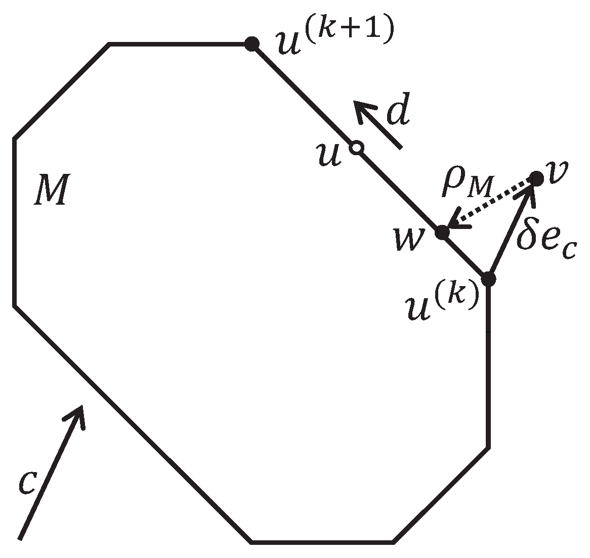
The main scientific contribution of this article is that it presents the apex method that allows, for the first time, as far as we know, to construct a path close to optimal on the surface of a feasible polytope from a certain starting point to the exact solution of the LP problem. Here, the optimal path refers to a path of the minimum length according to the Euclidean metric. By intuition, moving in the direction of the greatest increase in the value of the objective function will give us the shortest path to the point of maximum of the objective function on the surface of the feasible polytope. We intend to present a formal proof of this fact in a futurefuture work.

The practical significance of the apex method is based on the issue of applying feedforward-forward neural networks, including convolutional neural networks, to solve LP problems. In recenta recent paper [28], a method of visual representation of n-dimensional LP problems was proposed. This method constructs an image of the feasible polytope M in the form of a matrix I of dimension $(n-1)$ using the rasterization technique. A vector antiparallel to the gradient vector of the objective function is used as the view ray. Each pixel value in I is proportional to the value of the objective function at the corresponding point on the surface of a feasible polytope M. Such an image makes it possible to use a feedforward neural network to construct the optimal path on the surface of the feasible polytope to the solution of the LP problem. Actually, tThe feedforward neural network can directly calculate the vector d in Algorithm 3, making the calculation of pseudoprojection redundant. The advantage of this approach is that the feedforward-forward neural network works in real time, which is important for robotics. We are not aware of other methods that solvessolve LP problems in real time. However, applying a feedforward neural network to solve LP problems involves the task of preparing a training dataset. The apex method provides the possibility to construct such a training dataset.

Proposition 6 states that Algorithm 3 converges to some point on the surface of the feasible polytope M in a finite number of steps, but leaves open the question of whether the terminal point will be a solution to the LP problem. According to Proposition 8, the answer to this question is positive if, in Algorithm 3, the pseudoprojection is replaced by the metric projection. However, there are no methods for constructing the metric projection for an arbitrarily bounded convex polytope. Therefore, we are forced to use the pseudoprojection. Numerous experiments show that the apex method converges to the solution of the LP problem, but this fact requires a formal proof. We plan to make such a proof in our future work.

The main drawback of the apex method is the slow rate of convergence to the solution of the LP problem. The LP problem, which takes several seconds to find the optimal solution by standard linear programming solvers, may take several hours to solve by the apex method. Computational experiments demonstrated that more than 99% of the time spent for solving the LP problem by the apex method was taken by the calculation of pseudoprojections. Therefore, the issue of speeding up the process of calculating the pseudoprojection is urgent. In the apex method, the pseudoprojection is calculated by Algorithm 1, which belongs to the class of projection-type methods discussed in detail in Section 2. In the case of closed bounded polytope $M\ne \varnothing$, the projection-type methods have a low linear rate of convergence:

$$∥x^{(k+1)}-{\rho }_M\left(x^{\left(0\right)}\right)∥⩽C{q}^k,$$

(143)

where $0<C<\infty$ is some constant, and $q\in (0,1)$ is a parameter that depends on the angles between the half-spaces corresponding to the faces of the polytope M [57]. This means that the distance between adjacent approximations decreases at each iteration by a constant factor of less than 1. For small angles, the convergence rate can decrease todecrease to values close to zero. This fundamental limitation of the projection-type methods cannot be overcome. However, we can reduce the number of half-spaces used to compute the pseudoprojection. According to Proposition 3, the solution of LP problem (38) belongs to some c-recessive half-space. Hence, in Algorithm 1 calculating the pseudoprojection, we can take into account only the c-recessive hyperplanes. On average, this reduces the number of half-spaces by two times. Another way to reduce the pseudoprojection calculation time is to parallelize Algorithm 1, as was done in Algorithm 2. However, the degree of parallelism in this case, in this case, will be limited by the theoretical estimation (115).

7. Conclusions and Future Work

In this paper, we proposed a new scalable iterative method for linear programming called the “apex method”. The key feature of this method is constructing a path close to optimal on the surface of the feasible region from a certain starting point to the exact solution of the linear programming problem. The optimal path refers to a path of the minimum length according to the Euclidean metric. The main practical contribution of the apex method is that it opens the possibility of using feedforward neural networks to solve multidimensional LP problems.

The paper presents a theoretical basis used to construct the apex method. The half-spaces generated by the constraints of the LP problem are considered. These half-spaces form the feasible polytope M, which is a closed bounded set. These half-spaces are divided into two groups with respect to the gradient c of the linear objective function: c-neutral-dominant and c-recessive. The necessary and sufficient condition for the c-recessivity is obtained. It is proved that the solution of to the LP problem lies on the boundary of a c-recessive half-space. The equation defining the apex point not belonging to any c-recessive half-space is derived. The apex point is used to calculate the initial approximation on the surface of the feasible polytope M. The apex method constructs a path close to optimal on the surface of the feasible polytope M from this initial approximation to the solution of the LP problem. To do this, it uses a parallel algorithm constructing the pseudoprojection, which is a generalization of the notion of metric projection. For this parallel algorithm, an analytical estimation of the scalability bound is obtained. This estimation says that the scalability boundary of the parallel algorithm, of calculating the pseudoprojection on a cluster computing system, does not exceed $O\left(\sqrt{m}\right)$ processor nodes, where m is the number of constraints of the linear programming problem. The algorithm constructing a path close to optimal on the surface of the feasible polytope, from the initial approximation to the exact solution of the linear programming problem, is described. The convergence of this algorithm is proven.

The parallel version of the apex method is implemented in C++ using the BSF-skeleton based on the BSF parallel computation model. Large-scale computational experiments were conducted to investigate the scalability of the apex method on a cluster computing system. These experiments show that, for a synthetic scalable linear programming problem with a dimension of 10,000 and a constraint number of 20,002, the scalability boundary of the apex methods is close to 100 processor nodes. At the same time, these experiments showed that more than 99% of the time spent for solving the LP problem by the apex method was taken by the calculation of pseudoprojections.

In addition, the apex method was used to solve 10 problems from the Netlib-LP repository. These experiments showed that the relative error varied from $3.5\times {10}^{-3}$ to $8.6\times {10}^{-9}$. The runtime ranged from a few seconds for to tens of hours. The main parameter affecting the convergence rate of the apex method was the precision of calculating the pseudoprojection.

Our future research directions on this subject are as followingfollows. We plan to develop a new method for calculating the pseudoprojection onto the feasible polytope of the LP problem. The basic idea is to reduce the number of half-spaces used in one iteration. At the same time, the number of these half-spaces should remain large enough to enable the efficient parallelization. The new method should outperform Algorithm 2 in terms of convergence rate. We will also need to prove that the new method converges to a point that lies on the boundary of the feasible region. In addition, we plan to investigate the usefulness of utilizusing the linear superiorization technique [46] in the apex method.

References

1. Sokolinsky, L.B.; Sokolinskaya, I.M. Scalable Method for Linear Optimization of Industrial Processes. In Proceedings of the 2020 Global Smart Industry Conference, GloSIC, Chelyabinsk, Russia, 17–19 November 2020; IEEE: Piscataway, NJ, USA, 2020; pp. 20–26. [Google Scholar] [CrossRef]
2. Jagadish, H.V.; Gehrke, J.; Labrinidis, A.; Papakonstantinou, Y.; Patel, J.M.; Ramakrishnan, R.; Shahabi, C. Big data and its technical challenges. Commun. ACM 2014, 57, 86–94. [Google Scholar] [CrossRef]
3. Hartung, T. Making Big Sense From Big Data. Front. Big Data 2018, 1, 5. [Google Scholar] [CrossRef] [PubMed] [Green Version]
4. Sokolinskaya, I.; Sokolinsky, L.B. On the Solution of Linear Programming Problems in the Age of Big Data. In Proceedings of the Parallel Computational Technologies. PCT 2017. Communications in Computer and Information Science, Kazan, Russia, 3–7 April 2017; Sokolinsky, L., Zymbler, M., Eds.; Springer: Cham, Switzerland, 2017; Volume 753, pp. 86–100. [Google Scholar] [CrossRef] [Green Version]
5. Chung, W. Applying large-scale linear programming in business analytics. In Proceedings of the 2015 IEEE International Conference on Industrial Engineering and Engineering Management (IEEM), Singapore, 6–9 December 2015; IEEE: Piscataway, NJ, USA, 2015; pp. 1860–1864. [Google Scholar] [CrossRef]
6. Gondzio, J.; Gruca, J.A.; Hall, J.A.J.; Laskowski, W.; Zukowski, M. Solving large-scale optimization problems related to Bell’s Theorem. J. Comput. Appl. Math. 2014, 263, 392–404. [Google Scholar] [CrossRef] [Green Version]
7. Sodhi, M.S. LP modeling for asset-liability management: A survey of choices and simplifications. Oper. Res. 2005, 53, 181–196. [Google Scholar] [CrossRef] [Green Version]
8. Branke, J. Optimization in Dynamic Environments. In Evolutionary Optimization in Dynamic Environments. Genetic Algorithms and Evolutionary Computation; Springer: Boston, MA, USA, 2002; Volume 3, pp. 13–29. [Google Scholar] [CrossRef]
9. Brogaard, J.; Hendershott, T.; Riordan, R. High-Frequency Trading and Price Discovery. Rev. Financ. Stud. 2014, 27, 2267–2306. [Google Scholar] [CrossRef] [Green Version]
10. Deng, S.; Huang, X.; Wang, J.; Qin, Z.; Fu, Z.; Wang, A.; Yang, T. A Decision Support System for Trading in Apple Futures Market Using Predictions Fusion. IEEE Access 2021, 9, 1271–1285. [Google Scholar] [CrossRef]
11. Seregin, G. Lecture Notes on Regularity Theory for the Navier-Stokes Equations; World Scientific Publishing Company: Singapore, 2014; p. 268. [Google Scholar] [CrossRef]
12. Demin, D.A. Synthesis of optimal control of technological processes based on a multialternative parametric description of the final state. East. Eur. J. Enterp. Technol. 2017, 3, 51–63. [Google Scholar] [CrossRef] [Green Version]
13. Kazarinov, L.S.; Shnayder, D.A.; Kolesnikova, O.V. Heat load control in steam boilers. In Proceedings of the 2017 International Conference on Industrial Engineering, Applications and Manufacturing, ICIEAM 2017—Proceedings, Saint Petersburg, Russia, 16–19 May 2017; IEEE: Piscataway, NJ, USA, 2017. [Google Scholar] [CrossRef]
14. Zagoskina, E.V.; Barbasova, T.A.; Shnaider, D.A. Intelligent Control System of Blast-furnace Melting Efficiency. In Proceedings of the SIBIRCON 2019—International Multi-Conference on Engineering, Computer and Information Sciences, Proceedings, Novosibirsk, Russia, 21–27 October 2019; IEEE: Piscataway, NJ, USA, 2019; pp. 710–713. [Google Scholar] [CrossRef]
15. Fleming, J.; Yan, X.; Allison, C.; Stanton, N.; Lot, R. Real-time predictive eco-driving assistance considering road geometry and long-range radar measurements. IET Intell. Transp. Syst. 2021, 15, 573–583. [Google Scholar] [CrossRef]
16. Scholl, M.; Minnerup, K.; Reiter, C.; Bernhardt, B.; Weisbrodt, E.; Newiger, S. Optimization of a thermal management system for battery electric vehicles. In Proceedings of the 14th International Conference on Ecological Vehicles and Renewable Energies, EVER, Monte-Carlo, Monaco, 8–10 May 2019; IEEE: Piscataway, NJ, USA, 2019. [Google Scholar] [CrossRef]
17. Meisel, S. Dynamic Vehicle Routing. In Anticipatory Optimization for Dynamic Decision Making. Operations Research/Computer Science Interfaces Series; Springer: New York, NY, USA, 2011; Volume 51, pp. 77–96. [Google Scholar] [CrossRef]
18. Cheng, A.M.K. Real-Time Scheduling and Schedulability Analysis. In Real-Time Systems: Scheduling, Analysis, and Verification; John Wiley and Sons: Hoboken, NJ, USA, 2002; pp. 41–85. [Google Scholar] [CrossRef]
19. Kopetz, H. Real-Time Scheduling. In Real-Time Systems. Real-Time Systems Series; Springer: Boston, MA, USA, 2011; pp. 239–258. [Google Scholar] [CrossRef]
20. Prieto, A.; Prieto, B.; Ortigosa, E.M.; Ros, E.; Pelayo, F.; Ortega, J.; Rojas, I. Neural networks: An overview of early research, current frameworks and new challenges. Neurocomputing 2016, 214, 242–268. [Google Scholar] [CrossRef]
21. Raina, R.; Madhavan, A.; Ng, A.Y. Large-scale deep unsupervised learning using graphics processors. In Proceedings of the 26th Annual International Conference on Machine Learning (ICML’09), Montreal, QC, Canada, 14–18 June 2009; ACM Press: New York, NY, USA, 2009; pp. 873–880. [Google Scholar] [CrossRef] [Green Version]
22. Tank, D.W.; Hopfield, J.J. Simple ‘neural’ optimization networks: An A/D converter, signal decision circuit, and a linear programming circuit. IEEE Trans. Circuits Syst. 1986, CAS-33, 533–541. [Google Scholar] [CrossRef] [Green Version]
23. Kennedy, M.P.; Chua, L.O. Unifying the Tank and Hopfield Linear Programming Circuit and the Canonical Nonlinear Programming Circuit of Chua and Lin. IEEE Trans. Circuits Syst. 1987, 34, 210–214. [Google Scholar] [CrossRef]
24. Rodriguez-Vazquez, A.; Dominguez-Castro, R.; Rueda, A.; Huertas, J.L.; Sanchez-Sinencio, E. Nonlinear Switched-Capacitor “Neural” Networks for Optimization Problems. IEEE Trans. Circuits Syst. 1990, 37, 384–398. [Google Scholar] [CrossRef]
25. Zak, S.H.; Upatising, V. Solving Linear Programming Problems with Neural Networks: A Comparative Study. IEEE Trans. Neural Netw. 1995, 6, 94–104. [Google Scholar] [CrossRef] [PubMed]
26. Malek, A.; Yari, A. Primal–dual solution for the linear programming problems using neural networks. Appl. Math. Comput. 2005, 167, 198–211. [Google Scholar] [CrossRef]
27. Liu, X.; Zhou, M. A one-layer recurrent neural network for non-smooth convex optimization subject to linear inequality constraints. Chaos Solitons Fractals 2016, 87, 39–46. [Google Scholar] [CrossRef]
28. Olkhovsky, N.; Sokolinsky, L. Visualizing Multidimensional Linear Programming Problems. In Proceedings of the Parallel Computational Technologies. PCT 2022. Communications in Computer and Information Science, Dubna, Russia, 29–31 March 2022; Sokolinsky, L., Zymbler, M., Eds.; Springer: Cham, Switzerland, 2022; Volume 1618, pp. 172–196. [Google Scholar] [CrossRef]
29. LeCun, Y.; Bengio, Y.; Hinton, G. Deep learning. Nature 2015, 521, 436–444. [Google Scholar] [CrossRef]
30. Lachhwani, K. Application of Neural Network Models for Mathematical Programming Problems: A State of Art Review. Arch. Comput. Methods Eng. 2020, 27, 171–182. [Google Scholar] [CrossRef]
31. Kaczmarz, S. Angenherte Auflsung von Systemen linearer Gleichungen. Bull. Int. L’Acadmie Pol. Sci. Lett. Cl. Sci. Mathmatiques Nat. Srie A Sci. Mathmatiques 1937, 35, 355–357. [Google Scholar]
32. Kaczmarz, S. Approximate solution of systems of linear equations. Int. J. Control. 1993, 57, 1269–1271. [Google Scholar] [CrossRef]
33. Cimmino, G. Calcolo approssimato per le soluzioni dei sistemi di equazioni lineari. In La Ricerca Scientifica, XVI; Series II, Anno IX, 1; RicercaSci.: Roma, Italy, 1938; pp. 326–333. [Google Scholar]
34. Gastinel, N. Linear Numerical Analysis; Academic Press: New York, NY, USA, 1971; p. ix+341. [Google Scholar]
35. Agmon, S. The relaxation method for linear inequalities. Can. J. Math. 1954, 6, 382–392. [Google Scholar] [CrossRef]
36. Motzkin, T.S.; Schoenberg, I.J. The relaxation method for linear inequalities. Can. J. Math. 1954, 6, 393–404. [Google Scholar] [CrossRef] [Green Version]
37. Censor, Y.; Elfving, T. New methods for linear inequalities. Linear Algebra Appl. 1982, 42, 199–211. [Google Scholar] [CrossRef] [Green Version]
38. De Pierro, A.R.; Iusem, A.N. A simultaneous projections method for linear inequalities. Linear Algebra Appl. 1985, 64, 243–253. [Google Scholar] [CrossRef] [Green Version]
39. Sokolinskaya, I.; Sokolinsky, L. Revised Pursuit Algorithm for Solving Non-stationary Linear Programming Problems on Modern Computing Clusters with Manycore Accelerators. In Supercomputing. RuSCDays 2016. Communications in Computer and Information Science; Voevodin, V., Sobolev, S., Eds.; Springer: Cham, Switzerland, 2016; Volume 687, pp. 212–223. [Google Scholar] [CrossRef]
40. Sokolinskaya, I.M.; Sokolinsky, L.B. Scalability Evaluation of Cimmino Algorithm for Solving Linear Inequality Systems on Multiprocessors with Distributed Memory. Supercomput. Front. Innov. 2018, 5, 11–22. [Google Scholar] [CrossRef] [Green Version]
41. Sokolinsky, L.B.; Sokolinskaya, I.M. Scalable parallel algorithm for solving non-stationary systems of linear inequalities. Lobachevskii J. Math. 2020, 41, 1571–1580. [Google Scholar] [CrossRef]
42. Gonzalez-Gutierrez, E.; Todorov, M.I. A relaxation method for solving systems with infinitely many linear inequalities. Optim. Lett. 2012, 6, 291–298. [Google Scholar] [CrossRef]
43. Vasin, V.V.; Eremin, I.I. Operators and Iterative Processes of Fejer Type. Theory and Applications; Inverse and III-Posed Problems Series; Walter de Gruyter: Berlin, Germany; New York, NY, USA, 2009; p. 155. [Google Scholar] [CrossRef]
44. Eremin, I.I.; Popov, L.D. Fejer processes in theory and practice: Recent results. Russ. Math. 2009, 53, 36–55. [Google Scholar] [CrossRef]
45. Nurminski, E.A. Single-projection procedure for linear optimization. J. Glob. Optim. 2016, 66, 95–110. [Google Scholar] [CrossRef]
46. Censor, Y. Can linear superiorization be useful for linear optimization problems? Inverse Probl. 2017, 33, 044006. [Google Scholar] [CrossRef] [Green Version]
47. Visuthirattanamanee, R.; Sinapiromsaran, K.; Boonperm, A.A. Self-Regulating Artificial-Free Linear Programming Solver Using a Jump and Simplex Method. Mathematics 2020, 8, 356. [Google Scholar] [CrossRef] [Green Version]
48. Gould, N.I. How good are projection methods for convex feasibility problems? Comput. Optim. Appl. 2008, 40, 1–12. [Google Scholar] [CrossRef] [Green Version]
49. Sokolinsky, L.B. BSF: A parallel computation model for scalability estimation of iterative numerical algorithms on cluster computing systems. J. Parallel Distrib. Comput. 2021, 149, 193–206. [Google Scholar] [CrossRef]
50. Sokolinsky, L.B. BSF-skeleton: A Template for Parallelization of Iterative Numerical Algorithms on Cluster Computing Systems. MethodsX 2021, 8, 101437. [Google Scholar] [CrossRef] [PubMed]
51. Dolganina, N.; Ivanova, E.; Bilenko, R.; Rekachinsky, A. HPC Resources of South Ural State University. In Proceedings of the Parallel Computational Technologies. PCT 2022. Communications in Computer and Information Science, Dubna, Russia, 29–31 March 2022; Sokolinsky, L., Zymbler, M., Eds.; Springer: Cham, Switzerland, 2022; Volume 1618, pp. 43–55. [Google Scholar] [CrossRef]
52. Sokolinsky, L.B.; Sokolinskaya, I.M. FRaGenLP: A Generator of Random Linear Programming Problems for Cluster Computing Systems. In Proceedings of the Parallel Computational Technologies. PCT 2021. Communications in Computer and Information Science, Volgograd, Russia, 30 March–1 April 2021; Sokolinsky, L., Zymbler, M., Eds.; Springer: Cham, Switzerland, 2021; Volume 1437, pp. 164–177. [Google Scholar] [CrossRef]
53. Sokolinsky, L.B.; Sokolinskaya, I.M. VaLiPro: Linear Programming Validator for Cluster Computing Systems. Supercomput. Front. Innov. 2021, 8, 51–61. [Google Scholar] [CrossRef]
54. Gay, D.M. Electronic mail distribution of linear programming test problems. Math. Program. Soc. Coal Bull. 1985, 13, 10–12. [Google Scholar]
55. Keil, C.; Jansson, C. Computational experience with rigorous error bounds for the netlib linear programming library. Reliab. Comput. 2006, 12, 303–321. [Google Scholar] [CrossRef] [Green Version]
56. Koch, T. The final NETLIB-LP results. Oper. Res. Lett. 2004, 32, 138–142. [Google Scholar] [CrossRef]
57. Deutsch, F.; Hundal, H. The rate of convergence for the cyclic projections algorithm I: Angles between convex sets. J. Approx. Theory 2006, 142, 36–55. [Google Scholar] [CrossRef]
Figure 1. Iteration execution scheme of the target stage.
Mathematics 11 01654 g001
Figure 2. Speedup and efficiency dependency for various dimensions on the number of worker nodes.
Mathematics 11 01654 g002