

From Zeroing Dynamics to Zeroing-Gradient Dynamics for Solving Tracking Control Problem of Robot Manipulator Dynamic System with Linear Output or Nonlinear Output

Abstract
:1. Introduction
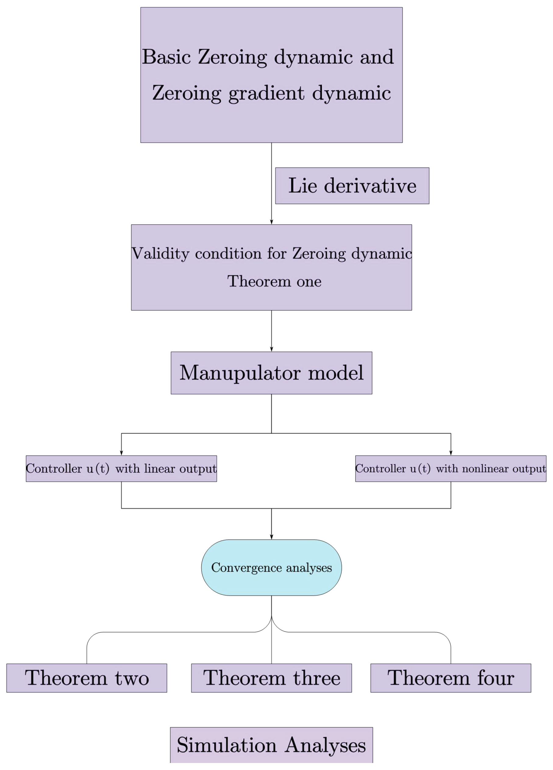
- In the first theorem, the unified formula of the ZD model with order-n with rigorous mathematical proof and its applicable conditions are given by utilizing the Lie derivative.
- The exponential convergence property of the ZD model is given by using the Lie derivative and proved mathematically in the second theorem.
- The steady-state tracking error of the ZGD model is given by the Lie derivative in the third theorem.
- The radius bound where the steady-state tracking error converges exponentially is given in the fourth theorem.
2. Zeroing Dynamics and Zeroing-Gradient Dynamics Models
2.1. Zeroing Dynamics and Zeroing-Gradient Dynamics Models for Tracking Control Problem of Nonlinear System
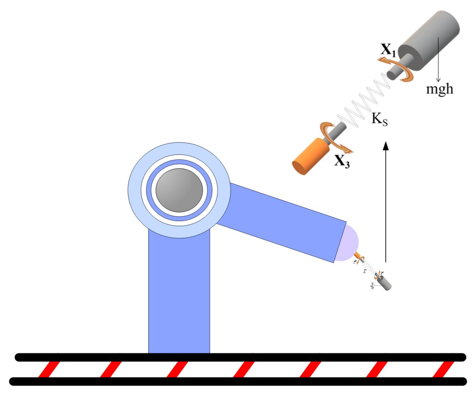
2.2. The Single-Link Manipulator with Flexible Joint Dynamic System
3. Tracking Control of Single-Link Manipulator with Flexible Joints System
3.1. Tracking Control with Single Linear Output of Single-Link Manipulator with Flexible Joints
3.2. Tracking Control with Single Nonlinear Output of Single-Link Manipulator with Flexible Joints
4. Convergence Analyses
- For the situation , if , and , the steady-state tracking error satisfies the following bound condition:
- For the situation , the steady-state tracking error is bounded.
- If , then
- If , then
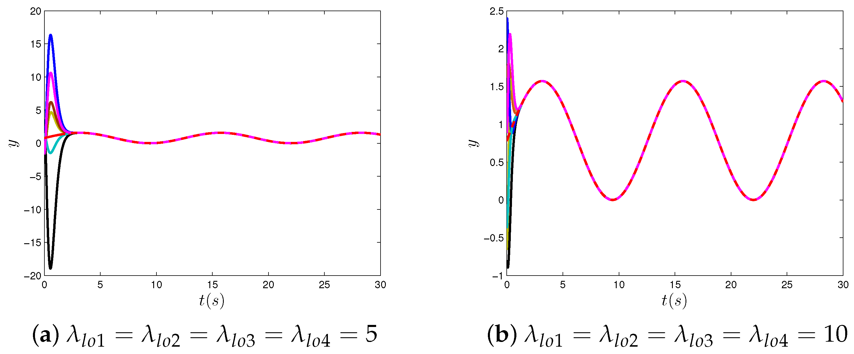
- For the situation , if , and , then, for any loosening parameter , the steady-state tracking error exponentially converges to the closed ball with radius .
- For the situation , the steady-state tracking error is bounded.
- If (i.e., ), then we obtain the following inequality:
- If , then . Therefore, if , then , .
5. Simulations and Discussion
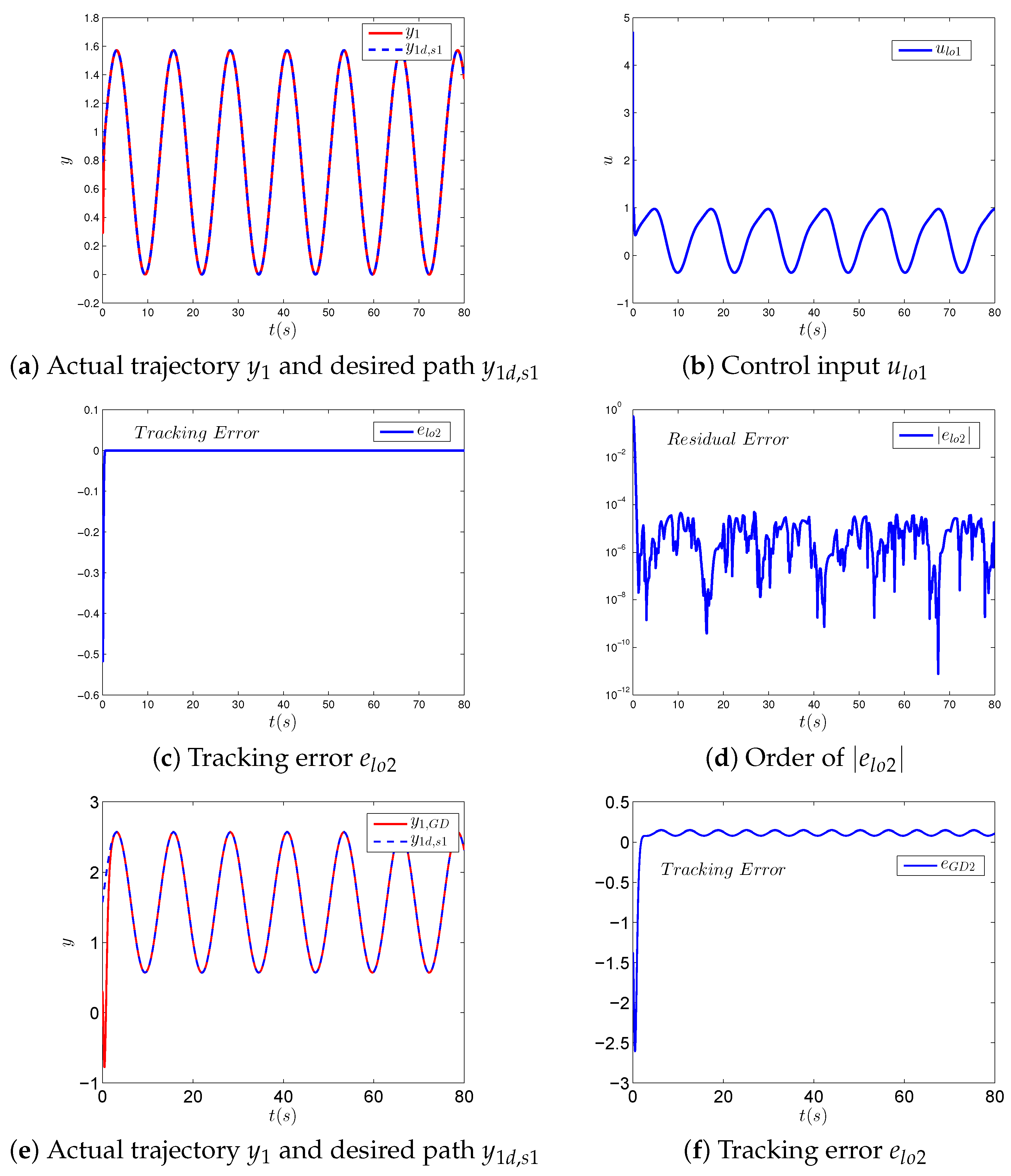
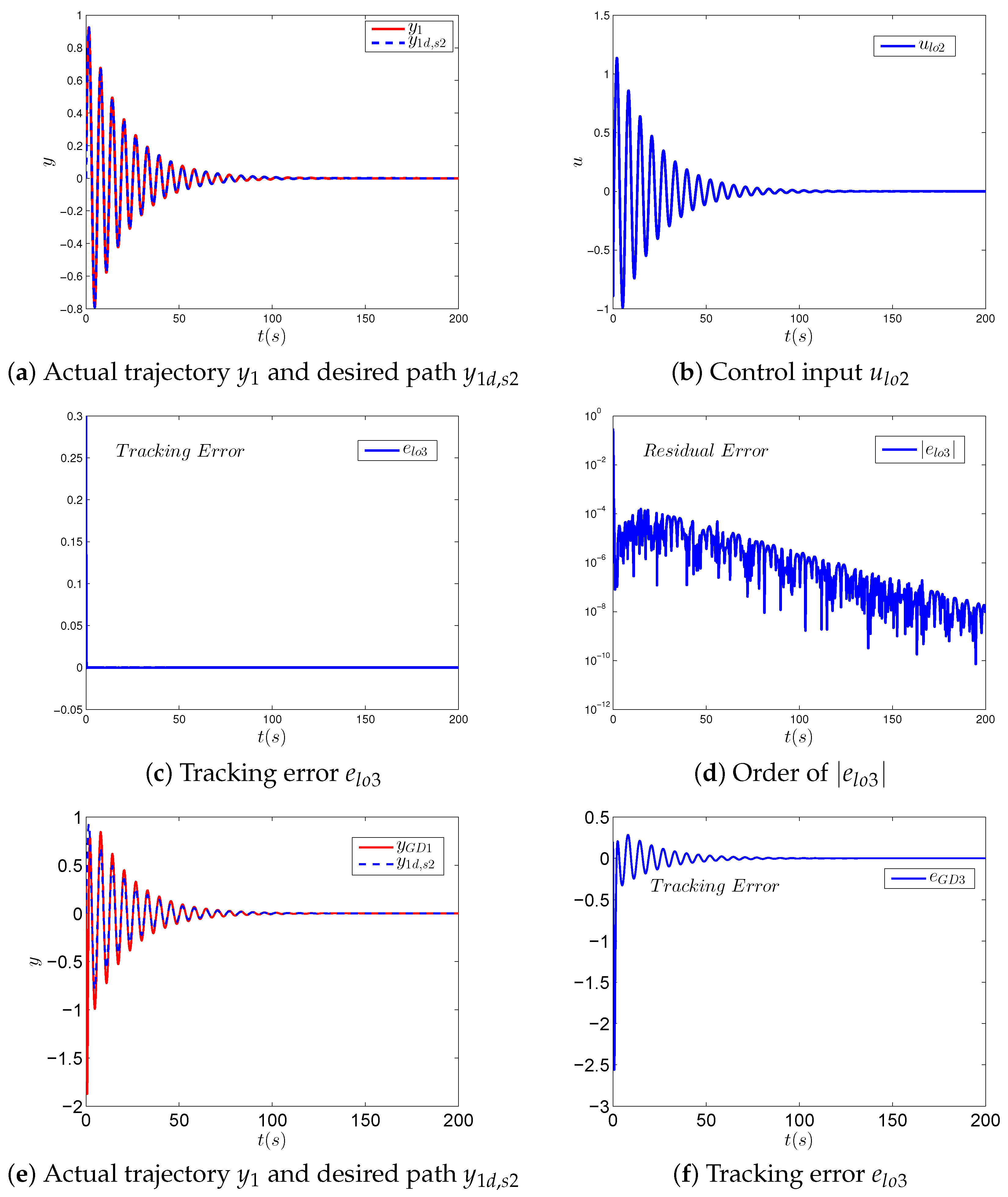
5.1. Test for Tracking Control with Single Linear Output of Single-Link Manipulator with Flexible Joints
5.1.1. Test for Tracking Control with Single Linear Output of Single-Link Manipulator with Flexible Joints in Narrow Space
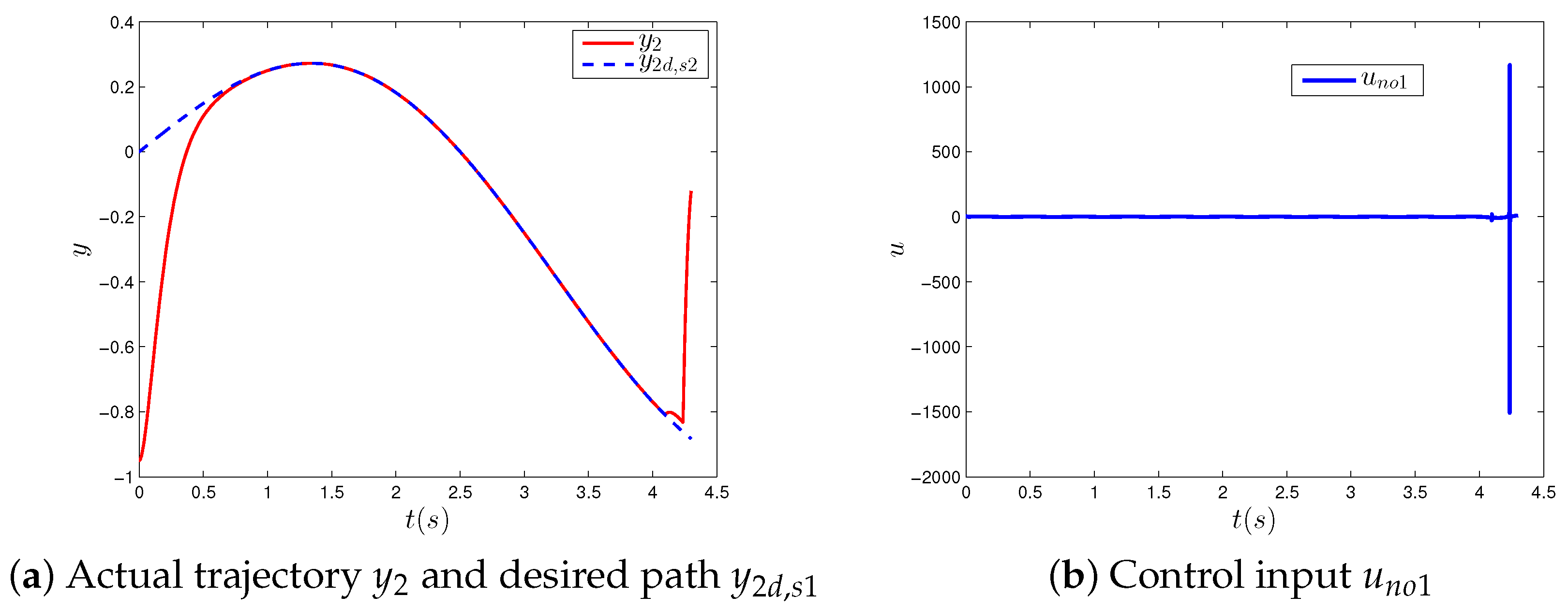
5.1.2. Test for Tracking Control with Single Linear Output of Single-Link Manipulator with Flexible Joints with Application in Calibration
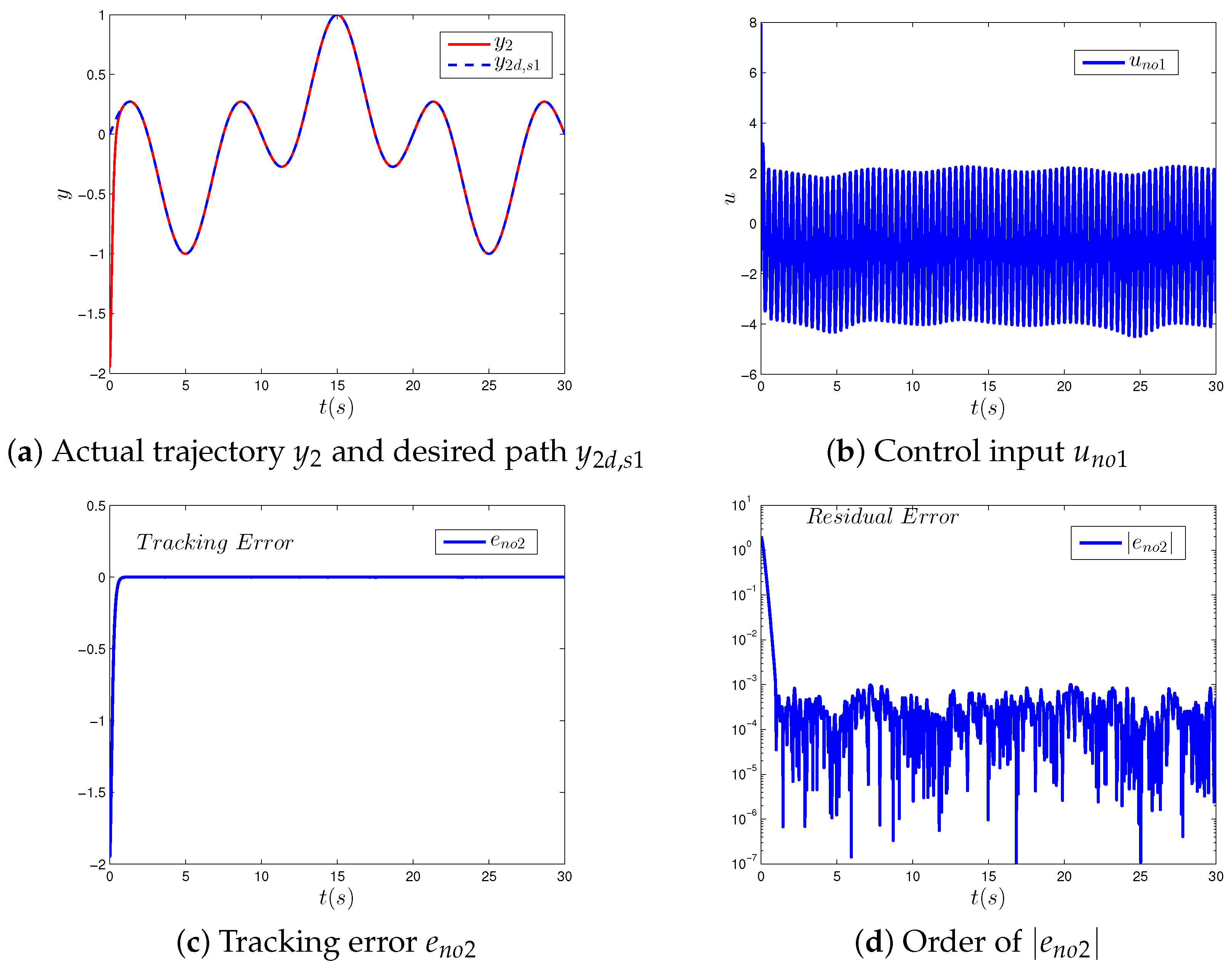
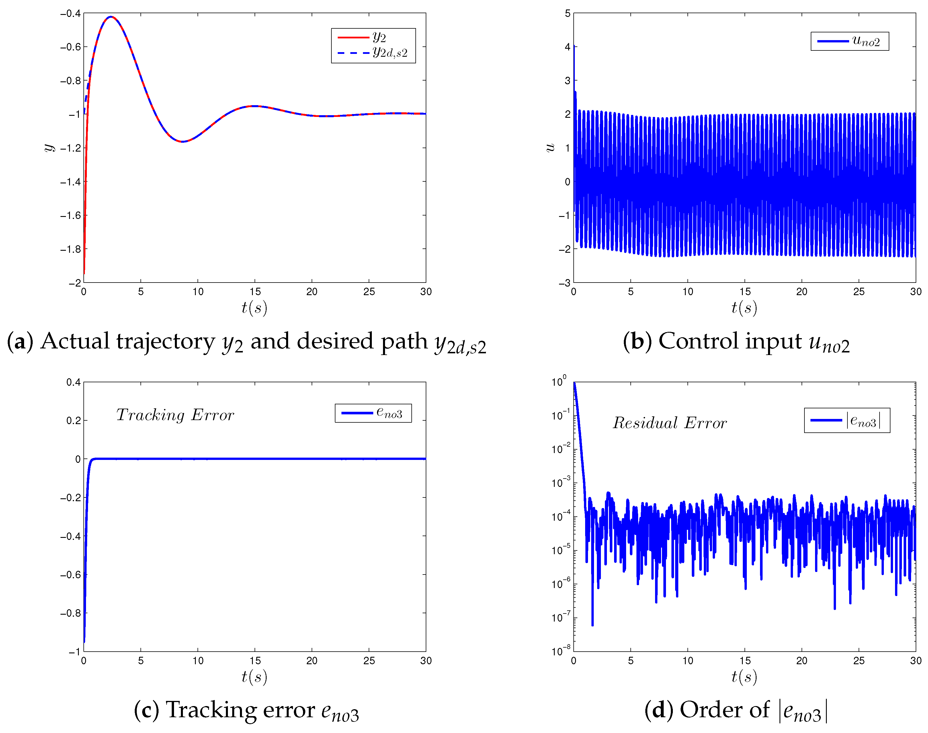
5.2. Test for Tracking Control with Single Nonlinear Output of Single-Link Manipulator with Flexible Joints
6. Conclusions
Author Contributions
Funding
Data Availability Statement
Conflicts of Interest
References
- Kobilarov, M. Nonlinear trajectory control of multi-body aerial manipulators. J. Intell. Robot. Syst. 2014, 73, 679–692. [Google Scholar] [CrossRef]
- Sharma, R.; Tewari, A. Optimal nonlinear tracking of spacecraft attitude maneuvers. IEEE Trans. Control Syst. Technol. 2004, 12, 677–682. [Google Scholar] [CrossRef]
- Khan, M.; Su, H.; Tang, G.-Y. Optimal Tracking Control of Flight Trajectory for Unmanned Aerial Vehicles. In Proceedings of the 2018 IEEE 27th International Symposium on Industrial Electronics (ISIE), Cairns, QLD, Australia, 13–15 June 2018; pp. 264–269. [Google Scholar]
- Tao, X.; Wanger, J.R. An Engine Thermal Management System Design for Military Ground Vehicle—Simultaneous Fan, Pump and Valve Control. SAE Int. J. Passeng. Cars-Electron. Electr. Syst. 2016, 9, 243–254. [Google Scholar] [CrossRef]
- Slotine, J.E.; Li, W. Applied Nonlinear Control; Prentice Hall: Hoboken, NJ, USA, 1991. [Google Scholar]
- Kokotovic, P.V. The joy of feedback: Nonlinear and adaptive. IEEE Control Syst. Mag. 1992, 12, 7–17. [Google Scholar]
- Dorf, R.C.; Bishop, R.H. Modern Control Systems; Addison-Wesley: Glenview, IL, USA, 1995. [Google Scholar]
- Utkin, V.I. Sliding Modes in Control and Optimization; Springer: Berlin/Heidelberg, Germany, 1992. [Google Scholar]
- Johnson, M.A.; Moradi, M.H. PID Control; Springer: Berlin/Heidelberg, Germany, 2005. [Google Scholar]
- Freeman, C.T. Upper Limb Electrical Stimulation Using Input-Output Linearization and Iterative Learning Control. IEEE Trans. Control Syst. Technol. 2015, 23, 1546–1554. [Google Scholar] [CrossRef]
- Nehrir, M.H.; Fatehi, F. Tracking control of DC motors via input-output linearization. Electr. Mach. Power Syst. 1996, 24, 237–247. [Google Scholar] [CrossRef]
- Madani, T.; Benallegue, A. Backstepping control for a quadrotor helicopter. In Proceedings of the IEEE/RSJ International Conference on Intelligent Robots and Systems, Beijing, China, 9–15 October 2006; pp. 3255–3260. [Google Scholar]
- Hua, C.; Liu, P.X.; Guan, X. Backstepping Control for Nonlinear Systems with Time Delays and Applications to Chemical Reactor Systems. IEEE Trans. Ind. Electron. 2009, 56, 3723–3732. [Google Scholar]
- Liu, Y.; Dong, C.Y.; Zhang, W.Q.; Wang, Q. Phase plane design based fast altitude tracking control for hypersonic flight vehicle with angle of attack constraint. Chin. J. Aeronaut. 2021, 34, 490–503. [Google Scholar] [CrossRef]
- Hao, J.G.; Zhang, Y.L. Application of Phase-plane Method in the Co-plane Formation Maintenance of Formation Flying Satellites. In Proceedings of the Chinese Control Conference, Harbin, China, 7–11 August 2006. [Google Scholar]
- Komurcugil, H.; Biricik, S.; Bayhan, S.; Zhang, Z. Sliding mode control: Overview of its applications in power converters. IEEE Ind. Electron. Mag. 2020, 15, 40–49. [Google Scholar] [CrossRef]
- Zhang, Z.; Zhang, K.; Han, Z. Three-dimensional nonlinear trajectory tracking control based on adaptive sliding mode. Aerosp. Sci. Technol. 2022, 128, 107734. [Google Scholar] [CrossRef]
- Xu, Q.; Kan, J.; Chen, S.; Yan, S. Fuzzy PID based trajectory tracking control of mobile robot and its simulation in Simulink. Int. J. Control Autom. 2014, 7, 233–244. [Google Scholar] [CrossRef] [Green Version]
- Loucif, F.; Kechida, S.; Sebbagh, A. Whale optimizer algorithm to tune PID controller for the trajectory tracking control of robot manipulator. J. Braz. Soc. Mech. Sci. Eng. 2020, 42, 1. [Google Scholar] [CrossRef]
- He, C.; Tang, R.; Lam, H.-K.; Cao, J.; Yang, X. Mode-Dependent Event-Triggered Output Control for Switched T-S Fuzzy Systems with Stochastic Switching. IEEE Trans. Fuzzy Syst. 2022. [Google Scholar] [CrossRef]
- Tabuada, P. Event-triggered real-time scheduling of stabilizing control tasks. IEEE Trans. Autom. Control 2007, 52, 1680–1685. [Google Scholar] [CrossRef] [Green Version]
- Heemels, W.P.; Johansson, K.H.; Tabuada, P. An introduction to event-triggered and self-triggered control. In Proceedings of the IEEE 51st IEEE Conference on Decision and Control, Maui, HI, USA, 10–13 December 2012; pp. 3270–3285. [Google Scholar] [CrossRef] [Green Version]
- Wang, H.; Yang, X.; Xiang, Z.; Tang, R.; Ning, Q. Synchronization of Switched Neural Networks via Attacked Mode-Dependent Event-Triggered Control and Its Application in Image Encryption. IEEE Trans. Cybern. 2022. [Google Scholar] [CrossRef]
- Li, S.; Zhou, M.; Yu, X. Design and Implementation of Terminal Sliding Mode Control Method for PMSM Speed Regulation System. IEEE Trans. Ind. Inform. 2013, 9, 1879–1891. [Google Scholar] [CrossRef]
- Sung, S.W.; Lee, I.B. Limitations and countermeasures of PID controllers. Ind. Eng. Chem. Res. 1996, 35, 596–2610. [Google Scholar] [CrossRef]
- Xie, L.L.; Guo, L. Fundamental limitations of discrete-time adaptive nonlinear control. IEEE Trans. Autom. Control 1999, 44, 1777–1782. [Google Scholar]
- Bishop, C.M. Neural networks and their applications. Rev. Sci. Instrum. 1994, 65, 1803–1832. [Google Scholar] [CrossRef] [Green Version]
- Man, Z.; Wu, H.R.; Palaniswami, M. An adaptive tracking controller using neural networks for a class of nonlinear systems. IEEE Trans. Neural Netw. 1998, 9, 947–955. [Google Scholar]
- Broomhead, D.S.; Lowe, D. Radial Basis Functions, Multi-Variable Functional Interpolation and Adaptive Networks; Royal Signals and Radar Establishment: Malvern, UK, 1988. [Google Scholar]
- Zheng, D.; Pan, Y.; Guo, K.; Yu, H. Identification and Control of Nonlinear Systems Using Neural Networks: A Singularity-Free Approach. IEEE Trans. Neural Netw. Learn. Syst. 2019, 30, 2696–2706. [Google Scholar] [CrossRef]
- Kumar, N.; Panwar, V.; Sukavanam, N.; Sharma, S.P.; Borm, J.H. Neural network-based nonlinear tracking control of kinematically redundant robot manipulators. Math. Comput. Model 2011, 53, 1889–1901. [Google Scholar] [CrossRef]
- Muñoz, F.; Cervantes-Rojas, J.S.; Valdovinos, J.M.; Sandre-Hernández, O.; Salazar, S.; Romero, H. Dynamic Neural Network-Based Adaptive Tracking Control for an Autonomous Underwater Vehicle Subject to Modeling and Parametric Uncertainties. Appl. Sci. 2021, 11, 2797. [Google Scholar] [CrossRef]
- Zhang, Y.; Qiu, B.; Li, X. Zhang-Gradient Control; Springer: Singapore, 2021. [Google Scholar]
- Zhang, Y.; Yi, C. Zhang Dynamicss and Neural-Dynamic Method; Nova Science Publishers: New York, NY, USA, 2011. [Google Scholar]
- Zhang, Y.; Yi, C.; Guo, D.; Zheng, J. Comparison on zhang neural dynamics and gradient based neural dynamics for online solution of nonlinear time-varying equation. Neural Comput. Appl. 2011, 20, 1–7. [Google Scholar] [CrossRef]
- Zhang, Y.; Yin, Y.; Wu, H.; Guo, D. Zhang Dynamics and Gradient Dynamics with Tracking-Control Application. In Proceedings of the Fifth International Symposium on Computational Intelligence and Design, Hangzhou, China, 28–29 October 2012. [Google Scholar]
- Li, J.; Mao, M.; Zhang, Y. Simpler ZD-achieving controller for chaotic systems synchronization with parameter perturbation, model uncertainty and external disturbance as compared with other controllers. Optik 2017, 131, 364–373. [Google Scholar] [CrossRef]
- Hu, C.; Guo, D.; Kang, X.; Zhang, Y. Zhang dynamics tracking control of varactor system with stability analysis. In Proceedings of the 2017 13th International Conference on Natural Computation, Fuzzy Systems and Knowledge Discovery (ICNC-FSKD), Guilin, China, 29–31 July 2017; pp. 166–171. [Google Scholar] [CrossRef]
- Li, S.; Chen, S.; Liu, B. Accelerating a recurrent neural network to finite-time convergence for solving time-varying Sylvester equation by using a sign-bi-power activation function. Neural Process. Lett. 2013, 37, 189–205. [Google Scholar] [CrossRef]
- Li, Z.; Yang, M.; Zhang, Y.; Hu, C.; Kang, X. Zhang Neural Dynamics (ZND) Tracking Control of Multiple Integrator Systems with Noise Disturbances: Theoretical and Simulative Results. In Proceedings of the 2020 12th International Conference on Advanced Computational Intelligence (ICACI), Dali, China, 14–16 August 2020; pp. 1–7. [Google Scholar] [CrossRef]
- Groves, K.; Serrani, A. Modeling and Nonlinear Control of a Single-Link Flexible Joint Manipulator. 2004. Available online: http://www.eleceng.ohio-state.edu/~passino/lab5prelab.pdf (accessed on 12 January 2023).
- Hairer, E.; Wanner, G. Solving Ordinary Differential Equations II; Springer: Berlin, Germany, 1991. [Google Scholar]
- Pearson, D. Calculus and Ordinary Differential Equations; Butterworth Heinemann: Oxford, UK, 1995. [Google Scholar]


| Variable Name | Parameter | Value |
|---|---|---|
| Spring Stiffness | 1.61 [N/m] | |
| Inertia of hub | 0.0021 [Kgm2] | |
| Load Inertia | 0.0059 [Kgm2] | |
| Motor Const. | 0.00767 [N/rad/s] | |
| Gear Ratio | 70 | |
| Motor Resist. | 2.6 [] | |
| Link Mass | m | 0.403 [Kg] |
| Grav. Const. | g | −9.81 [N/m] |
| Height of C.M. | h | 0.06 [m] |
Disclaimer/Publisher’s Note: The statements, opinions and data contained in all publications are solely those of the individual author(s) and contributor(s) and not of MDPI and/or the editor(s). MDPI and/or the editor(s) disclaim responsibility for any injury to people or property resulting from any ideas, methods, instructions or products referred to in the content. |
© 2023 by the authors. Licensee MDPI, Basel, Switzerland. This article is an open access article distributed under the terms and conditions of the Creative Commons Attribution (CC BY) license (https://creativecommons.org/licenses/by/4.0/).
Share and Cite
Zheng, Z.; Zeng, D. From Zeroing Dynamics to Zeroing-Gradient Dynamics for Solving Tracking Control Problem of Robot Manipulator Dynamic System with Linear Output or Nonlinear Output. Mathematics 2023, 11, 1605. https://doi.org/10.3390/math11071605
Zheng Z, Zeng D. From Zeroing Dynamics to Zeroing-Gradient Dynamics for Solving Tracking Control Problem of Robot Manipulator Dynamic System with Linear Output or Nonlinear Output. Mathematics. 2023; 11(7):1605. https://doi.org/10.3390/math11071605
Chicago/Turabian StyleZheng, Zheng, and Delu Zeng. 2023. "From Zeroing Dynamics to Zeroing-Gradient Dynamics for Solving Tracking Control Problem of Robot Manipulator Dynamic System with Linear Output or Nonlinear Output" Mathematics 11, no. 7: 1605. https://doi.org/10.3390/math11071605