Effect of Thermal Radiation and Variable Viscosity on Bioconvective and Thermal Stability of Non-Newtonian Nanofluids under Bidirectional Porous Oscillating Regime

Abstract

The bioconvective flow of a Jeffrey fluid conveying tiny particles under the effect of an oscillating stretched bidirectional surface is considered in this paper. The effects of thermal radiation and a porous medium are also investigated. The Cattaneo–Christov diffusion theories are used to analyze the heat and mass transfer phenomena. The activation energy effects are included in the concentration equation. The solved dimensionless equations system is established, based on non-dimensional variables. The analytical findings are evaluated using the homotopic analysis technique. The convergence of solutions is ensured. The results are validated by already available published findings and a good concordance is encountered. The fundamental physical aspect of flow parameters is graphically evaluated. The main results reveal that the velocity is reduced by increasing the permeability of the porous medium. An increase in the temperature occurs when the viscosity of the fluid is varied. The obtained results can be useful in thermal systems, energy production, heat transfer devices, solar systems, biofuels, fertilizers, etc.

1. Introduction

A nanofluid represents a suspension of nanoparticles in a base fluid. These new kinds of engineered fluids are characterized by their enhanced thermophysical properties. Several studies have been performed on the enhancement of thermal processes using nanofluids. Nanofluids can be used to improve the heat transfer in various engineering systems, such as energy production, extrusion processes, solar systems, etc. The first research on nanofluids was performed by Choi [1]. Boungrino [2] reported the thermophoretic and Brownian motion of a nanofluid model. Mahmud et al. [3] investigated the effect of the Lorentz force on the cross-diffusion flow of a couple stress nanofluid over a porous Riga plate. It was mentioned that the Lorentz force effectively controls the fluid flow and enhances the heat transfer. Madkhali et al. [4] studied the mixed convective heat transfer of the Maxwell hybrid nanofluid using the generalized Fourier and Fick laws. The main findings reveal that the rate of the heat transfer is more important using a hybrid nano-Maxwell fluid compared to the pure Maxwell fluid. Hameed et al. [5] studied the combined effects’ heat generation/absorption, magnetic field, and viscous dissipation on the couple stress Casson hybrid nanofluid flow across a nonlinear stretching surface. A reduction in the fluid velocity is noticed when the coupled stress fluid parameter is increased. Chandrasekaran et al. [6] performed an experimental study on the heavy-duty engine radiator with the use of a cerium oxide nanofluid. It was observed that the heat transfer capability of automobile radiators was improved with the use of a cerium oxide-based nanofluid. This improves the radiator performances and engine efficiency by enhancing the heat exchange. Cui et al. [7] investigated the effects of non-identical modeling for a forced convection study of the nanofluid flow across stretching sheets under the effects of a chemical reaction and heat generation. It was found that the heat generation increases the heat transfer more compared to the chemical reaction. Mishra et al. [8] considered the buoyancy-driven flow of a non-Newtonian nanofluid around a moving sphere. It was observed that a separation in velocity is associated to the pulsating flow. Mahmud et al. [9] studied the nanofluid flow with magnetic shear thinning and Hall current effects. The solution of the governing equation was predicted based on the zero-mass flux constraints. A fluctuation in the oblique stagnation point flow was noticed when the ion-slip and Hall effects are considered. Balaji et al. [10] examined the enhanced heat transfer properties of water-based hybrid nanofluids containing multiwall carbon nanotubes and graphene nanoplatelets. It was found that the heat transfer rate was more important for graphene nanoplatelets. Manohar et al. [11] considered the dynamics of the hybrid nanofluid passing through a porous, semi-sphere-shaped fin under the effect of internal heat production. Chen et al. [12] investigated the natural convection of nanofluids under the influence of a variable-direction electrical field. Zheng et al. analyzed the heat transfer and fluid flow corrugated double-tube heat exchanger working with nanofluids. The results show that the use of nanoparticles has significant potential to improve the thermal performance of double-tube heat exchangers. Jaafar et al. [13] discussed the opposing flow phenomenon with a porous space subject to the hybrid nanofluid. Mustafa et al. [14] highlighted the applications of nanofluids in the cooling of LEDs with the help of heat exchangers. Zainal et al. [15] classified the hybrid nanofluid thermal outcomes via numerical simulations. The parallel surface flow with an injection impact due to the interaction of nanoparticles has been focused on by Abdollahi et al. [16].

The phenomenon known as bioconvection is the macroscopic convective motions caused by density variations in a suspension of swimming microorganisms. These motile bacteria can be categorized as oxytactic, gyrotactic, chemotactic, or gravitactic, depending on the cause to which the movement of the bacterium is a response. The process intensification involving correct mixing caused by the thermo-fluidic transport process and mass transfer rate occurs in several industries and in medical science. Shahzad et al. [17] studied the bioconvective micropolar nanofluid flow between double discs with the Cattaneo–Christov heat flux, which is affected by Brownian motion and thermophoretic diffusion. Kairi et al. [18] studied the thermo-solutal Marangoni bioconvective flow of gyrotactic bacteria suspended in a Williamson nanofluid. It was concluded that a higher heat transfer rate occurs when the Marangoni parameter is increased. Hussain et al. [19] investigated the bioconvection of oxytactic microorganisms suspended with a nano-encapsulated phase change material in a porous enclosure. Din et al. [20] studied the bioconvective heat transfer of nanofluid over a moving wedge. Mariam et al. [21] numerically investigated the heat transfer and flow fluid of a nanofluid suspended with microorganisms. Cui et al. [22] studied the bioconvection flow of Oldroyd-B fluid over a flat surface under the effects of a chemical reaction and heat generations. Habib et al. [23] studied the bioconvection and mass transpiration of micropolar nanofluids over an extended surface with a focus on the thermal radiation effect. It was mentioned that a higher Peclet number leads to the reduction in the microorganism’s concentration. Waqas et al. [24] investigated the bioconvective flow of a Casson nanofluid over a spinning disc while considering the slip effects. It was concluded that the presence of slip features enhances the heat transfer considerably.

The non-Newtonian fluids are inspired materials with a novel and complex rheology. The dynamic of such non-Newtonian materials is interesting and unique. Different applications of such materials are predicted in biological systems, chemical industries, mechanical systems, food industries, and manufacturing systems. Moreover, the non-Newtonian fluids are of marvelous importance in cosmetics, medicines, wire drawing, plastic processes, blood, etc. Due to the specified rheology, different constitutive equations are presented to justify the non-Newtonian models. The Jeffrey fluid model is one famous model which attracted the attention of researchers in recent years. The rheology of the Jeffrey model is associated to three factors, namely the viscosity, relaxation to retardation time ratio, and retardation time factor. The Jeffrey fluid model captured the memory features and elastic effects associated to the dilute polymer solutions [25]. The constitutive relation for this model is presented via extra stress tensor $\mathbf{S}$ as

$$\mathbf{S}=\frac{\mu }{\left(1+\mathsf{\Omega }\right)}\left[\mathbf{A}+{\alpha }_{\ast }\left(\frac{\partial \mathbf{A}}{\partial t}+\left(\mathbf{V}·\nabla \right)\mathbf{A}\right)\right],$$

(1)

With material dynamic viscosity $\left(\mu \right),$ retardation time factor $\left({\alpha }_{\ast }\right)$, and relaxation to retardation times ratio $\left(\mathsf{\Omega }\right)$. The scientists have performed different studies by using the Jeffrey fluid model. Muzara and Shateyi [26] tested the viscous dissipation impact for the Jeffrey fluid with the heat source impact. Raje et al. [27] reported the optimized estimation for a pipe flow with Jeffrey material. Khan et al. [28] worked out analytical computations for the Jeffrey fluid flow by using the latest Prabhakar scheme. The thermo-diffusion phenomenon for the Jeffrey material confining the unsteady flow was reported by Mushtaq et al. [29]. Ahmad et al. [30] discussed the three-dimensional flow of the Jeffrey nanofluid with an oscillating regime.

Based on the above presented literature review, it can be concluded that the bioconvective flow of nanofluids has been the subject of several studies. However, the investigation of the bioconvection of the Jeffrey fluid conveying tiny particles in view of variable thermal conductivity has not been reported yet. In the current study, the flow is induced by a bidirectional oscillatory stretching surface instead of a linearly stretched surface. To avoid the turbulent phenomenon, the magnitude of the oscillations was kept small. In addition, the effects of the porous medium and thermal radiation are depicted. The motivations for considering the Jeffrey nanofluid are due to its important rheological features as well as its potential industrial and engineering applications. The formulated problem is solved with the homotopy analysis method. The physical dynamics of this problem are presented via different tables and graphs.

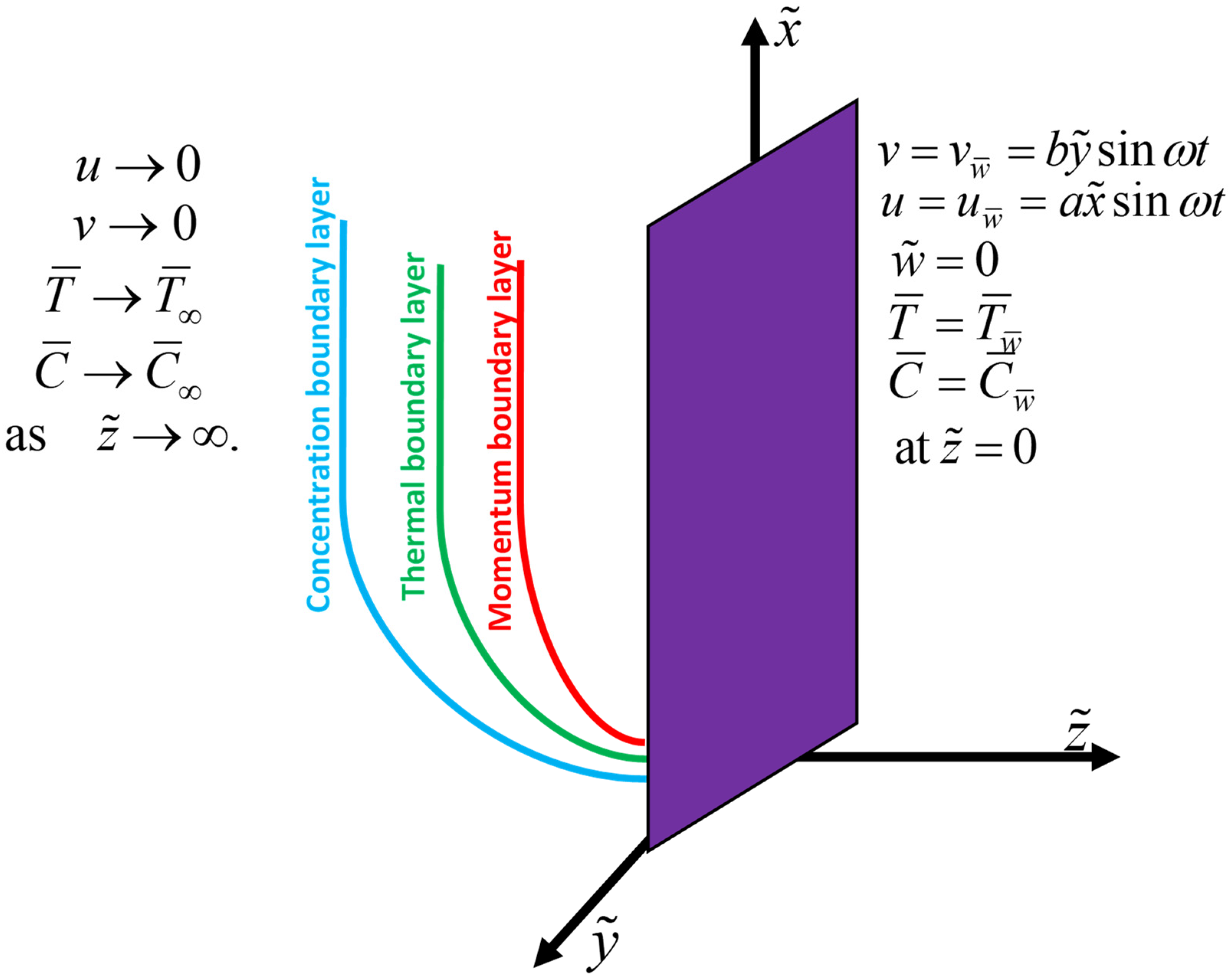
2. Problem Formulation

An unsteady bidirectional flow caused by periodically moving porous surface of Jeffrey fluid conveying tiny particles is considered. The flow is induced by a periodically moving surface having bidirectional velocities $u={/\mathrm{U}}_{\overline{w}}=a\tilde{x}\sin \omega t$ and $v={/\mathrm{V}}_{\overline{w}}=b\tilde{y}\sin \omega t$ along with $\tilde{x}-$ and $\tilde{y}-$directions, respectively (Figure 1). Here, $a,b$ are the stretching rates while the $\omega$ indicates the angular frequency. The unsteady flow is induced by periodically moving surface at $\tilde{z}\ge 0$. The thermal conductivity of the fluid is assumed to be variable. The analysis of thermal and mass transfer features is based on the modified diffusion theories. The thermal radiation effect is also considered in the heat equation. The concentration equation is modified by using the activation energy features by using the Arrhenius equation. Additionally, the moving surface is maintained at a uniform temperature ${\overline{T}}_{\overline{w}},$ microorganisms’ density ${\overline{\mathrm{N}}}_{\overline{w}}$, and nanoparticles concentration ${\overline{C}}_{\overline{w}}$, while microorganisms density, concentration, and the free stream nanofluid temperature are denoted by ${\overline{\mathrm{N}}}_{\infty }, {\overline{C}}_{\infty }, {\overline{T}}_{\infty }$, respectively.

The resulting governing equations are presented as follows [30]:

$$\begin{array}{c}\frac{\partial u}{\partial \tilde{x}}+\frac{\partial v}{\partial \tilde{y}}+\frac{\partial w}{\partial \tilde{z}}=0,\\ \begin{array}{l}\frac{\partial u}{\partial t}+u\left(\frac{\partial u}{\partial \tilde{x}}\right)+v\left(\frac{\partial u}{\partial \tilde{y}}\right)+w\left(\frac{\partial u}{\partial \tilde{z}}\right)=\frac{\nu }{\left(1+\mathsf{\Omega }\right)}\left(\frac{{\partial }^{2}u}{\partial {\tilde{z}}^2}\right)+\frac{\nu {\alpha }_{\ast }}{\left(1+\mathsf{\Omega }\right)}\left(\begin{array}{l}\frac{{\partial }^{3}u}{\partial {\tilde{z}}^2\partial t}+v\frac{{\partial }^{3}u}{\partial \tilde{y}\partial {\tilde{z}}^2}+w\frac{{\partial }^{3}u}{\partial {\tilde{z}}^3}\\ +u\frac{{\partial }^{3}u}{\partial \tilde{x}\partial {\tilde{z}}^2}+\left(\frac{\partial v}{\partial \tilde{z}}\right)\left(\frac{{\partial }^{2}u}{\partial \tilde{y}\partial \tilde{z}}\right)\\ +\left(\frac{\partial u}{\partial \tilde{z}}\right)\left(\frac{{\partial }^{2}u}{\partial \tilde{x}\partial \tilde{z}}\right)+\left(\frac{\partial w}{\partial \tilde{z}}\right)\left(\frac{{\partial }^{2}u}{\partial {\tilde{z}}^2}\right)\end{array}\right)\\ -\frac{\nu u}{k_p}+\frac{g}{{\rho }_{\stackrel{⌢}{f}}}\left[{\rho }_{\stackrel{⌢}{f}}\wp \left(1-{\overline{C}}_{\infty }\right)\left(\overline{T}-{\overline{T}}_{\infty }\right)-\left({\rho }_{\stackrel{⌢}{p}}-{\rho }_{\stackrel{⌢}{f}}\right)\left(\overline{C}-{\overline{C}}_{\infty }\right)-{\sigma }_{\ast }\left({\rho }_{\stackrel{⌢}{m}}-{\rho }_{\stackrel{⌢}{f}}\right)\left(\overline{\mathrm{N}}-{\overline{\mathrm{N}}}_{\infty }\right)\right]\end{array}\end{array}$$

(2)

$$\frac{\partial v}{\partial t}+u\frac{\partial v}{\partial \tilde{x}}+v\frac{\partial v}{\partial \tilde{y}}+w\frac{\partial v}{\partial \tilde{z}}=\frac{\nu }{\left(1+\mathsf{\Omega }\right)}\left(\frac{{\partial }^{2}v}{\partial {\tilde{z}}^2}\right)+\frac{\nu {\alpha }_{\ast }}{\left(1+\mathsf{\Omega }\right)}\left(\begin{array}{l}\frac{{\partial }^{3}v}{\partial {\tilde{z}}^2\partial t}+v\frac{{\partial }^{3}v}{\partial \tilde{y}\partial {\tilde{z}}^2}+w\frac{{\partial }^{3}v}{\partial {\tilde{z}}^3}\\ +\left(\frac{\partial u}{\partial \tilde{z}}\right)\left(\frac{{\partial }^{2}v}{\partial \tilde{x}\partial \tilde{z}}\right)+u\frac{{\partial }^{3}v}{\partial \tilde{x}\partial {\tilde{z}}^2}\\ +\left(\frac{\partial w}{\partial \tilde{z}}\right)\left(\frac{{\partial }^{2}v}{\partial {\tilde{z}}^2}\right)+\left(\frac{\partial v}{\partial \tilde{z}}\right)\left(\frac{{\partial }^{2}v}{\partial \tilde{y}\partial \tilde{z}}\right)\end{array}\right)-\frac{\nu u}{k_p},$$

(3)

$$\begin{array}{l}\frac{\partial \overline{T}}{\partial t}+u\frac{\partial \overline{T}}{\partial \tilde{x}}+v\frac{\partial \overline{T}}{\partial \tilde{y}}+w\frac{\partial \overline{T}}{\partial \tilde{z}}+{\mathsf{\delta }}_{\overline{T}}\left[\begin{array}{l}2u\frac{{\partial }^2\overline{T}}{\partial \tilde{x}\partial t}+w^2\frac{{\partial }^2\overline{T}}{\partial {\tilde{z}}^2}+v^2\frac{{\partial }^2\overline{T}}{\partial {\tilde{y}}^2}+u^2\frac{{\partial }^2\overline{T}}{\partial {\tilde{x}}^2}+2w\frac{{\partial }^2\overline{T}}{\partial \tilde{z}\partial t}+w\frac{\partial u}{\partial \tilde{z}}\frac{\partial \overline{T}}{\partial \tilde{x}}\\ +v\left(\frac{\partial v}{\partial \tilde{y}}\frac{\partial \overline{T}}{\partial \tilde{y}}+\frac{\partial w}{\partial \tilde{y}}\frac{\partial \overline{T}}{\partial \tilde{z}}\right)+u\left(\frac{\partial u}{\partial \tilde{x}}\frac{\partial \overline{T}}{\partial \tilde{x}}+\frac{\partial v}{\partial \tilde{x}}\frac{\partial \overline{T}}{\partial \tilde{y}}+\frac{\partial w}{\partial \tilde{x}}\frac{\partial \overline{T}}{\partial \tilde{z}}\right)\\ +\frac{\partial u}{\partial t}\frac{\partial \overline{T}}{\partial \tilde{x}}+\frac{\partial v}{\partial t}\frac{\partial \overline{T}}{\partial \tilde{y}}+\frac{\partial w}{\partial t}\frac{\partial \overline{T}}{\partial \tilde{z}}+\frac{{\partial }^2\overline{T}}{\partial t^2}+v\frac{\partial u}{\partial \tilde{y}}\frac{\partial \overline{T}}{\partial \tilde{x}}+w\frac{\partial v}{\partial \tilde{z}}\frac{\partial \overline{T}}{\partial \tilde{y}}\\ +2v\left(u\frac{{\partial }^2\overline{T}}{\partial \tilde{x}\partial \tilde{y}}+w\frac{{\partial }^2\overline{T}}{\partial \tilde{y}\partial \tilde{z}}+\frac{{\partial }^2\overline{T}}{\partial \tilde{y}\partial t}\right)+w\left(2u\frac{{\partial }^2\overline{T}}{\partial \tilde{x}\partial \tilde{z}}+\frac{\partial w}{\partial \tilde{z}}\frac{\partial \overline{T}}{\partial \tilde{z}}\right)\end{array}\right]\\ =\frac{1}{{\left(\rho c\right)}_{\stackrel{⌢}{f}}}\frac{\partial }{\partial \tilde{z}}\left(\cancel{k}\left(\overline{T}\right)\frac{\partial \overline{T}}{\partial \tilde{z}}\right)+\frac{16T_{\infty }^3{\sigma }_r}{3{\left(\rho c\right)}_f{k}_r}\frac{{\partial }^2\overline{T}}{\partial y^2}+\mho \left(D_{\overline{B}}\frac{\partial \overline{C}}{\partial \tilde{z}}\frac{\partial \overline{T}}{\partial \tilde{z}}+{\left(\frac{\partial \overline{T}}{\partial \tilde{z}}\right)}^2\frac{D_{\overline{T}}}{{\overline{T}}_{\infty }}\right),\end{array}$$

(4)

$$\begin{array}{l}\frac{\partial \overline{C}}{\partial t}+u\frac{\partial \overline{C}}{\partial \tilde{x}}+v\frac{\partial \overline{C}}{\partial \tilde{y}}+w\frac{\partial \overline{C}}{\partial \tilde{z}}+{\mathsf{\delta }}_{\overline{C}}\left[\begin{array}{l}2u\frac{{\partial }^2\overline{C}}{\partial \tilde{x}\partial t}+w^2\frac{{\partial }^2\overline{C}}{\partial {\tilde{z}}^2}+v^2\frac{{\partial }^2\overline{C}}{\partial {\tilde{y}}^2}+u^2\frac{{\partial }^2\overline{C}}{\partial {\tilde{x}}^2}+2w\frac{{\partial }^2\overline{C}}{\partial \tilde{z}\partial t}+w\frac{\partial u}{\partial \tilde{z}}\frac{\partial \overline{C}}{\partial \tilde{x}}\\ +v\frac{\partial v}{\partial \tilde{y}}\frac{\partial \overline{C}}{\partial \tilde{y}}+u\left(\frac{\partial u}{\partial \tilde{x}}\frac{\partial \overline{C}}{\partial \tilde{x}}+\frac{\partial v}{\partial \tilde{x}}\frac{\partial \overline{C}}{\partial \tilde{y}}+\frac{\partial w}{\partial \tilde{x}}\frac{\partial \overline{C}}{\partial \tilde{z}}\right)+v\frac{\partial w}{\partial \tilde{y}}\frac{\partial \overline{C}}{\partial \tilde{z}}\\ +\frac{\partial u}{\partial t}\frac{\partial \overline{C}}{\partial \tilde{x}}+\frac{\partial v}{\partial t}\frac{\partial \overline{C}}{\partial \tilde{y}}+\frac{\partial w}{\partial t}\frac{\partial \overline{C}}{\partial \tilde{z}}+\frac{{\partial }^2\overline{C}}{\partial t^2}+v\frac{\partial u}{\partial \tilde{y}}\frac{\partial \overline{C}}{\partial \tilde{x}}+w\frac{\partial v}{\partial \tilde{z}}\frac{\partial \overline{C}}{\partial \tilde{y}}\\ +2v\left(u\frac{{\partial }^2\overline{C}}{\partial \tilde{x}\partial \tilde{y}}+w\frac{{\partial }^2\overline{C}}{\partial \tilde{y}\partial \tilde{z}}+\frac{{\partial }^2\overline{C}}{\partial \tilde{y}\partial t}\right)+w\left(2u\frac{{\partial }^2\overline{C}}{\partial \tilde{x}\partial \tilde{z}}+\frac{\partial w}{\partial \tilde{z}}\frac{\partial \overline{C}}{\partial \tilde{z}}\right)\end{array}\right]\\ =D_{\overline{B}}\frac{{\partial }^2\overline{C}}{\partial {\tilde{z}}^2}+\left(\frac{D_{\overline{T}}}{{\overline{T}}_{\infty }}\right)\frac{{\partial }^2\overline{T}}{\partial {\tilde{z}}^2}-{\mathsf{{\rm K}}}_r{}^2\left(\overline{C}-{\overline{C}}_{\infty }\right){\left(\frac{\overline{T}}{{\overline{T}}_{\infty }}\right)}^m\exp \left(\frac{-E_{\odot }}{{\cancel{\beta }}_{\odot }\overline{T}}\right).\end{array}$$

(5)

$$\frac{\partial \overline{\mathrm{N}}}{\partial t}+u\frac{\partial \overline{\mathrm{N}}}{\partial \tilde{x}}+v\frac{\partial \overline{\mathrm{N}}}{\partial \tilde{y}}+w\frac{\partial \overline{\mathrm{N}}}{\partial \tilde{z}}+\frac{\cancel{\Re }\Im }{\left({\overline{C}}_{\overline{w}}-{\overline{C}}_{\infty }\right)}\left[\frac{\partial }{\partial \tilde{z}}\left(\overline{\mathrm{N}}\frac{\partial \overline{C}}{\partial \tilde{z}}\right)\right]=D_{\stackrel{⌢}{m}}\frac{{\partial }^2\overline{\mathrm{N}}}{\partial {\tilde{z}}^2}.$$

(6)

With appropriate boundary constraints [21]:

$$\begin{array}{c}u={/\mathrm{U}}_{\overline{w}}=a\tilde{x}\sin \omega t,\hspace{1em}v={/\mathrm{V}}_{\overline{w}}=b\tilde{y}\sin \omega t,\hspace{1em}\tilde{w}=0,\hspace{1em}\overline{\mathrm{N}}={\overline{\mathrm{N}}}_{\overline{w}},\hspace{1em}\overline{T}={\overline{T}}_{\overline{w}},\hspace{1em}\overline{C}={\overline{C}}_{\overline{w}},\hspace{1em}at\hspace{1em}\tilde{z}=0,\hspace{1em}t>0,\\ u\to 0,\hspace{1em}\frac{\partial u}{\partial \tilde{z}}\to 0,\hspace{1em}v\to 0,\hspace{1em}\frac{\partial v}{\partial \tilde{z}}\to 0,\hspace{1em}\overline{T}\to {\overline{T}}_{\infty },\hspace{1em}\overline{C}\to {\overline{C}}_{\infty },\hspace{1em}\overline{\mathrm{N}}\to {\overline{\mathrm{N}}}_{\infty },\hspace{1em}\mathrm{as}\hspace{1em}\tilde{z}\to \infty .\end{array}\}$$

(7)

With, $\mathsf{\Omega }$, $\nu$, $k_p$, ${\alpha }_{\ast }$, $g$, ${\delta }_{\overline{T}}$, $\wp$, ${\sigma }_{\ast }$, ${\sigma }_r$, $k_r$, $\cancel{k}\left(\overline{T}\right)$, $\mho =\frac{{(\rho c)}_{\stackrel{⌢}{n}}}{{(\rho c)}_{\stackrel{⌢}{f}}}$, $\mathrm{K}$, ${\delta }_{\overline{C}}$, $m$, ${\cancel{\beta }}_{\odot }$, $E_{\odot }$, $\cancel{\Re }$, $\Im$, $\left({\rho }_{\stackrel{⌢}{p}},{\rho }_{\stackrel{⌢}{m}},{\rho }_{\stackrel{⌢}{f}}\right)$ and $\left(D_{\overline{T}},D_{\overline{B}},D_{\stackrel{⌢}{m}}\right)$ represent the ratio of relaxation and delay times; kinematic viscosity; porous medium permeability; retardation time; the gravitational acceleration; thermal relaxation time; thermal expansion coefficient; the microorganisms volume; Stefan Boltzmann constant; Boltzmann constant; thermal conductivity; the heat capacities ratio; reaction rate; solutal relaxation time; the rate constant; activation energy; chemotaxis constant; the swimming cell speed; densities for the nanoparticles, microorganisms, and the base fluid; and diffusivities for thermophoresis, Brownian, and microorganisms, respectively.

In addition, $\cancel{k}\left(\overline{T}\right)$ is expressed as

$$\cancel{k}\left(\overline{T}\right)={\cancel{k}}_{\infty }\left(1+\epsilon \theta \right),$$

(8)

where $\epsilon$ is a small parameter, ${\cancel{k}}_{\infty }$ is the thermal conductivity at the ambient zone, and $\theta$ is the dimensionless temperature.

To obtain the dimensionless expressions, the associated transformations are [21]

$$\begin{array}{c}u=a\tilde{x}{f}_{\xi }(\xi ,\tau ),\hspace{1em}\hspace{1em}\hspace{1em}w=-\sqrt{\nu a}[f(\xi ,\tau )+g(\xi ,\tau )],\hspace{1em}\hspace{1em}v=a\tilde{y}{g}_{\xi }(\xi ,\tau )\hspace{1em}\hspace{1em}\hspace{1em}\tau =t\omega ,\\ \xi =\sqrt{\frac{a}{\nu }}\tilde{z},\hspace{1em}\hspace{1em}\varphi (\xi ,\tau )=\frac{\overline{C}-{\overline{C}}_{\infty }}{{\overline{C}}_{\overline{w}}-{\overline{C}}_{\infty }},\hspace{1em}\hspace{1em}\theta (\xi ,\tau )=\frac{\overline{T}-{\overline{T}}_{\infty }}{{\overline{T}}_{\overline{w}}-{\overline{T}}_{\infty }},\hspace{1em}\hspace{1em}\chi (\xi ,\tau )=\frac{\overline{\mathrm{N}}-{\overline{\mathrm{N}}}_{\infty }}{{\overline{\mathrm{N}}}_{\overline{w}}-{\overline{\mathrm{N}}}_{\infty }}.\end{array}\}$$

(9)

The dimensionless system is

$$\begin{array}{l}{f}_{\xi \xi \xi }-\left(1+\mathsf{\Omega }\right)\left(f_{\xi }{}^2+S{f}_{\xi \tau }-\left(f+g\right)f_{\xi \xi }+\gamma f_{\xi }\right)+\mathsf{\Psi }\left(\begin{array}{l}S{f}_{\xi \xi \xi \tau }-\left(g+f\right)f_{\xi \xi \xi \xi }\\ +f_{\xi \xi }{}^2-g_{\xi }{f}_{\xi \xi \xi }\end{array}\right)\\ +\left(1+\mathsf{\Omega }\right)\left(\mathsf{\varpi }\theta -\mathsf{\varpi }\mathrm{N}\varphi -\mathsf{\varpi }\mathsf{\Pi }\chi \right)=0,\end{array}$$

(10)

$$g_{\xi \xi \xi }-\left(1+\mathsf{\Omega }\right)\left(g_{\xi }{}^2+S{g}_{\xi \tau }-\left(f+g\right)g_{\xi \xi }+\gamma g_{\xi }\right)+\mathsf{\Psi }\left(\begin{array}{l}S{g}_{\xi \xi \xi \tau }-\left(g+f\right)g_{\xi \xi \xi \xi }\\ +g_{\xi \xi }{}^2-f_{\xi }{g}_{\xi \xi \xi }{}_{}\end{array}\right)=0,$$

(11)

$$\begin{array}{l}\left(\frac{1+Rd}{\mathrm{Pr}}\right)\left[\left(1+\epsilon \theta \right){\theta }_{\xi \xi }+\epsilon {\theta }_{\xi }{}^2\right]+\mathrm{Pr}\left(\begin{array}{l}g{\theta }_{\xi }+f{\theta }_{\xi }-S{\theta }_{\tau }+N_t{\theta }_{\xi }{}^2\\ +N_b{\theta }_{\xi }{\varphi }_{\xi }\end{array}\right)\\ -\mathrm{Pr}{\mathsf{\delta }}_1\left(\begin{array}{l}{S}^2{\theta }_{\tau \tau }-S\left(f_{\tau }{\theta }_{\xi }+g_{\tau }{\theta }_{\xi }\right)\\ -2S\left(g+f\right){\theta }_{\tau \xi }+{\left(g+f\right)}^2{\theta }_{\xi \xi }\\ +\left(f_{\xi }+g_{\xi }\right)\left(f+g\right){\theta }_{\xi }\end{array}\right)=0,\end{array}$$

(12)

$$\begin{array}{l}{\varphi }_{\xi \xi }+Sc\left(g{\varphi }_{\xi }+f{\varphi }_{\xi }-S{\varphi }_{\tau }\right)-Sc{\mathsf{\delta }}_2\left(\begin{array}{l}{S}^2{\varphi }_{\tau \tau }-S\left(f_{\tau }{\varphi }_{\xi }+g_{\tau }{\varphi }_{\xi }\right)\\ -2S\left(g+f\right){\varphi }_{\tau \xi }+{\left(g+f\right)}^2{\varphi }_{\xi \xi }\\ +\left(f_{\xi }+g_{\xi }\right)\left(f+g\right){\varphi }_{\xi }\end{array}\right)+\frac{N_t}{N_b}{\theta }_{\xi \xi }\\ -Sc\mathsf{\Delta }{\left(1+\mathsf{\Lambda }\theta \right)}^m\varphi \exp \left(-\frac{\mathsf{\Theta }}{1+\mathsf{\Lambda }\theta }\right)=0,\end{array}$$

(13)

$${\chi }_{\xi \xi }+\mathsf{\Upsilon }\left(g{\chi }_{\xi }+f{\chi }_{\xi }-S{\chi }_{\tau }\right)-\beta \left(\left(\chi +\mathsf{\Gamma }\right){\varphi }_{\xi \xi }+{\chi }_{\xi }{\varphi }_{\xi }\right)=0.$$

(14)

With the boundary conditions:

$$\begin{array}{cc}{f}_{\xi }(0,\tau )=\sin \tau ,\hspace{1em}\hspace{1em}\hspace{1em}f(0,\tau )=0,\hspace{1em}\hspace{1em}{g}_{\xi }(0,\tau )=A\sin \tau ,\hspace{1em}\hspace{1em}\hspace{1em}\hspace{1em}g(0,\tau )=0,& \\ g_{\xi }(\infty ,\tau )=0,\hspace{1em}\hspace{1em}{f}_{\xi }(\infty ,\tau )=0,\hspace{1em}\hspace{1em}{g}_{\xi \xi }(\infty ,\tau )=0,\hspace{1em}\hspace{1em}{f}_{\xi \xi }(\infty ,\tau )=0,\hspace{1em}\hspace{1em}\chi \left(0,\tau \right)=1,& \\ \theta (0,\tau )=1,\hspace{1em}\hspace{1em}\hspace{1em}\varphi \left(0,\tau \right)=1,\hspace{1em}\hspace{1em}\hspace{1em}\chi (\infty ,\tau )=0,\hspace{1em}\hspace{1em}\theta (\infty ,\tau )=0\hspace{1em}\hspace{1em}\varphi \left(\infty ,\tau \right)=0.& \end{array}\}$$

(15)

The physical parameters $\mathsf{\Psi }$ (Deborah number), $\mathrm{N}$ (buoyancy ratio parameter), $\mathsf{\varpi }$ (mixed convection parameter), Pr (Prandtl number), $\mathsf{\Pi }$ (bioconvective Rayleigh number), ${\mathrm{N}}_{\mathrm{b}}$ (Brownian motion parameter), $Rd$ (radiation parameter), ${\mathrm{N}}_{\mathrm{t}}$ (thermophoresis parameter), ${\mathsf{\delta }}_1$ (thermic relaxation constant), $Sc$ (Schmidt number), S (angular frequency to stretching rate ratio), ${\mathsf{\delta }}_2$ (solutal relaxation), $\mathsf{\Upsilon }$ (bioconvective Lewis number), $\gamma$ (porosity parameter), $\mathsf{\Delta }$ (reaction rate), $\beta$ (bioconvective Peclet number), $\mathsf{\Lambda }$ (temperature difference), $\mathsf{\Gamma }$ (concentration difference constant for microorganisms), $\mathrm{A}$ (stretching ratio), and $\mathsf{\Theta }$ (activation energy) are defined as follows:

$$\begin{array}{c}\\ S=\frac{\omega }{a},\hspace{1em}\mathsf{\varpi }=\frac{\wp g\left(1-{\overline{C}}_{\infty }\right)\left({\overline{T}}_{\overline{w}}-{\overline{T}}_{\infty }\right)}{a^2\tilde{x}},\hspace{1em}\hspace{1em}\mathrm{N}=\frac{\left({\rho }_{\stackrel{⌢}{p}}-{\rho }_{\stackrel{⌢}{f}}\right)\left({\overline{C}}_{\overline{w}}-{\overline{C}}_{\infty }\right)}{{\rho }_{\stackrel{⌢}{f}}\wp \left(1-{\overline{C}}_{\infty }\right)\left({\overline{T}}_{\overline{w}}-{\overline{T}}_{\infty }\right)}, \gamma =\frac{\nu }{a{k}_p},\hspace{1em}\hspace{1em}R=16{\sigma }_r{T}_{\infty }^3/3k_{r}k,\\ \mathsf{\Psi }={\alpha }_{\ast }a,\hspace{1em}\hspace{1em}\mathsf{\Pi }=\frac{{\sigma }_{\ast }\left({\rho }_{\stackrel{⌢}{m}}-{\rho }_{\stackrel{⌢}{f}}\right)\left({\overline{\mathrm{N}}}_{\overline{w}}-{\overline{\mathrm{N}}}_{\infty }\right)}{{\rho }_{\stackrel{⌢}{f}}\wp \left(1-{\overline{C}}_{\infty }\right)\left({\overline{T}}_{\overline{w}}-{\overline{T}}_{\infty }\right)},\hspace{1em}\hspace{1em}{\mathsf{\delta }}_1={\mathsf{\delta }}_{\overline{T}}a,\hspace{1em}\hspace{1em}Sc=\frac{\nu }{D_{\overline{B}}},\hspace{1em}\hspace{1em}{\mathsf{\delta }}_2={\mathsf{\delta }}_{\overline{C}}a,\\ \mathsf{\Upsilon }=\frac{\nu }{D_{\stackrel{⌢}{m}}},\hspace{1em}\mathsf{\Delta }=\frac{{\mathsf{{\rm K}}}_r{}^2}{a},\hspace{1em}\beta =\frac{\cancel{\Re }\Im }{D_{\stackrel{⌢}{m}}},\hspace{1em}\hspace{1em}A=\frac{b}{a},\hspace{1em}\hspace{1em}{\mathrm{N}}_{\text{b}}=\frac{\mho D_{\overline{B}}\left({\overline{C}}_{\overline{w}}-{\overline{C}}_{\infty }\right)}{\nu },\hspace{1em}\hspace{1em}\mathsf{\Lambda }=\frac{\left({\overline{T}}_{\overline{w}}-{\overline{T}}_{\infty }\right)}{{\overline{T}}_{\infty }},\\ {\mathrm{N}}_{\mathrm{t}}=\frac{\mho D_{\overline{T}}\left({\overline{T}}_{\overline{w}}-{\overline{T}}_{\infty }\right)}{\nu {\overline{T}}_{\infty }},\hspace{1em}\hspace{1em}\mathrm{Pr}=\frac{\mu c_p}{{\cancel{k}}_{\infty }}.\hspace{1em}\hspace{1em}\mathsf{\Gamma }=\frac{{\overline{\mathrm{N}}}_{\infty }}{{\overline{\mathrm{N}}}_{\overline{w}}-{\overline{\mathrm{N}}}_{\infty }}.\hspace{1em}\hspace{1em}\hspace{1em}\mathsf{\Theta }=\frac{E_{\odot }}{{\cancel{\beta }}_{\odot }{\overline{T}}_{\infty }}.\end{array}\}$$

(16)

The interesting physical quantities: local motile density $\left(N{n}_{\tilde{x}}\right)$, local Nusselt number $\left(N{u}_{\tilde{x}}\right)$, and local Sherwood $\left(S{h}_{\tilde{x}}\right)$ are defined as

$$\begin{array}{ccc}N{n}_{\tilde{x}}=\frac{\tilde{x}\varsigma }{D_{\stackrel{⌢}{m}}\left({\overline{\mathrm{N}}}_{\overline{w}}-{\overline{\mathrm{N}}}_{\infty }\right)},& N{u}_{\tilde{x}}=\frac{\tilde{x}\diamond }{k\left({\overline{T}}_{\overline{w}}-{\overline{T}}_{\infty }\right)},& S{h}_{\tilde{x}}=\frac{\tilde{x}/\mathsf{ƛ}}{D_{\overline{B}}\left({\overline{C}}_{\overline{w}}-{\overline{C}}_{\infty }\right)},\end{array}$$

(17)

The mass, motile microorganisms, and heat surface fluxes $\left(/\mathsf{ƛ},\mathsf{\varsigma },\diamond \right)$ are expressed as

$$\begin{array}{ccc}/\mathsf{ƛ}=-D_{\overline{B}}{\left(\frac{\partial \overline{C}}{\partial \tilde{z}}\right)}_{\tilde{z}=0},& \varsigma =-D_{\stackrel{⌢}{m}}{\left(\frac{\partial \overline{\mathrm{N}}}{\partial \tilde{z}}\right)}_{\tilde{z}=0},& \diamond =-\cancel{k}{\left(\frac{\partial \overline{T}}{\partial \tilde{z}}\right)}_{\tilde{z}=0}\end{array}.\}$$

(18)

By considering the dimensionless variables (Equation (8)), Equation (17) becomes

$$\begin{array}{ccc}N{u}_{\tilde{x}}=-\left(1+\frac{4}{3}Rd\right){\theta }_{\xi }\left(0,\tau \right)\sqrt{{\mathrm{Re}}_{\tilde{x}}},& N{n}_{\tilde{x}}=-{\chi }_{\xi }\left(0,\tau \right)\sqrt{{\mathrm{Re}}_{\tilde{x}}},& S{h}_{\tilde{x}}=-{\varphi }_{\xi }\left(0,\tau \right)\sqrt{{\mathrm{Re}}_{\tilde{x}}}.\end{array}$$

(19)

With ${\mathrm{Re}}_{\tilde{x}}=\frac{{/\mathrm{U}}_{\overline{w}}\tilde{x}}{\nu }$ the local Reynold’s number.

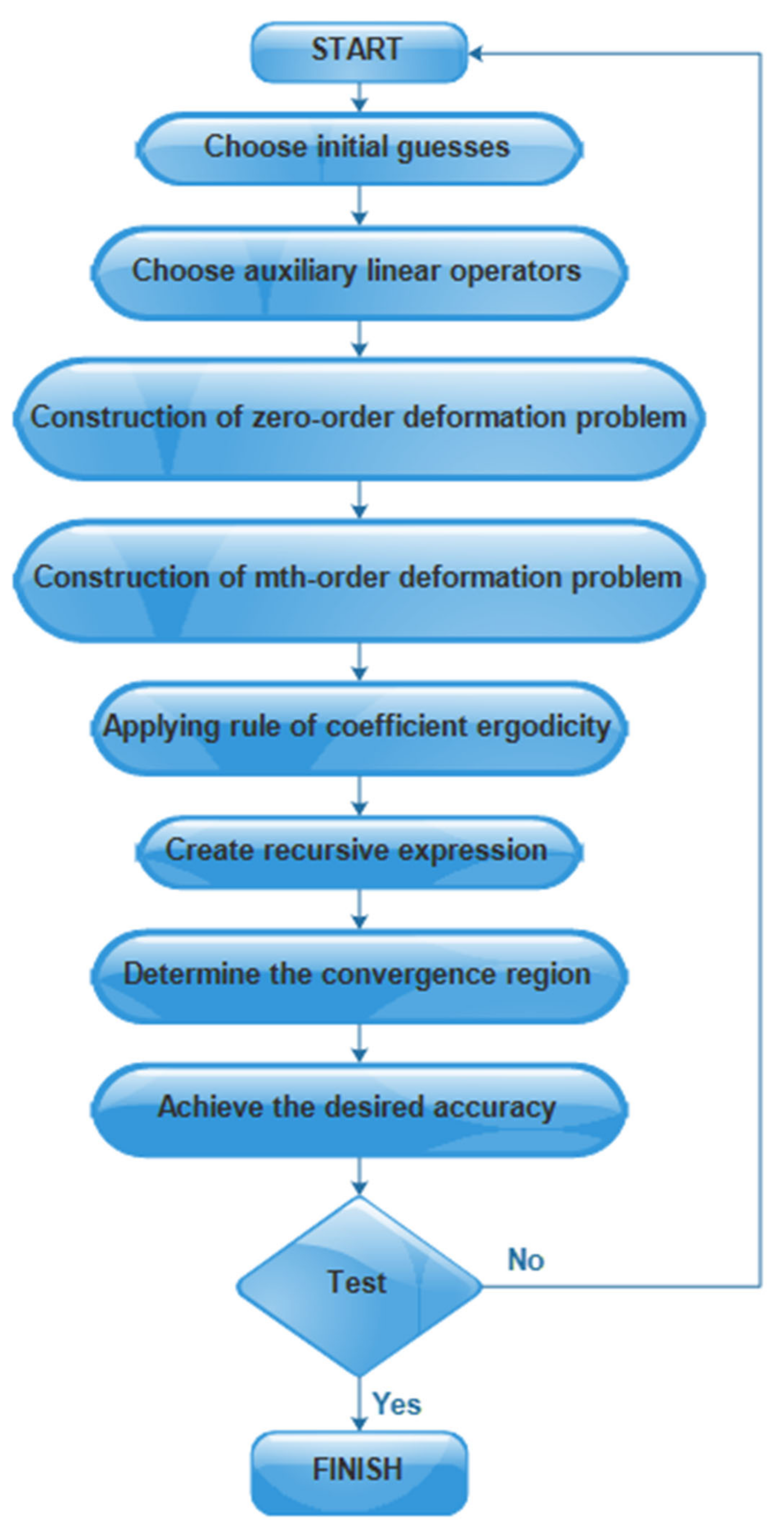
3. Homotopy Analysis Method

The set of dimensionless partial differential governing equations is very complex. Thus, the analytical solution of these equations is obtained by using the homotopy analysis method (HAM). The HAM method is one of the best semi-analytical methods that can be used to find solutions with excellent accuracy. This method, unlike the perturbation technique, does not impose any smaller parameter constraints. The flow chart of HAM method is presented in Figure 2. The method was proposed by Liao [31], and later, different studies are performed by using this method [32,33,34].

The initial guesses for the current flow problem are

$$\begin{array}{c}{f}_0(\xi ,\tau )=\sin \tau \left(1-\exp \left(-\xi \right)\right),\hspace{1em}{\theta }_0(\xi ,\tau )=\exp \left(-\xi \right),\hspace{1em}\hspace{1em}{\chi }_0(\xi ,\tau )=\exp \left(-\xi \right),\\ g_0(\xi ,\tau )=A\sin \tau \left(1-\exp \left(-\xi \right)\right),\hspace{1em}{\varphi }_0(\xi ,\tau )=\exp \left(-\xi \right).\end{array}\}$$

(20)

The linear auxiliary operators are

$$\begin{array}{ccccc}{\cancel{\cancel{\cancel{L}}}}_f=\frac{{\partial }^3}{\partial {\xi }^3}-\frac{\partial }{\partial \xi },& {\cancel{\cancel{\cancel{L}}}}_g=\frac{{\partial }^3}{\partial {\xi }^3}-\frac{\partial }{\partial \xi },& {\cancel{\cancel{\cancel{L}}}}_{\theta }=\frac{{\partial }^2}{\partial {\xi }^2}-1,& {\cancel{\cancel{\cancel{L}}}}_{\varphi }=\frac{{\partial }^2}{\partial {\xi }^2}-1,& {\cancel{\cancel{\cancel{L}}}}_{\chi }=\frac{{\partial }^2}{\partial {\xi }^2}-1.\end{array}$$

(21)

Fulfilling

$$\begin{array}{c}{\cancel{\cancel{\cancel{L}}}}_f\left({\displaystyle \sum _{k=0}^2{\cancel{\cancel{\cancel{\mathbb{Z}}}}}_{k+1}}{e}^{(k-1)\xi }\right)=0,\hspace{1em}{\cancel{\cancel{\cancel{L}}}}_g\left({\displaystyle \sum _{j=3}^5{\cancel{\cancel{\cancel{\mathbb{Z}}}}}_{k+1}}{e}^{(k-4)\xi }\right)=0,\hspace{1em}{\cancel{\cancel{\cancel{L}}}}_{\theta }\left({\displaystyle \sum _{j=6}^7{\cancel{\cancel{\cancel{\mathbb{Z}}}}}_{k+1}}{e}^{{(-1)}^k\xi }\right)=0,\\ {\cancel{\cancel{\cancel{L}}}}_{\varphi }\left({\displaystyle \sum _{k=8}^9{\cancel{\cancel{\cancel{\mathbb{Z}}}}}_{k+1}}{e}^{{(-1)}^k\xi }\right)=0,\hspace{1em}\hspace{1em}\hspace{1em}{\cancel{\cancel{\cancel{L}}}}_{\chi }\left({\displaystyle \sum _{k=10}^{11}{\cancel{\cancel{\cancel{\mathbb{Z}}}}}_{k+1}}{e}^{{(-1)}^k\xi }\right)=0,\end{array}\}$$

(22)

With ${\cancel{\cancel{\cancel{\mathbb{Z}}}}}_j\left(j=1,2,,\dots \dots .,12\right)$ being arbitrary constants. The analytic homotopic solution primarily depends on supplementary parameters $\left(h_{\varphi },h_{\theta },h_{\chi },h_f,h_g\right),$ and by giving accurate values to these parameters, the convergence can be reached. The region of convergence can be indicated by plotting $h-$ curve which is shown in Figure 3. The choice of auxiliary parameters should be feasible for $-1.2\le {\hslash }_f\le -0.2$, $-1.8\le {\hslash }_g\le -0.2$, $-1.3\le {\hslash }_{\theta }\le -0.2$, $-1\le {\hslash }_{\varphi }\le -0.05$, and $-1.2\le {\hslash }_{\chi }\le -0.4.$

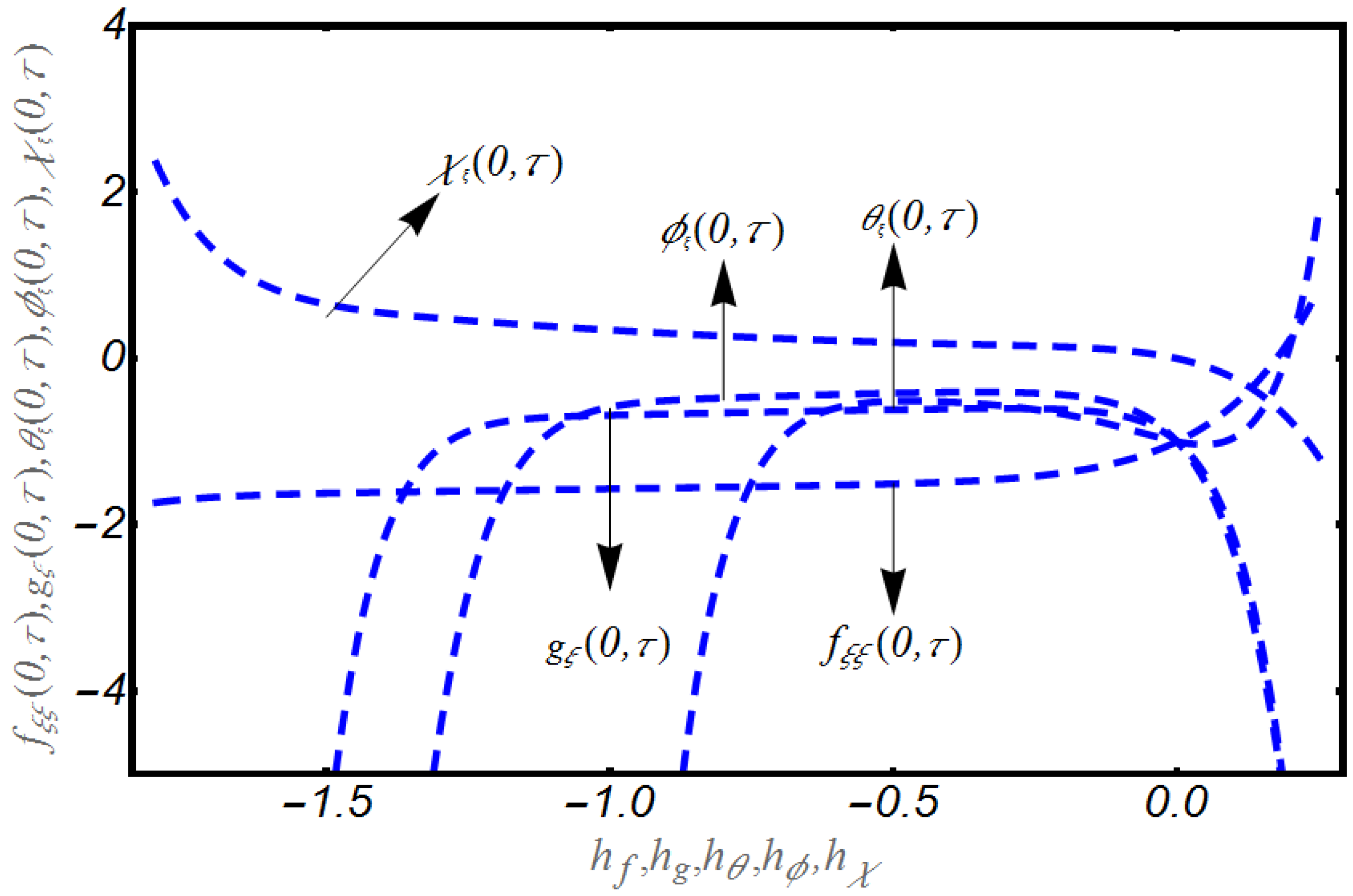
4. Verification of the Analytical Model

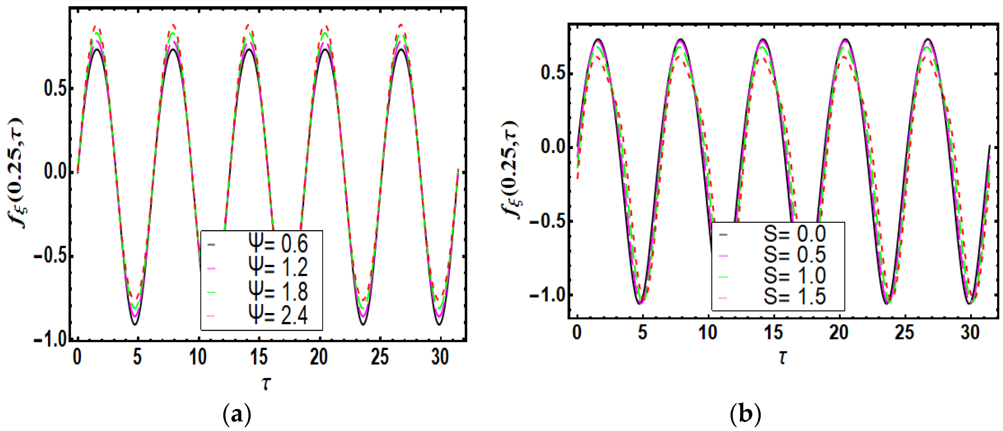
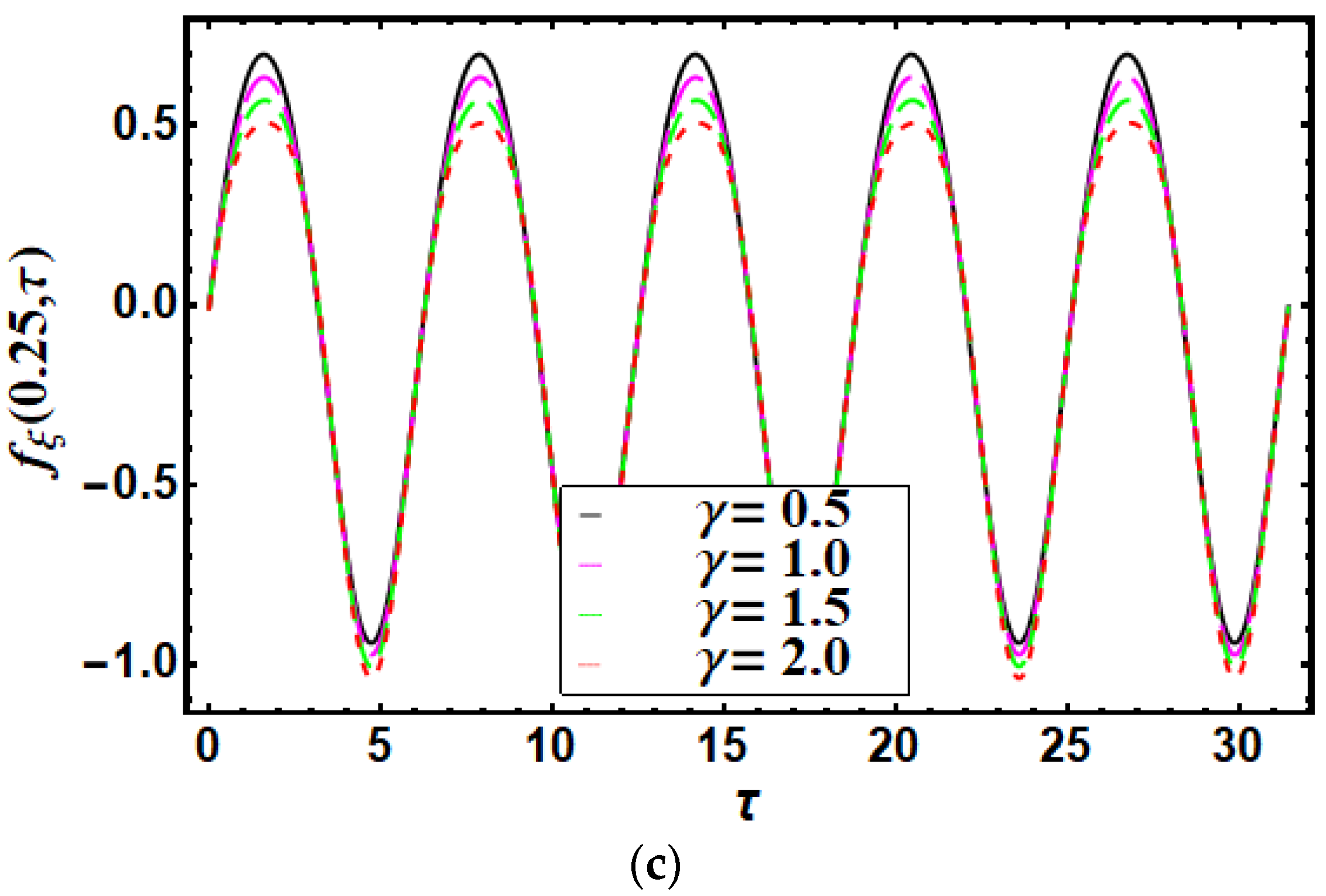
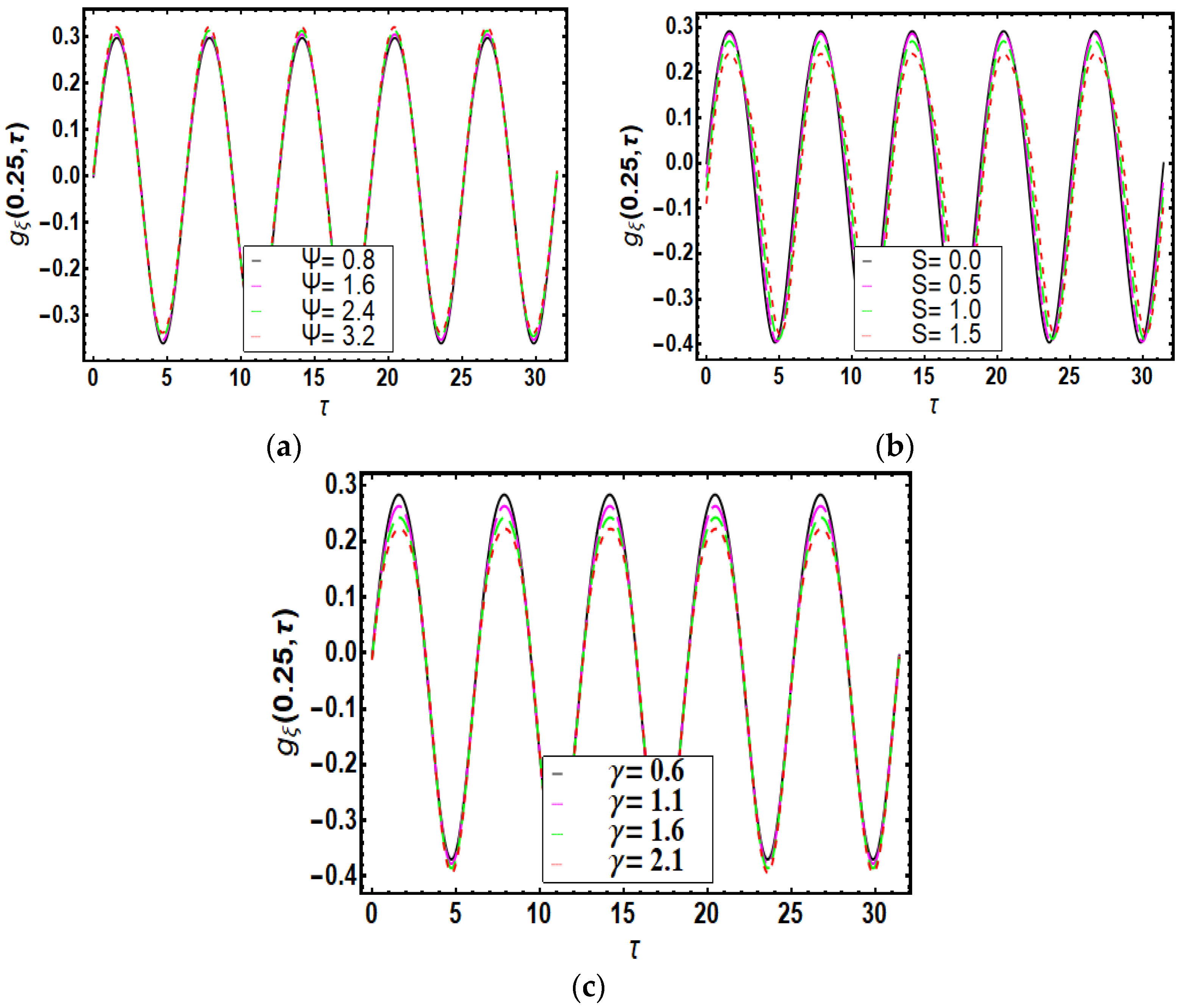
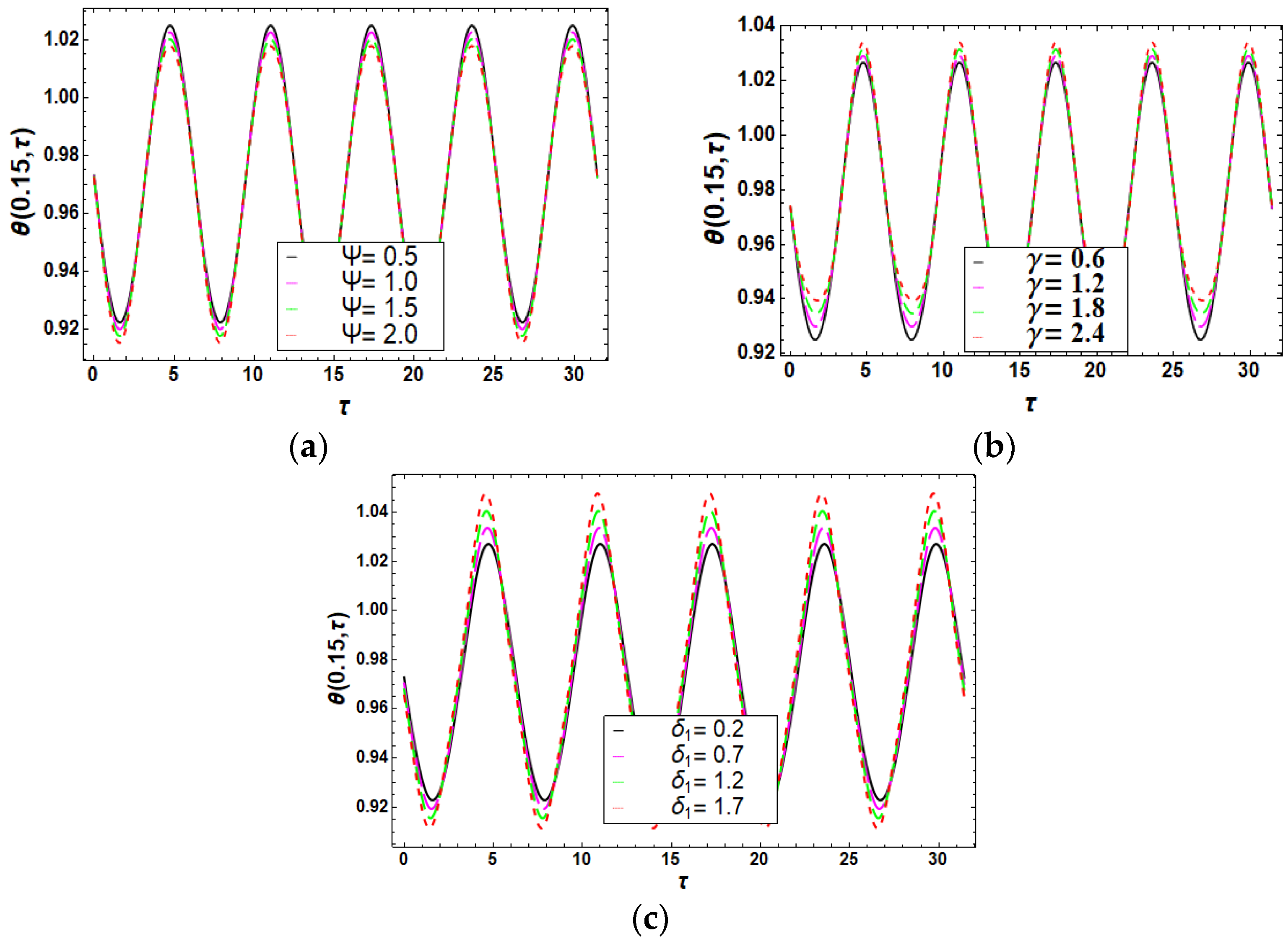
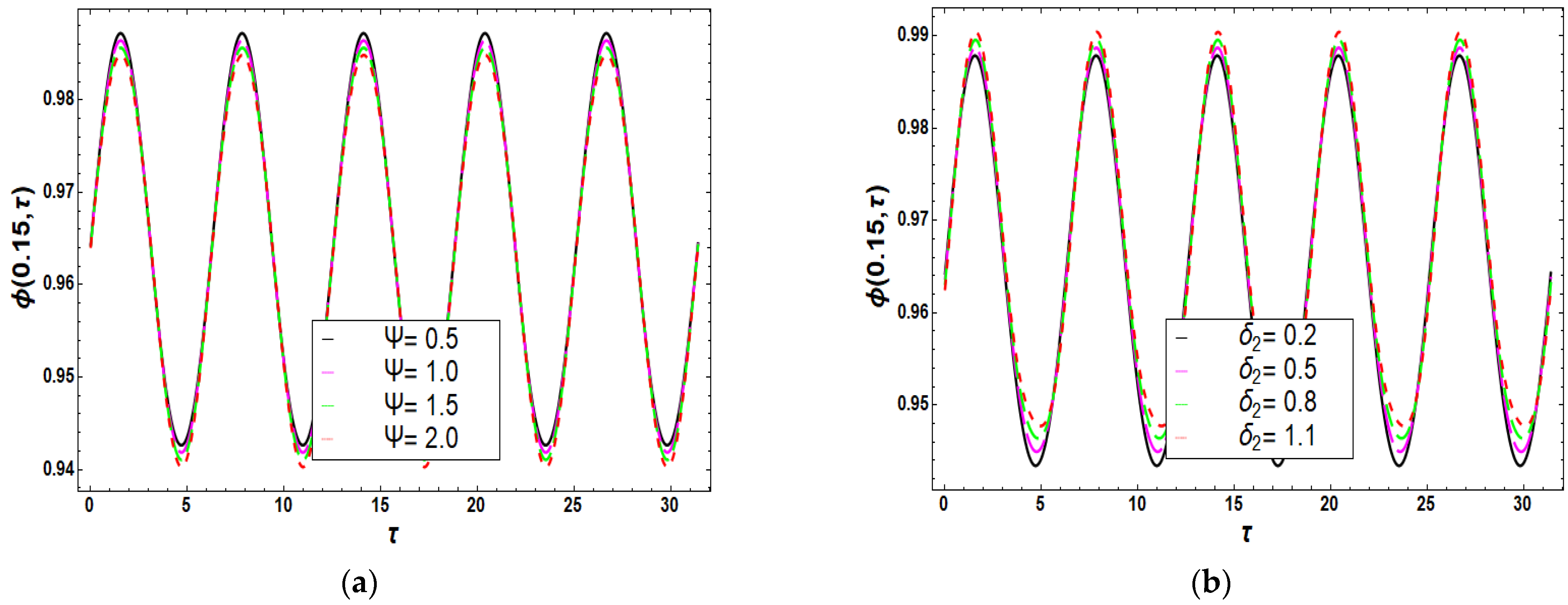
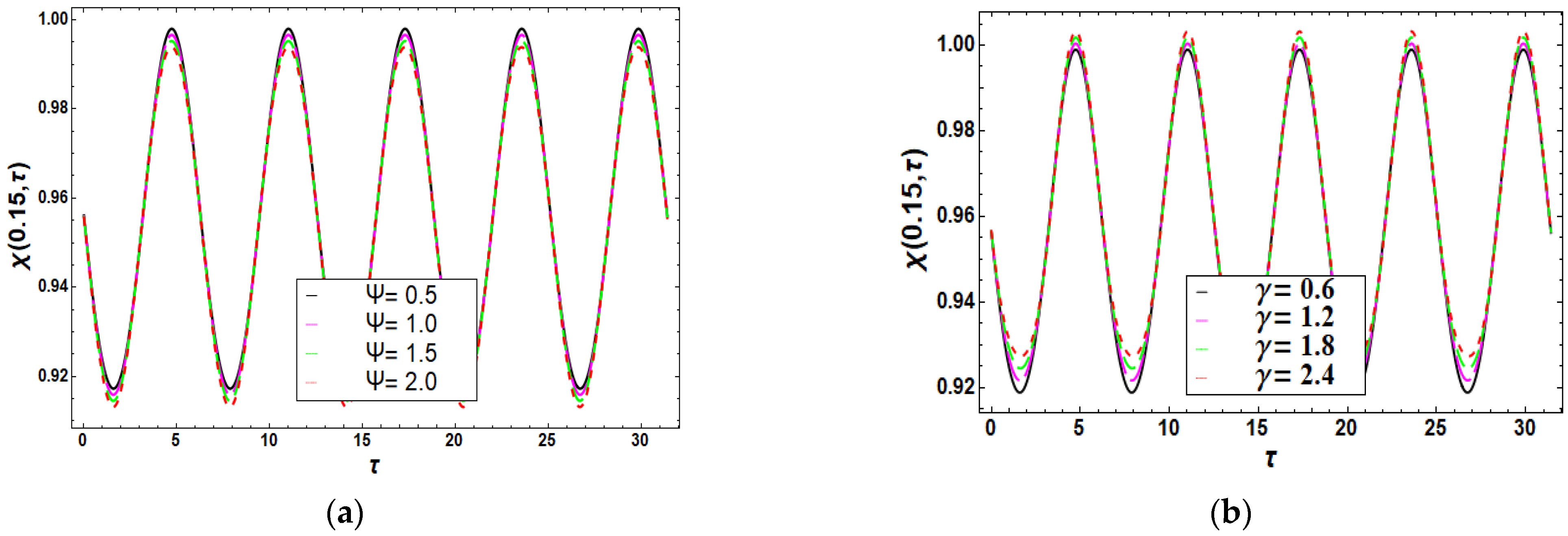
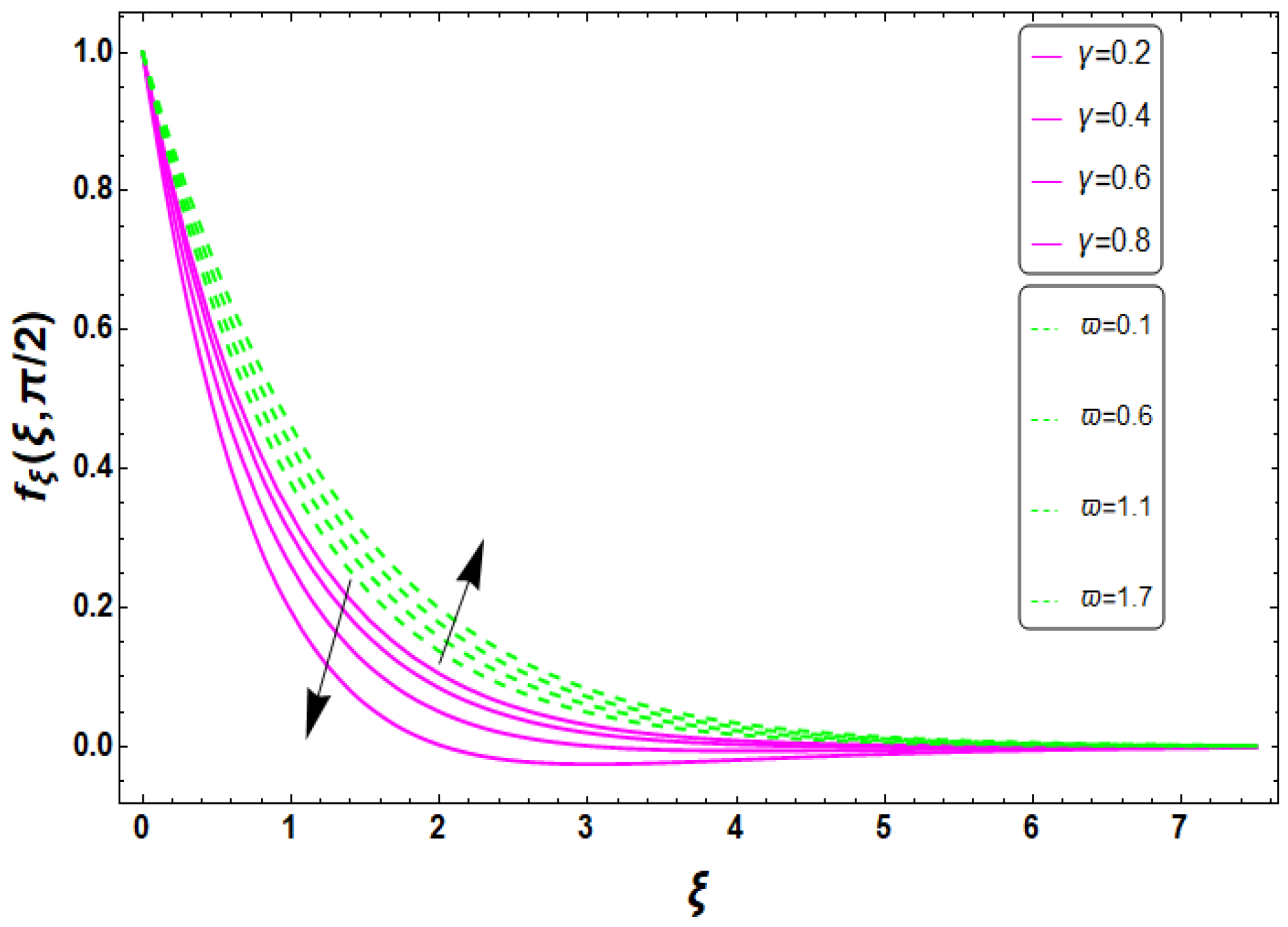
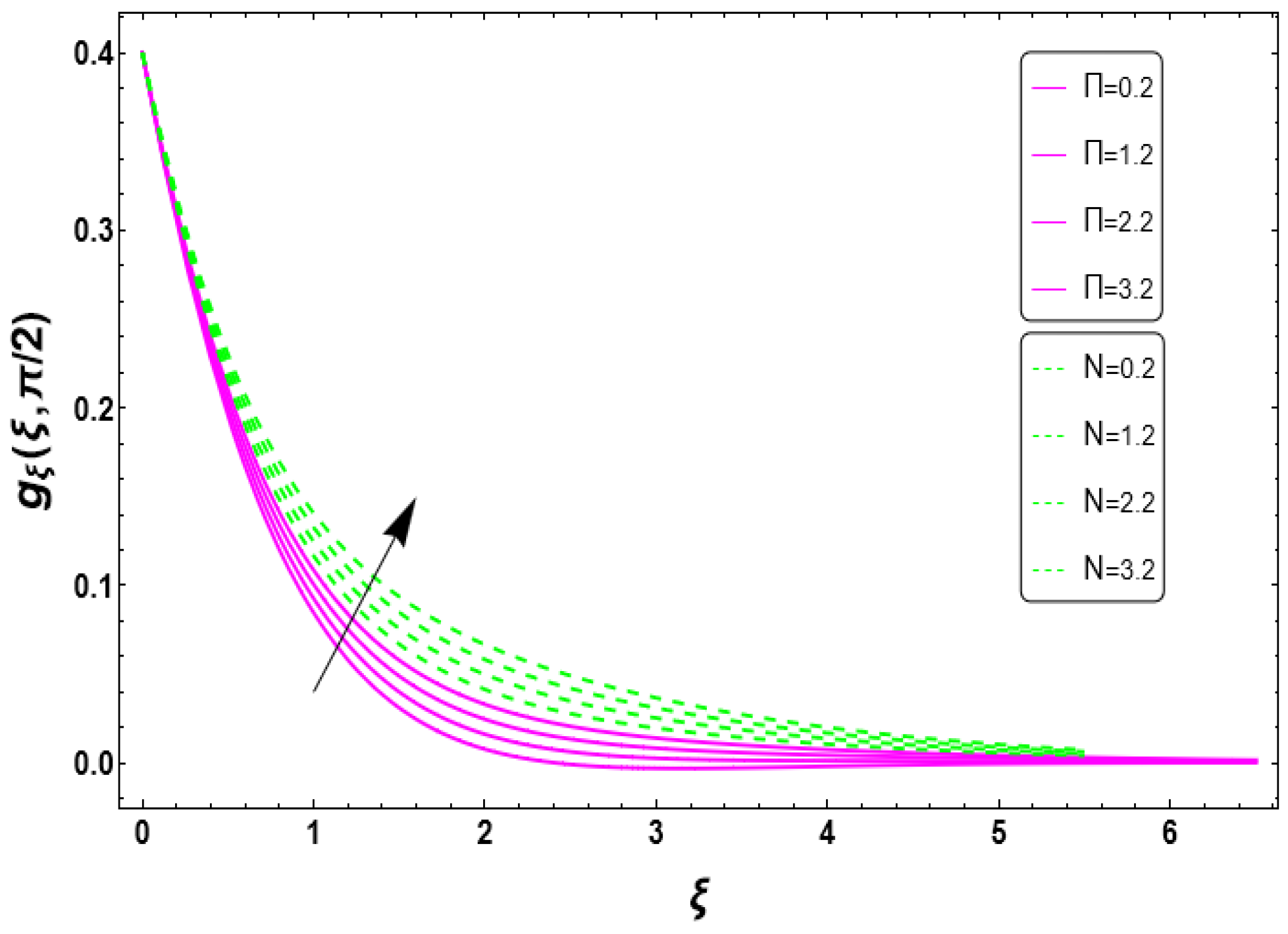
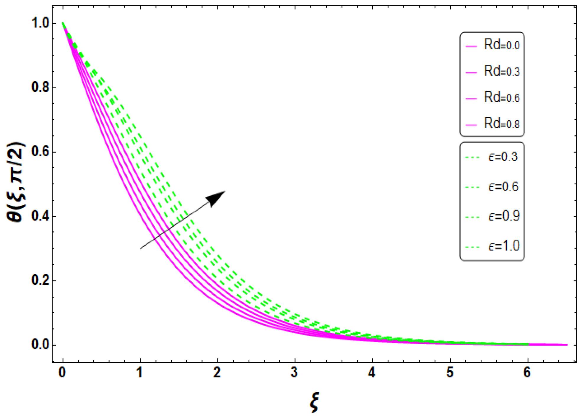
To check the validity of the current model, a comparison with the results of Ariel [27] is performed. As presented in

Table 1. Comparison of analytical findings with those of Ariel [35] for $S=\mathsf{\Omega }=\varpi =\mathsf{\Pi }=\gamma =0$.

	Ariel [35]		Present Results
$A$	$-f^{″}\left(0\right)$	$-g^{″}\left(0\right)$	$-f^{″}\left(0\right)$	$-g^{″}\left(0\right)$
0.0	1.00000	0.00000	1.00000	0.00000
0.1	1.02025	0.06684	1.020256	0.066856
0.2	1.03949	0.14873	1.039501	0.148719

, an excellent agreement between the results is encountered. It is to be mentioned that Ariel [35] studied the problem using the homotopy perturbation method.

5. Discussion

In this section, the velocity $\left(f_{\xi },g_{\xi }\right),$ temperature $\theta$, concentration $\varphi$, and microorganisms $\chi$ profiles are presented and discussed. The studied model is based on theoretical flow assumptions and the following parameters have been fixed as $\mathsf{\Omega }=0.2,$ $S=0.2,$ $\mathsf{\Psi }=0.4,$ ${\mathrm{N}}_{\mathrm{b}}=0.3,$ $\mathsf{\varpi }=0.2,$, ${\mathrm{N}}_{\mathrm{t}}=0.3$, $\mathrm{Pr}=2,$ $\mathsf{\Pi }=0.4,$ $\mathrm{N}=0.4,$ $\mathrm{Pr}=1.5,$ $\gamma =0.2,$ $\mathsf{\gamma }=0.5,$ ${\mathsf{\delta }}_1=0.1,$ $\epsilon =0.2$, $Sc=0.4,$ ${\mathsf{\delta }}_2=0.3,$ $\mathsf{\Delta }=0.3,$ $\mathsf{\Upsilon }=0.7,$ $\mathsf{\Lambda }=0.1,$ $\beta =0.7,$ $\mathsf{\Theta }=0.2,$ $\mathsf{\Gamma }=0.4$, and $m=\mathrm{0.4.}$ Figure 4a shows the effects of the Deborah number $\mathsf{\Psi }$ on the velocity field $f_{\xi }$. It is seen that the velocity $f_{\xi }$ obtains increasing variations for the rising values of $\mathsf{\Psi }.$ Physically, such observations are due to relaxation time features. Figure 4b is sketched to represent the behavior of $f_{\xi }$ against different impacts of the oscillating frequency to the stretching rate $S$. The increasing of $S$ causes a reduction in $f_{\xi }$. Moreover, a minor phase shift is also noticed for higher values of $S.$ Figure 4c presents the effects of the porosity parameter $\gamma$ on $f_{\xi }$. A decrease in the velocity oscillations occurs when $\gamma$ is increased. Such observations are physically associated to the permeability of the porous media.

Figure 5a is plotted to analyze the effect of $\mathsf{\Psi }$ on the velocity profile $g_{\xi }$. An increase in the oscillation amplitude of the velocity is encountered when $\mathsf{\Psi }$ is increased. Figure 5b depicts the variation in the velocity $g_{\xi }$ for different values of $S.$ A reducing nature of the velocity is observed when larger $S$ values are imposed. Such observations are associated to the oscillating frequency. Figure 5c is drawn to describe the behavior of $g_{\xi }$ for various values of $\gamma$. A declining trend of the velocity amplitude is noticed when $\gamma$ is increased. Such declining behavior is due to the permeability of porous media.

Figure 6a describes the temporal variations in the temperature for various values of $\mathsf{\Psi }.$ The temperature $\theta$ decreases with an increasing value of $\mathsf{\Psi }.$ Figure 6b presents the temperature variations for different values of the permeability parameter $\gamma$. The increase in $\gamma$ leads to an augmentation of the temperature. Figure 6c is plotted to demonstrate the behavior of the temperature profile $\theta$ when the thermic relaxation constant ${\mathsf{\delta }}_1$ is varied. A considerable increase in the temperature occurs for higher values of ${\mathsf{\delta }}_1$.

Figure 7a shows the influence of $\mathsf{\Psi }$ on the concentration profile $\varphi$. A reduction in the concentration amplitude occurs when $\mathsf{\Psi }$ is increased. Figure 7b presents the concentration variations $\varphi$ for different solutal relaxation ${\mathsf{\delta }}_2$ values. It is shown that the increase in ${\mathsf{\delta }}_2$ causes an increase in the concentration. Figure 8a shows the variation in the motile microorganisms $\chi$ for various $\mathsf{\Psi }$ (Deborah number) values. It is noticed that the increase in $\mathsf{\Psi }$ causes the increase in the motile microorganisms’ values. Figure 8b presents the behavior of the motile microorganisms $\chi$ for different values of $\gamma$. It is seen that the motile microorganisms are higher for higher values of $\gamma$.

Figure 9 presents the velocity profile $f_{\xi }$ for various porosity parameter $\gamma$ and mixed convection parameter $\varpi$. It is noticed that the velocity increases with $\varpi$, while the opposite occurs for $\gamma .$ Figure 10 is sketched to show the profile of $g_{\xi }$ for different values of the bioconvective Rayleigh number $\mathsf{\Pi }$ and buoyancy ratio $N$. The increases in the Rayleigh number and buoyancy ratio lead to the intensification of the flow due to the density variation and thus cause the increase in the velocity.

Figure 11 depicts the impact of the radiation parameter $Rd$ and thermal conductivity parameter $\epsilon$ on the temperature profile $\theta .$ Both of these parameters have a beneficial effect of the temperature increasing. The augmentation of the temperature due to $Rd$ is associated to the electromagnetic waves. The thermal radiation effects are important in enhancing the heat transfer rate and have several applications in solar management systems. The increase in the thermal conductivity leads to an enhancement of the heat transfer rate and consequently an increase in the temperature. In Figure 12, the observations are predicted for $\theta$ due to the Brownian motion parameter $N_b$ and the ratio of the oscillating frequency to the stretched rate $S.$ A larger thermal contribution of $\theta$ for larger $N_b$ is exhibited. Physically, the increasing heat transfer rate is due to the random motion of tiny particles. The enhancement in $\theta$ for $S$ is due to a larger oscillating frequency.

Figure 13 is plotted to depict the profiles of $\varphi$ for different values of the thermophoresis parameter $N_t$ and activation energy factor $\mathsf{\Theta }$. An improvement in the concentration profile is noticed due to the increase in $N_t$ and $\mathsf{\Theta }$. The thermophoresis phenomenon is caused by the motions of the tiny particles from the hot region toward the cold surface. This migration reveals an enhancement in the concentration pattern of the tiny particles. Due to the intensification of the chemical process, the increase in concentration occurs also when the activation energy parameter is increased. Figure 14 demonstrates the behavior of the concentration profile $\varphi$ caused by the variation in the reaction rate $\mathsf{\Delta }$ and temperature difference parameter $\mathsf{\Lambda }$ values. It can be concluded that for larger $\mathsf{\Delta }$ and $\mathsf{\Lambda }$ values, a decrease in concentration $\varphi$ is noticed. Figure 15 presents the variations in $\varphi$ for different values of the Schmidt number $Sc$ and solutal relaxation ${\delta }_2$. Lower values of $\varphi$ are encountered with the increase in $Sc$. Physically, such observations are due to the smaller mass diffusivities. Similar observations can be mentioned for the effect of solutal relaxation ${\delta }_2$. Figure 16 shows the motile microorganisms’ profiles $\chi$ for various values of $\beta$ (bioconvective Peclet number) and $\mathsf{\Upsilon }$ (bioconvective Lewis number). It is clear that when the values of $\beta$ and $\mathsf{\Upsilon }$ increase, they cause a reduction in the motile microorganisms’ values $\chi$. Figure 17 shows the profiles of $\chi$ for different values of the Peclet $Pe$ and bioconvective Lewis numbers $Lb$. A reduction in $\chi$ is noticed for lower $Pe$ and $Lb$ values. This reduction is associated to the low motile densities. Figure 18 is plotted to show the behavior of motile microorganisms caused by the change in the $\mathsf{\Gamma }$ (concentration difference constant for microorganisms) and $\gamma$ (porosity parameter) values. The microorganism’s concentration is enhanced with higher $\mathsf{\Gamma }$ values but decreases with $\gamma$.

Table 2. Physical implications of parameters for $N{u}_{\tilde{x}}{\left({\mathrm{Re}}_{\tilde{x}}\right)}^{-0.5}$, $S{h}_{\tilde{x}}{\left({\mathrm{Re}}_{\tilde{x}}\right)}^{-0.5}$, and $N{n}_{\tilde{x}}{\left({\mathrm{Re}}_{\tilde{x}}\right)}^{-0.5}$.

$\mathsf{\Omega }$	$\mathsf{\Psi }$	$\mathbf{Pr}$	${\mathsf{\delta }}_1$	$\mathit{\epsilon }$	$\mathit{\gamma }$	$\mathit{N}{\mathit{u}}_{\tilde{\mathit{x}}}{\left({\mathbf{Re}}_{\tilde{\mathit{x}}}\right)}^{-0.5}$	$\mathit{S}{\mathit{h}}_{\tilde{\mathit{x}}}{\left({\mathbf{Re}}_{\tilde{\mathit{x}}}\right)}^{-0.5}$	$\mathit{N}{\mathit{n}}_{\tilde{\mathit{x}}}{\left({\mathbf{Re}}_{\tilde{\mathit{x}}}\right)}^{-0.5}$
0.4	0.2	1.5	0.3	0.2	0.4	0.5562	0.41537	0.5394
0.5						0.5342	0.3857	0.5246
0.6						0.5279	0.3646	0.4942
0.2	0.50					0.4404	0.38325	0.5131
						0.4724	0.3956	0.4823
						0.4968	0.43577	0.4634
		0.7				0.4505	0.4156	0.5332
		1.1				0.4877	0.43435	0.5554
		1.5				0.5143	0.4435	0.5635
			0.2			0.4403	0.45032	0.5642
			0.3			0.4654	0.46435	0.5847
			0.4			0.5153	0.4935	0.6242
				0.3		0.4345	0.40466	0.5035
				0.5		0.3965	0.38466	0.4842
				0.7		0.3546	0.37343	0.4435
					0.4	0.4832	0.49353	0.55456
					0.6	0.4353	0.43577	0.5246
					0.8	0.3868	0.41334	0.4756

presents the computed outcomes of $N{u}_{\tilde{x}}{\left({\mathrm{Re}}_{\tilde{x}}\right)}^{-0.5}$, $S{h}_{\tilde{x}}{\left({\mathrm{Re}}_{\tilde{x}}\right)}^{-0.5}$, and $N{n}_{\tilde{x}}{\left({\mathrm{Re}}_{\tilde{x}}\right)}^{-0.5}$ for several values of the governing parameters. Smaller values of these physical quantities occur for higher values of $\mathsf{\Omega }$, $\gamma$, and $\epsilon .$

6. Conclusions

The bioconvective Jeffrey fluid conveying tiny particles with variable thermal conductivity is studied. The mass and heat transfers are modeled using Cattaneo–Christov diffusion theories. The bidirectional porous oscillating surface induces the flow. The dimensionless system is solved via the homotopy analysis scheme. The convergence of the HAM scheme is ensured. The main findings can be summarized as follows:

• An increase in the amplitude of the velocity occurs for a higher Deborah number without any phase shift.
• A lower velocity magnitude is encountered for the porosity parameter.
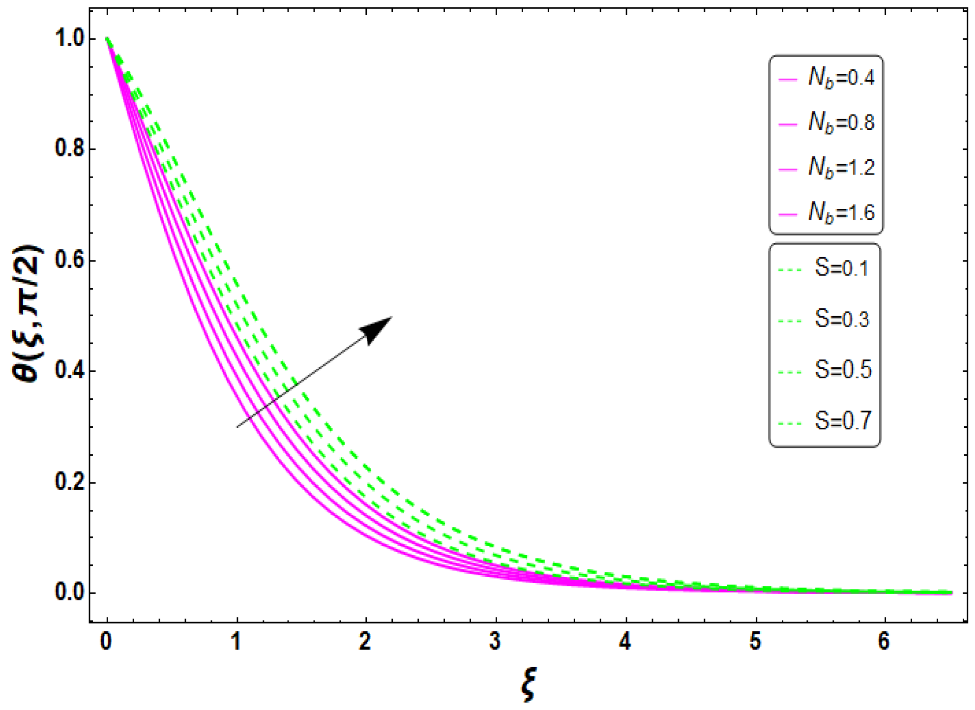
• The temporal variation in the temperature time increases with the increase in the thermic relaxation constant and the porosity parameter.
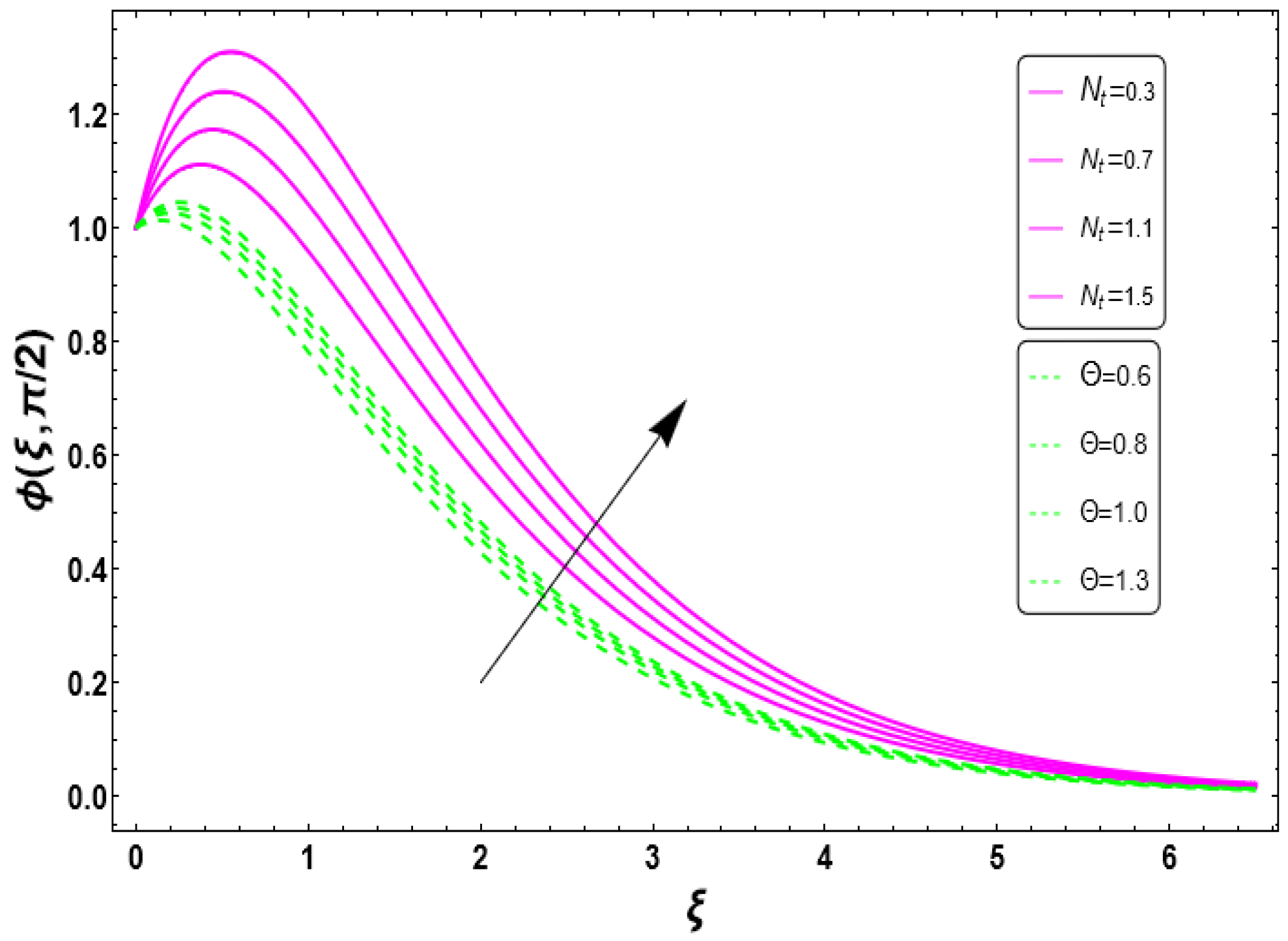
• The impact of the Deborah number has been found to reduce the concentration and microorganisms’ profiles.
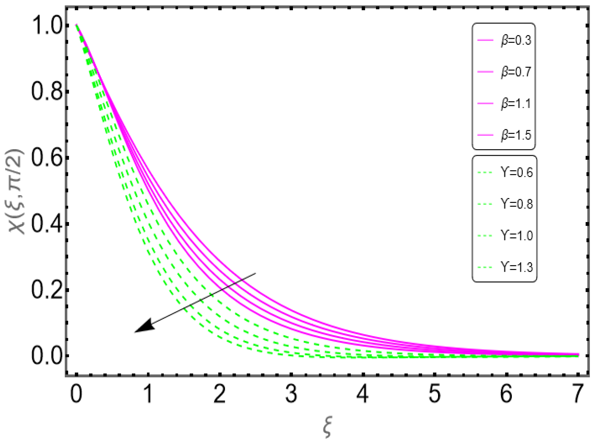
• The temperature profiles have higher values for a higher radiation parameter and the ratio of the oscillating frequency to the stretched rate.
• The variable thermal conductivity assumptions are very effective in improving the heat transfer rate.
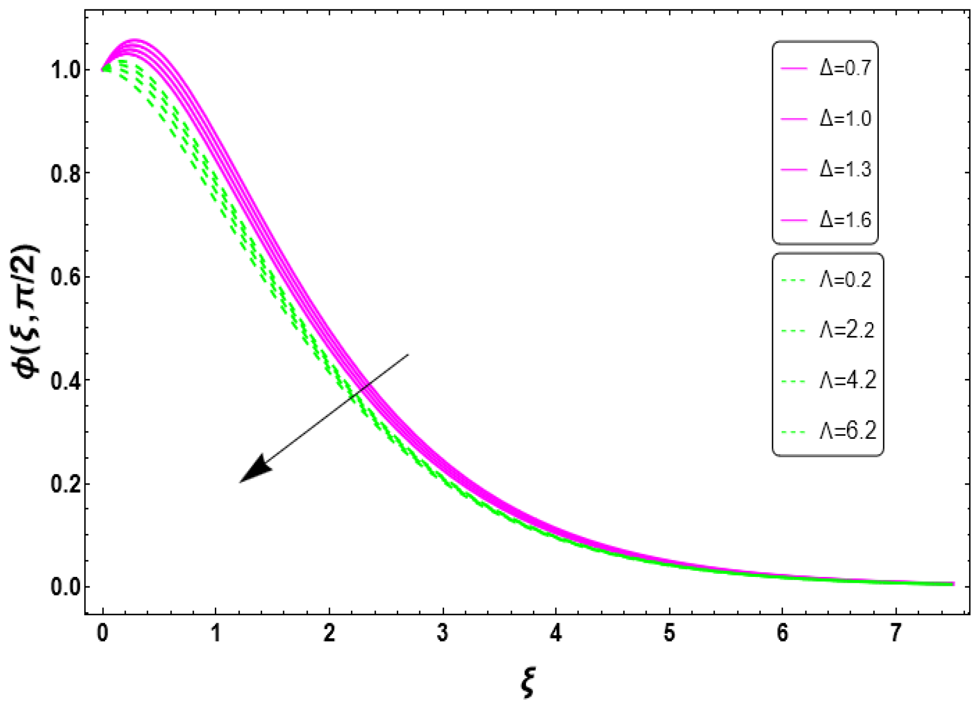
• The increase in the chemical reaction parameter, Lewis number, and solutal relaxation reduces the concentration profile.
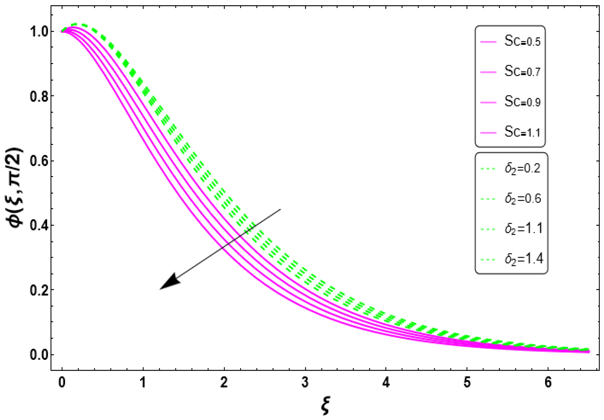
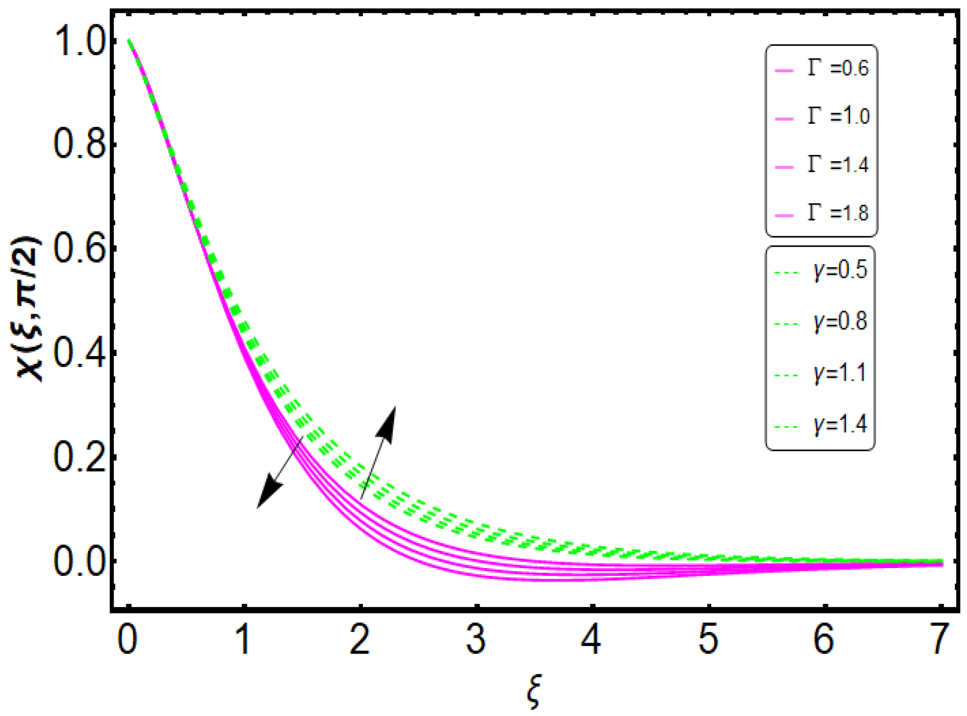
• With the increment of the concentration difference constant, the microorganism profile has lower values.
• With an increasing porosity parameter, the microorganism profile is enhanced.
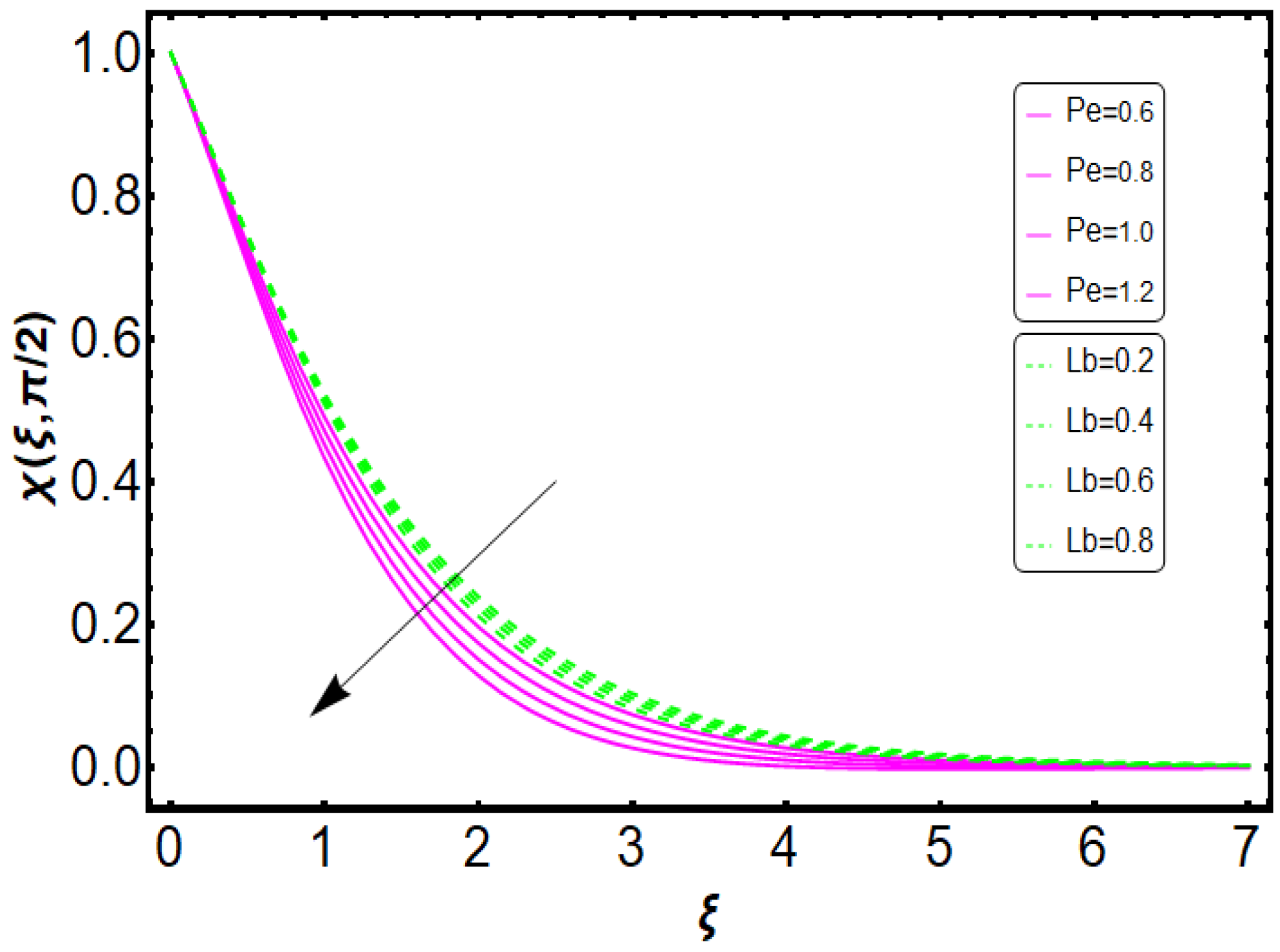
• The Local Nusselt number, Sherwood number, and motile density number are enhanced with the Prandtl number and thermic relaxation constant.

References

1. Choi, S.U.S. Enhancing thermal conductivity of fluids with nanoparticles. ASME-Publ. Fed. 1995, 231, 99–106. [Google Scholar]
2. Buongiorno, J. Convective transport in nanofluids. J. Heat Transf. 2006, 128, 240–250. [Google Scholar] [CrossRef]
3. Mahmud, K.; Rana, S.; Al-Zubaidi, A.; Mehmood, R.; Saleem, S. Interaction of Lorentz force with cross swimming microbes in couple stress nano fluid past a porous Riga plate. Int. Commun. Heat Mass Transf. 2022, 138, 106347. [Google Scholar] [CrossRef]
4. Madkhali, H.A.; Haneef, M.; El-Shafay, A.S.; Alharbi, S.O.; Nawaz, M. Mixed convective transport in Maxwell hybrid nano-fluid under generalized Fourier and Fick laws. Int. Commun. Heat Mass Transf. 2022, 130, 105714. [Google Scholar] [CrossRef]
5. Hameed, N.; Noeiaghdam, S.; Khan, W.; Pimpunchat, B.; Fernandez-Gamiz, U.; Khan, M.S.; Rehman, A. Analytical analysis of the magnetic field, heat generation and absorption, viscous dissipation on couple stress casson hybrid nano fluid over a nonlinear stretching surface. Results Eng. 2022, 16, 100601. [Google Scholar] [CrossRef]
6. Chandrasekaran, M.; Prakash, K.B.; Subramaniyan, C.; Santhosh, N.; Tamilarasan, V.D. Experimental investigation on heavy duty engine radiator using cerium oxide nano fluid. Mater. Today Proc. 2022, 66, 1497–1500. [Google Scholar] [CrossRef]
7. Cui, J.; Razzaq, R.; Farooq, U.; Khan, W.A.; Farooq, F.B.; Muhammad, T. Impact of non-similar modeling for forced convection analysis of nano-fluid flow over stretching sheet with chemical reaction and heat generation. Alex. Eng. J. 2022, 61, 4253–4261. [Google Scholar] [CrossRef]
8. Mishra, G.; Chhabra, R.P. Effects of flow fluctuations and buoyancy on heat transfer from a sphere in non-Newtonian nano fluids: Potential for intensification. Chem. Eng. Process. Process Intensif. 2022, 178, 109048. [Google Scholar] [CrossRef]
9. Mahmud, K.; Mehmood, R.; Rana, S.; Al-Zubaidi, A. Flow of magnetic shear thinning nano fluid under zero mass flux and hall current. J. Mol. Liq. 2022, 352, 118732. [Google Scholar] [CrossRef]
10. Balaji, T.; Rajendiran, S.; Selvam, C.; Lal, D.M. Enhanced heat transfer characteristics of water based hybrid nanofluids with graphene nanoplatelets and multi walled carbon nanotubes. Powder Technol. 2021, 394, 1141–1157. [Google Scholar] [CrossRef]
11. Manohar, G.R.; Venkatesh, P.; Gireesha, B.J.; Madhukesh, J.K.; Ramesh, G.K. Dynamics of hybrid nanofluid through a semi spherical porous fin with internal heat generation. Partial. Differ. Equ. Appl. Math. 2021, 4, 100150. [Google Scholar] [CrossRef]
12. Chen, Y.; Luo, P.; Tao, Q.; Liu, X.; He, D. Natural convective heat transfer investigation of nanofluids affected by electrical field with periodically changed direction. Int. Commun. Heat Mass Transf. 2021, 128, 105613. [Google Scholar] [CrossRef]
13. Jaafar, A.; Jamaludin, A.; Nasir, N.A.A.M.; Nazar, R.; Pop, I. MHD opposing flow of Cu−TiO2 hybrid nanofluid under an exponentially stretching/shrinking surface embedded in porous media with heat source and slip impacts. Results Eng. 2023, 17, 101005. [Google Scholar] [CrossRef]
14. Mustafa, J.; Abdullah, M.M.; Ahmad, M.Z.; Husain, S.; Sharifpur, M. Numerical study of two-phase turbulence nanofluid flow in a circular heatsink for cooling LEDs by changing their location and dimensions. Eng. Anal. Bound. Elem. 2023, 149, 248–260. [Google Scholar] [CrossRef]
15. Zainal, N.A.; Waini, I.; Khashi’ie, N.S.; Kasim, A.R.M.; Naganthran, K.; Nazar, R.; Pop, I. Stagnation point hybrid nanofluid flow past a stretching/shrinking sheet driven by Arrhenius kinetics and radiation effect. Alex. Eng. J. 2023, 68, 29–38. [Google Scholar] [CrossRef]
16. Abdollahi, S.A.; Alizadeh, A.A.; Esfahani, i.C.; Zarinfar, M.; Pasha, P. Investigating heat transfer and fluid flow betwixt parallel surfaces under the influence of hybrid nanofluid suction and injection with numerical analytical technique. Alex. Eng. J. 2023, 70, 423–439. [Google Scholar] [CrossRef]
17. Shahzad, A.; Imran, M.; Tahir, M.; Khan, S.A.; Akgül, A.; Abdullaev, S.; Park, C.; Zahran, H.Y.; Yahia, I.S. Brownian motion and thermophoretic diffusion impact on Darcy-Forchheimer flow of bioconvective micropolar nanofluid between double disks with Cattaneo-Christov heat flux. Alex. Eng. J. 2023, 62, 1–15. [Google Scholar] [CrossRef]
18. Kairi, R.R.; Roy, S.; Raut, S. Stratified thermosolutal Marangoni bioconvective flow of gyrotactic microorganisms in Williamson nanofluid. Eur. J. Mech. B/Fluids 2023, 97, 40–52. [Google Scholar] [CrossRef]
19. Hussain, S.; Aly, A.M.; Alsedias, N. Bioconvection of oxytactic microorganisms with nano-encapsulated phase change materials in an omega-shaped porous enclosure. J. Energy Storage 2022, 56, 105872. [Google Scholar] [CrossRef]
20. Din, I.S.U.; Siddique, I.; Ali, R.; Jarad, F.; Abdal, S.; Hussain, S. On heat and flow characteristics of Carreau nanofluid and tangent hyperbolic nanofluid across a wedge with slip effects and bioconvection. Case Stud. Therm. Eng. 2022, 39, 102390. [Google Scholar] [CrossRef]
21. Mariam, A.; Siddique, I.; Abdal, S.; Jarad, F.; Ali, R.; Salamat, N.; Hussain, S. Bioconvection attribution for effective thermal transportation of upper convicted Maxwell nanofluid flow due to an extending cylindrical surface. Case Stud. Therm. Eng. 2022, 34, 102062. [Google Scholar] [CrossRef]
22. Cui, J.; Munir, S.; Raies, S.F.; Farooq, U.; Razzaq, R. Non-similar aspects of heat generation in bioconvection from flat surface subjected to chemically reactive stagnation point flow of Oldroyd-B fluid. Alex. Eng. J. 2022, 61, 5397–5411. [Google Scholar] [CrossRef]
23. Habib, D.; Abdal, S.; Ali, R.; Baleanu, D.; Siddique, I. On bioconvection and mass transpiration of micropolar nanofluid dynamics due to an extending surface in existence of thermal radiations. Case Stud. Therm. Eng. 2021, 27, 101239. [Google Scholar] [CrossRef]
24. Waqas, H.; Naseem, R.; Muhammad, T.; Farooq, U. Bioconvection flow of Casson nanofluid by rotating disk with motile microorganisms. J. Mater. Res. Technol. 2021, 13, 2392–2407. [Google Scholar] [CrossRef]
25. Baranovskii, E.S. Flows of a polymer fluid in domain with impermeable boundaries. Comput. Math. Math. Phys. 2014, 54, 1589–1596. [Google Scholar] [CrossRef]
26. Muzara, H.; Shateyi, S. MHD Laminar Boundary Layer Flow of a Jeffrey Fluid Past a Vertical Plate Influenced by Viscous Dissipation and a Heat Source/Sink. Mathematics 2021, 9, 1896. [Google Scholar] [CrossRef]
27. Raje, A.; Bhise, A.A.; Kulkarni, A. Entropy analysis of the MHD Jeffrey fluid flow in an inclined porous pipe with convective boundaries. Int. J. Therm. 2023, 17, 100275. [Google Scholar] [CrossRef]
28. Khan, Z.A.; Shah, N.A.; Haider, N.; El-Zahar, E.R.; Yook, S.J. Analysis of natural convection flows of Jeffrey fluid with Prabhakar-like thermal transport. Case Stud. Therm. Eng. 2022, 35, 102079. [Google Scholar] [CrossRef]
29. Nabwey, H.A.; Mushtaq, M.; Nadeem, M.; Ashraf, M.; Rashad, A.M.; Alshber, S.I.; Hawsah, M.A. Note on the Numerical Solutions of Unsteady Flow and Heat Transfer of Jeffrey Fluid Past Stretching Sheet with Soret and Dufour Effects. Mathematics 2022, 10, 4634. [Google Scholar] [CrossRef]
30. Ahmad, I.; Aziz, S.; Ali, N.; Khan, S.U. Radiative unsteady hydromagnetic 3D flow model for Jeffrey nanofluid configured by an accelerated surface with chemical reaction. Heat Transf. Asian Res. 2021, 50, 942–966. [Google Scholar] [CrossRef]
31. Liao, S.J. On the Analytic Solution of Magnetohydrodynamic Flows of non-Newtonian Fluids over a stretching sheet. J. Fluid Mech. 2003, 488, 189–212. [Google Scholar] [CrossRef] [Green Version]
32. Turkyilmazoglu, M. Numerical and Analytical solutions for the Flow and Heat Transfer near the Equator of an MHD Boundary layer over a Porous Rotating sphere. Int. J. Therm. Sci. 2011, 50, 831–842. [Google Scholar] [CrossRef]
33. Abbasbandy, S.; Shirzadi, A. Homotopy Analysis Method for a Nonlinear Chemistry Problem. Stud. Nonlinear Sci. 2010, 1, 127–132. [Google Scholar]
34. Dinarvand, S.; Abbassi, A.; Hosseini, R.; Pop, I. Homotopy analysis method for mixed convective boundary layer flow of a nanofluid over a vertical circular cylinder. Therm. Sci. 2015, 19, 549–561. [Google Scholar] [CrossRef]
35. Ariel, P.D. The three-dimensional flow past a stretching sheet and the homotopy perturbation method. Comput. Math. Appl. 2007, 54, 920–925. [Google Scholar] [CrossRef] [Green Version]
Figure 1. Flow geometry of the problem.
Mathematics 11 01600 g001
Figure 2. Flow chart of HAM method.
Mathematics 11 01600 g002
Figure 3. Curves for f , θ , ϕ , and χ .
Mathematics 11 01600 g003
Figure 4. (a) Effects of Ψ on f ξ . (b) Effects of S on f ξ . (c) Effects of γ on f ξ .
Mathematics 11 01600 g004aMathematics 11 01600 g004b
Figure 5. (a) Effects of Ψ on g ξ . (b) Effects of S on g ξ . (c) Effects of γ on g ξ .
Mathematics 11 01600 g005
Figure 6. (a) Effects of Ψ on θ . (b) Effects of γ on θ . (c) Effects of δ 1 on θ .
Mathematics 11 01600 g006
Figure 7. (a) Effects of Ψ on ϕ . (b) Effects of δ 2 on ϕ .
Mathematics 11 01600 g007
Figure 8. (a) Effects of ψ on χ . (b) Effects of γ on χ .
Mathematics 11 01600 g008
Figure 9. Profile of f ξ for various values of γ and ϖ .
Mathematics 11 01600 g009
Figure 10. Profile of g ξ for various values Π and N .
Mathematics 11 01600 g010
Figure 11. Profile of θ for various values of R d and ε .
Mathematics 11 01600 g011
Figure 12. Profile of θ for various values of N b and S .
Mathematics 11 01600 g012
Figure 13. Profile of ϕ for N t and Θ .
Mathematics 11 01600 g013
Figure 14. Profile of ϕ for Δ and Λ .
Mathematics 11 01600 g014
Figure 15. Profile of ϕ for S c and δ 2 .
Mathematics 11 01600 g015
Figure 16. Profile of χ for β and ϒ .
Mathematics 11 01600 g016
Figure 17. Profile of χ for P e and L b .
Mathematics 11 01600 g017
Figure 18. Profile of χ for Γ and γ .
Mathematics 11 01600 g018