A Fresnel Cosine Integral WASD Neural Network for the Classification of Employee Attrition

Abstract

Employee attrition, defined as the voluntary resignation of a subset of a company’s workforce, represents a direct threat to the financial health and overall prosperity of a firm. From lost reputation and sales to the undermining of the company’s long-term strategy and corporate secrets, the effects of employee attrition are multidimensional and, in the absence of thorough planning, may endanger the very existence of the firm. It is thus impeccable in today’s competitive environment that a company acquires tools that enable timely prediction of employee attrition and thus leave room either for retention campaigns or for the formulation of strategical maneuvers that will allow the firm to undergo their replacement process with its economic activity left unscathed. To this end, a weights and structure determination (WASD) neural network utilizing Fresnel cosine integrals in the determination of its activation functions, termed FCI-WASD, is developed through a process of three discrete stages. Those consist of populating the hidden layer with a sufficient number of neurons, fine-tuning the obtained structure through a neuron trimming process, and finally, storing the necessary portions of the network that will allow for its successful future recreation and application. Upon testing the FCI-WASD on two publicly available employee attrition datasets and comparing its performance to that of five popular and well-established classifiers, the vast majority of them coming from MATLAB’s classification learner app, the FCI-WASD demonstrated superior performance with the overall results suggesting that it is a competitive as well as reliable model that may be used with confidence in the task of employee attrition classification.

1. Introduction

In today’s highly competitive business environment where the reputation and overall prosperity of a firm are constantly challenged by the ever-increasing workload as well as the need to rise up to the customers’ demands which, due to the vast availability of supply and information, become more delicate by the year, the firm’s workforce, undoubtedly an asset and arguably the only sustainable competitive advantage that a firm possesses, represents one of the key pillars that is capable of supporting and promoting the long term growth and profitability of the organization [1,2]. From recruitment and training to integration and development, acquiring and maintaining an employee is both a time-consuming as well as a cost-inducing process [3]. The costs associated with the acquisition and development of new staff are both direct and indirect and may range anywhere from a third to three times the annual salary of the position, especially when it comes to managerial or highly sophisticated/technical positions [2,4].

Employee attrition or turnover, as it is often called, refers to a subset of a company’s workforce leaving the firm voluntarily, potentially with the intention of joining a competing firm [2,3]. When that subset includes highly capable and productive individuals, the event of attrition is often referred to as “dysfunctional” attrition or turnover and it represents a major hit to the financial health of the firm as it not only sustains the total loss of all resources that have been thus far allocated on the acquisition and development of lost staff but also suffers from a gap in its workforce [2,5]. Aside from the aforementioned foregone expenses, employee attrition may bring about numerous other detrimental effects that comprise a threat to the firm’s future prosperity. Namely, following major incidents of dysfunctional turnover the firm experiences a short (mid) term loss in productivity which compromises ongoing projects, “long-term growth strategies”, as well as the company’s ability to deliver quality services in time [1,5]. As a result, customer loyalty deteriorates, the firm loses both reputation and sales and the morale, as well as productivity of the remaining staff, takes a downhill path as it is faced with increased workload and customer complaints [2,5]. Furthermore, it is argued that employee attrition obscures the development of future employees as well as the formulation of a workforce that will share a common set of “service values and norms” [2]. One may also add that dysfunctional turnover lowers the overall expertise within the firm and thus hinders the company from reaching its full potential. Last but not least, attrition of employees that formerly held key positions within the company may undermine the firm’s future in the market as confidential information, such as corporate secrets and practices, is likely to be leaked to its competitors [4,6]. All things considered, predicting in advance whether certain highly valuable employees are about to attrite leaves the firm enough room to either try to persuade them to stay or, if unsuccessful, adjust its planning and strategy so that it may go through its replacement process whilst sustaining as little damage as possible.

Thanks to the unprecedented advances in technology and computation, such and many other tasks that involve the training of models in view of making a prediction on the future based on available past data, may be undertaken through the use of modern Artificial Intelligence tools. Artificial neural networks have seen enormous application in a diverse range of fields, especially when it comes to modeling highly complex patterns [7]. Namely, some applications in finance, economics and business include portfolio selection [8,9,10,11], portfolio optimization [7,12], diversification [13] and insurance [14], stabilization of stochastic exchange rate dynamics [15] and prediction of various macroeconomic measures [16]. There are also applications in applied mathematics problems such as in pseudo-inversion of arbitrary time-varying matrices [17,18,19,20,21,22,23] and the stabilization of dynamical systems [24,25] as well as in a vast range of engineering problems including but not limited to materials science engineering [26], robotics [27,28,29] etc.

The main objective of this paper is to address the issue of employee attrition by means of machine learning techniques, namely by developing a feed-forward neural network that will allow for the accurate classification of employee turnover. As the previous analysis suggests, a firm that successfully classifies its soon-to-leave employees has the chance to either prevent attrition altogether or adjust its planning and strategy so that its operational activity does not suffer in the event of them leaving the company. Previous attempts at the problem include the use of various popular classification models, such as random forests, decision trees, boosting, support vector machines, logistic regression, K-nearest neighbors, naïve Bayes and artificial neural networks [1,5,6]. Furthermore, deep neural networks, trained through the Adam optimizer and a modified genetic algorithm, have been applied to the same problem in [2,3], respectively. Back-propagation algorithms, despite some of their inherent drawbacks, have been one of the most popular methods when it comes to training a feed-forward neural network. Such algorithms are known to be computationally intensive and often unreliable as in the process of minimizing the training error of the network, there is a high risk of converging to a non-optimal solution, that is, a local rather than global minimum. On the other hand, weights and structure determination (WASD) algorithms allow for the direct determination of the optimal set of weights that minimizes the network’s training error, thus opening the way for the determination of an optimal overall structure, by means of iteration, in a context of much lower computational complexity and higher training speed [30,31]. Previous work regarding the use of WASD neural networks in classification problems includes their application on breast-cancer prediction, the classification of firm-fraud as well as loan approval in [32,33], respectively. This paper represents the first attempt at applying WASD neural networks to the problem of employee attrition classification. We shall thus construct a 3-layer feed-forward multi-input WASD neural network whose activation functions are determined as products of Fresnel cosine integrals that are raised to specifically chosen powers. The model differs from previous WASD classifiers both in terms of the activation function employed as well as in terms of certain key features of the underlying algorithms that handle its training, which is briefly mentioned in the major points of this paper and are further discussed in the following sections. An existing limitation of the previous as well as of the current WASD model is that it may only handle numerical input. Thus, some time has to be put aside to perform extensive preprocessing on nonnumerical datasets. The FCI-WASD, which is the abbreviation that we shall use when referring to the Fresnel cosine integral WASD neural network, is applied to two publicly available employee attrition datasets and its performance is compared to an already established WASD neural network as well as to four popular classification models coming from MATLAB’s classification learner app. The results we obtain suggest that the FCI-WASD is a powerful classifier as its performance is superior to that of the other five classification models.

The key points of this research are summarized below:

• A 3-layer feed-forward FCI-WASD classification neural network is developed and the algorithms that handle its training and application are presented in detail.
• A detailed account is given regarding special features of the neural network, such as the implementation of a structure trimming technique as well as the incorporation of lexicographically ordered power tables in the determination of the neural network’s activation functions
• Techniques such as memoization and divide and conquer are applied to various parts of the training and testing procedure in order to speed up execution time.
• The FCI-WASD is applied to two publicly available, highly imbalanced datasets, which we bring into operational form by means of extensive preprocessing and undersampling.
• The performance of the FCI-WASD is compared to an already established WASD neural network as well as other well-performing, popular methods, such as a decision tree (Coarse Tree), a kernel naive Bayes model (KNB), logistic regression (LR) and a linear support vector machine (Linear SVM).

The remainder of the paper’s layout comprises of Section 2, Section 3 and Section 4. Section 2 introduces the FCI-WASD model as well as the details of its construction and lays out the relevant algorithms. Section 3 conducts a thorough preprocessing of the two datasets and proceeds with comments regarding the application of the FCI-WASD on each one of the two. It then moves on to compare the performance of the neural network to that of the other five classifiers. The section ends with an element of statistical analysis which puts the previous results into the firmer ground. Finally, Section 4 contains concluding remarks and points to directions for future research.

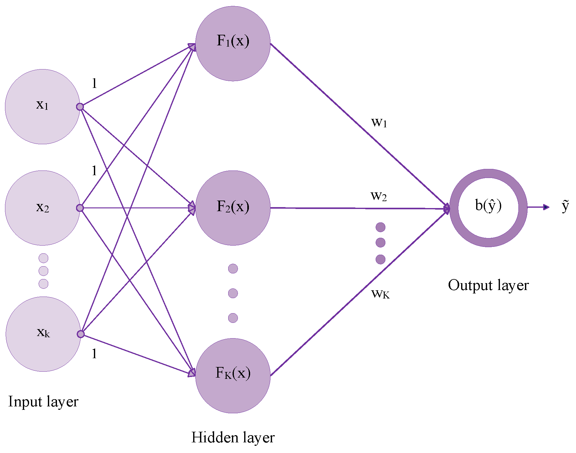
2. The FCI-WASD Classification Neural Network

In this section, we shall present the main components on which the structuring of the FCI-WASD is based. Specifically, we shall present the methods by which the neural network’s activations, hidden layer and optimal weights are determined. The FCI-WASD is a multi-input, 3-layer feed-forward neural network, whose final structure resembles that of Figure 1.

Inline with Figure 1, suppose that a classification dataset x comprises of k features, where $x_j\in {\mathbb{R}}^m,j=1,2,\dots ,k$ denotes the jth column of x. All feature columns are passed onto the hidden layer with a weight of 1. The neural network develops a hidden layer of $K\in \mathbb{N}$ neurons, where each neuron $i=1,2,\dots ,K$ represents the image of the input matrix $x=\left[\begin{array}{c}{x}_1,x_2,\dots ,x_k\end{array}\right]$ under the activation function $F_i$. Given a response column $y\in {\mathbb{R}}^m$ which acts as a benchmark, the weights direct determination (WDD) process, the defining feature of any WASD algorithm, assigns to each neuron i a corresponding weight $w_i$. The weighted combination of all K neurons produces a column vector $\widehat{y}\in \mathbb{N}$ which is then mapped to a binary vector $\tilde{y}$, the neural network’s final prediction. The conversion of $\widehat{y}$ to $\tilde{y}$ is done through an elementwise operator b:

$${\tilde{y}}_i=b_i\left(\widehat{y}\right)=\left\{\begin{array}{c}1,{\widehat{y}}_i\ge \tilde{t}\hfill \\ 0,{\widehat{y}}_i<\tilde{t}\hfill \end{array}\right.,i=1,2,\dots ,m$$

(1)

where, given a threshold $t\in [0,1]$, $\tilde{t}$ is defined as $\tilde{t}=min\widehat{y}+t(max\widehat{y}-min\widehat{y})$. Should the threshold t be picked close to 1, then only those entries of $\widehat{y}$ that are proportionally close to $max\widehat{y}$ are mapped to 1, with the opposite applying if we choose t to be on the lower end.

2.1. Fresnel Cosine Integral Activation Functions, Power Tables and the WDD Process

The WDD process, which is responsible for directly determining the optimal set of weights given a fixed number of neurons, opens the way for the simultaneous determination of the optimal overall structure, that is, the optimal number of neurons, whilst providing certainty that the obtained weights are indeed optimal. Thus, it successfully overcomes two of the key drawbacks of traditional BP methods, namely iterative as well as uncertain determination of the optimal weights and inability to obtain the optimal structure in a deterministic fashion [30,31].

With the determination of weights being safely handled, successfully encapturing the underlying relationship between an input matrix x and a target output y is now a question of developing a large enough structure that is coupled with appropriately chosen activation functions. When it comes to WASD neural networks, the choice of activation functions greatly impacts how the training process will unfold and, ultimately, how well the neural network will perform. Namely, being that $\widehat{y}$, prior to being converted to binary, is simply a weighted (linear) combination of K vectors where each vector is the image of the same input matrix x under an activation function $F_i$, there is a pressing need for those vectors to be linearly independent, else the neural network would not achieve much progress. As a result, in order to assert that the vectors comprising the weighted combination are linearly independent, it has been common practice to resort to power-based activation functions. For example, a number of polynomial activation functions, such as Euler, Bernoulli, Laguerre, Chebyshev, etc. were proposed in [31] whereas power-based activations such as the power, power sigmoid, power softplus, and power inverse exponential were proposed in [33].

When transitioning from single to multi-input WASD neural networks, the activation function $F_i$ corresponding to a given neuron no longer matches the initial function of choice raised to some power but is rather determined in a way that involves that function as a building block. In this paper, we shall investigate the implementation of the power Fresnel cosine integral as a sub-activation, that is to say, a building block for the neural network’s activation functions. The power Fresnel cosine integral is the Fresnel cosine integral, usually denoted by $C\left(x\right)$, raised to some power $n\in \mathbb{N}$:

$$C_n\left(x\right)={\left(C\left(x\right)\right)}^n={({\int }_0^{x}cos\left(\frac{\pi t^2}{2}\right)dt)}^n$$

(2)

Note that MATLAB’s Symbolic Math Toolbox has a built-in solution for calculating $C\left(x\right)$, namely, the fresnelc function. In Mathematica this is done through the FresnelC function and in Python this is implemented under scipy.special.fresnel, as part of the SciPy library. Raising the output of that function to some power is then straight-forward. As for the ability of the neural network to converge, one should take into cosnideration the following Definition 1, Theorem 1 and Proposition 1 from [31].

Definition 1.

Let $f(x_1,x_2,\dots ,x_k)$ be a function of k variables. The polynomials

$$B_{n_1{n}_2\cdots n_k}^f(x_1,x_2,\dots ,x_k)=\sum _{{\nu }_1=0}^{n_1}\cdots \sum _{{\nu }_k=0}^{n_k}f(\frac{{\nu }_1}{n_1},\cdots ,\frac{{\nu }_k}{n_k})\prod _{q=1}^k{C}_{n_q}^{{\nu }_q}{x}_q^{{\nu }_q}{(1-x_q)}^{n_q-{\nu }_q}$$

are called multivariate Bernstein polynomials of $f(x_1,x_2,\dots ,x_k)$, where $C_{n_q}^{{\nu }_q}$ denotes a binomial coefficient with $n_q=n_1,n_2,\dots ,n_k$ and ${\nu }_q=0,1,\dots ,n_q$.

Theorem 1.

Let $f(x_1,x_2,\dots ,x_k)$ be a continuous function defined over $V_k=\{(x_1,x_2,\dots ,x_k)\in {\mathbb{R}}^k|0\le x_q\le 1,q=1,2,\dots ,k\}$. Then the multivariate Bernstein polynomials $B_{n_1{n}_2\cdots n_k}^f(x_1,x_2,\dots ,x_k)$ converge uniformly to $f(x_1,x_2,\dots ,x_k)$ as $n_1,n_2,\dots ,n_k\to \infty$.

Proposition 1.

With a form of products of trigonometric power-based functions $C_n$ employed, we can construct a generalized trigonometric polynomial

$$F_i\left(x\right)=F_i(x_1,x_2,\dots ,x_k)=C_{n_{i1}}\left(x_1\right)C_{n_{i2}}\left(x_2\right)\cdots C_{n_{ik}}\left(x_k\right)=\prod _{j=1}^k{C}_{n_{ij}}\left(x_j\right),$$

for $i=1,2,\dots ,K$.

Proposition 1 lays the foundation for determining the activation function corresponding to the ith neuron. Thus, $F_i\left(x\right)$, or the image of the input matrix x under the ith activation, will comprise of the product of the images of the individual columns $x_j$ under Fresnel cosine integrals that are raised to integer powers $n_{ij}$, with $i=1,2,\dots ,K$ and $j=1,2,\dots ,k$. One now has to determine valid integers to be assigned to each $n_{ij}$ so that the neural network is able to function properly. In our experience, this assignment pattern has to be treated carefully as it can make or break a multi-input WASD neural network.

Suppose that we are dealing with a problem of k variables so that the input matrix x consists of k columns. In [31], it is suggested that the integers corresponding to the powers $n_{ij}$ should be drawn from a lexicographically ordered power table, that is, a predetermined $r\times k$ matrix $N_k$, with entries from $\mathbb{N}\cup \left\{0\right\}$, whose rows follow a certain ordering. To each neuron $i=1,2,\dots K$ will correspond a row in $N_k$ and to each variable $x_j,j=1,2,\dots ,k$, a column of powers in $N_k$. On that note, we shall write $n_{ij}=N_k(i,j)$. Notice that the number r of rows is usually greater than or equal to the final number of neurons K, as the former represents the initial target number of neurons that we wish for the neural network to accumulate and the latter corresponds to the optimal number of neurons to which the neural network settles by the end of the training process. This shall be further discussed in a later section. Finally, it should also be noted that the structuring of $N_k$ depends to some extent on the number of variables k, hence the subscript.

When it comes to single-input problems, constructing the table is straight-forward. Namely, $N_1$ is a $r\times 1$ vector with $N_1\left(i\right)=i-1,i=1,2,\dots ,r$. However, when it comes to problems of $k>1$ variables, an attempt to extend that simplistic pattern, say to $N(i,j)=i-1$ for all $j=1,2,\dots ,k$, would not do much for the network’s performance, as we can testify from experience. First things first, in accordance with the graded lexicographic ordering, as discussed in [31], a row $N_k^{\left(\beta \right)}=\left[\begin{array}{c}{n}_{\beta 1},n_{\beta 2},\dots ,n_{\beta k}\end{array}\right]$ of $N_k$ takes precedence over a different row $N_k^{\left(\alpha \right)}=\left[\begin{array}{c}{n}_{\alpha 1},n_{\alpha 2},\dots ,n_{\alpha k}\end{array}\right]$ if either of the following conditions is satisfied:

• C.I: ${\sum }_{j=1}^k{n}_{\alpha j}>{\sum }_{j=1}^k{n}_{\beta j}$;
• C.II: ${\sum }_{j=1}^k{n}_{\alpha j}={\sum }_{j=1}^k{n}_{\beta j}$ and the first nonzero entry of $N_k^{\left(\alpha \right)}-N_k^{\left(\beta \right)}$ is positive.

On determining the actual entries of $N_k$, ref. [31] provides a few samples for $N_k$ when $k\in \{1,2,3,4\}$. Due to the absence of further instructions, we have composed Algorithm 1, a heuristic algorithm, which aims at constructing $N_k$ for an arbitrary $k\in \mathbb{N}$. In terms of notation, we shall denote by $\sigma$ the sum of the elements of a row of $N_k$ and by $\Sigma$ an upper bound for $\sigma$. It is perhaps best that a few samples are given prior to the description of the algorithm thus, for the sake of illustration, let us set $\Sigma =2$. Then, the following are the first five power tables:

$$N_1=\left[\begin{array}{c}0\\ 1\\ 2\end{array}\right],N_2=\left[\begin{array}{cc}0& 0\\ 0& 1\\ 1& 0\\ 0& 2\\ 1& 1\\ 2& 0\end{array}\right],N_3=\left[\begin{array}{ccc}0& 0& 0\\ 0& 0& 1\\ 0& 1& 0\\ 1& 0& 0\\ 0& 0& 2\\ 0& 1& 1\\ 0& 2& 0\\ 1& 0& 1\\ 1& 1& 0\\ 2& 0& 0\end{array}\right],N_4=\left[\begin{array}{cccc}0& 0& 0& 0\\ 0& 0& 0& 1\\ 0& 0& 1& 0\\ 0& 1& 0& 0\\ 1& 0& 0& 0\\ 0& 0& 0& 2\\ 0& 0& 1& 1\\ 0& 0& 2& 0\\ 0& 1& 0& 1\\ 0& 1& 1& 0\\ 0& 2& 0& 0\\ 1& 0& 0& 1\\ 1& 0& 1& 0\\ 1& 1& 0& 0\\ 2& 0& 0& 0\end{array}\right],N_5=\left[\begin{array}{ccccc}0& 0& 0& 0& 0\\ 0& 0& 0& 0& 1\\ 0& 0& 0& 1& 0\\ 0& 0& 1& 0& 0\\ 0& 1& 0& 0& 0\\ 1& 0& 0& 0& 0\\ 0& 0& 0& 0& 2\\ 0& 0& 0& 1& 1\\ 0& 0& 0& 2& 0\\ 0& 0& 1& 0& 1\\ 0& 0& 1& 1& 0\\ 0& 0& 2& 0& 0\\ 0& 1& 0& 0& 1\\ 0& 1& 0& 1& 0\\ 0& 1& 1& 0& 0\\ 0& 2& 0& 0& 0\\ 1& 0& 0& 0& 1\\ 1& 0& 0& 1& 0\\ 1& 0& 1& 0& 0\\ 1& 1& 0& 0& 0\\ 2& 0& 0& 0& 0\end{array}\right].$$

Due to condition C.I of the graded lexicographic ordering rule, the rows of $N_k$ are sorted in ascending order according to the sum of their elements, that is, their $\sigma$. As a result, rows that share a common $\sigma$ are grouped together into $\sigma$-blocks, with the ordering within a given $\sigma$-block being defined by condition C.II. The heuristic element has to do with the contents of a given $\sigma$-block. Drawing from the samples in [31], which comprise of the previously given tables $N_1,N_2,N_3$ and $N_4$, it is perhaps not unreasonable to guess that a $\sigma$-block of $N_k$ will consist of all unique k-tuples, with entries from $\mathbb{N}\cup \left\{0\right\}$, whose elements sum to $\sigma$. On generating those tuples, we start from the k-tuple $\left[\begin{array}{c}\sigma ,0,\dots ,0\end{array}\right]$, which is an obvious candidate for any $\sigma$-block. Then we move to the vectors whose elements describe a unique integer partition for $\sigma$. For example, $\left[\begin{array}{c}3,0,\dots ,0\end{array}\right]$ is an obvious candidate for a block of $\sigma =3$ and $\left[\begin{array}{c}2,1,0,\dots ,0\end{array}\right]$, $\left[\begin{array}{c}1,1,1,0,\dots ,0\end{array}\right]$ are the two unique integer partitions of 3 in vector form. The block will then consist of all unique permutations of those three vectors. On a similar note, starting from an empty table $N_k$ and incrementing $\sigma$ from 0 to some upper bound $\Sigma$ whilst concatenating the resulting $\sigma$-blocks to the bottom of $N_k$, will yield as many rows of $N_k$ as we please so far as we choose $\Sigma$ to be large enough. Although that is the original idea, we may take it a step further so that we do not ever have to worry about choosing a valid $\Sigma$. Namely, we simply increment $\sigma$ whilst keeping track of the number of rows in $N_k$. We may stop as soon as the number r of rows in $N_k$ has surpassed a minimum threshold, $r_{min}$. The aforementioned process gives rise to Algorithm 1, which handles the task of the power table generation.

Algorithm 1 Creation of Power Tables
Require: minimum number of rows $r_{min}$, number of inputs k
1:	if $k==1$ then
2:	set $N_k={\left[\begin{array}{c}0,1,2,\dots ,r-1\end{array}\right]}^T$
3:	else
4:	initialize $N_k$ as an empty matrix and set $\sigma =-1$
5:	while number of rows in $N_k$ < $r_{min}$ do
6:	increment $\sigma$ by 1
7:	set $Ntemp$ to be an empty matrix
8:	compute the m unique integer partitions of $\sigma$ consisting of k integers $\ge 0$.
9:	for $i=1$ to m do
10:	compute, as rows, the unique permutations of each integer partition
11:	concatenate the resulting permutations to the bottom of $Ntemp$
12:	end for
13:	sort $Ntemp$ by C.II of the graded lexicographic order and concatenate it to the bottom of $N_k$
14:	end while
15:	end if
Ensure: $N_k$

The final crucial element which determines the success of the neural network is the WDD process, undoubtedly the single defining feature of WASD training algorithms. Letting $F=\left[\begin{array}{c}{F}_1\left(x\right),F_2\left(x\right),\dots ,F_K\left(x\right)\end{array}\right]$, where $F_i\left(x\right)$, $i=1,2,\dots ,K$, is the image of the input matrix x under the ith activation and also the ith column of the activation matrix F, determining the optimal weights $w_1,w_2,\dots ,w_K$ that connect the hidden to the output layer is equivalent to finding the optimal vector $w={\left[\begin{array}{c}{w}_1,w_2,\dots ,w_K\end{array}\right]}^T$ such that $w_1{F}_1\left(x\right)+w_2{F}_2\left(x\right)+\cdots +w_K{F}_K\left(x\right)=Fw=\widehat{y}$ is, in a least-squares sense, as close to the response column y as possible. By the WDD process [30], we have that:

$$w=F^{†}y,$$

(3)

where $F^{†}$ denotes the pseudo-inverse of F.

2.2. The WASD Training Algorithm of the FCI-WASD

WASD training algorithms aim at simultaneously handling both the determination of the optimal overall structure as well as the optimal set of weights corresponding to that structure. For any given size that we may consider for the hidden layer, the latter part of the problem is readily dealt with by use of the WDD process, as in Equation (3). Thus, all things considered, it is only necessary to formulate a strategy as to how the neural network will decide on an optimal number of hidden layer neurons.

It is worth noting that, contrary to weights determination, which is very specific, this part of the problem offers itself for improvisation and may be tackled through various approaches. Following are a few natural considerations which will directly influence the training path. Namely, one may ask:

• Which metric to use so as to keep track of training progress?
• How frequently will the training progress be monitored?
• What will the stopping criterion consist of?
• Will the network’s final structure retain all accumulated neurons?
• If not, then when and under which conditions should the neural network opt to discard neurons?

All things considered, making an educated decision is a process of trial and error which may depend on the type of the problem (be it regression or classification), on how much one wishes to prioritize performance over speed and vice versa, as well as on the dataset itself. Although it is hard to argue optimality in this context, we have settled on an approach which seems to favour classification performance. Namely, regarding question 1, the metric of choice is

$$\mathrm{MAE}=\frac{1}{m}\sum _{i=1}^m|{\tilde{y}}_i-y_i|,$$

(4)

where $\tilde{y}$ is the prediction of the neural network converted to binary, as in Equation (1). As far as considerations 2–4 are concerned, on incorporating the metric in the training process, a common approach is to iteratively increase the size of the hidden layer whilst updating the training metric. Then, newly added neurons are kept so far as they contribute to an increase in the neural network’s marginal performance. Finally, upon a predetermined number of iterations were no neurons were kept, the training process would come to an end. We have however abstained from such a practice as it not only adds a time toll due to $F^{†}$ being re-computed in each iteration but also because, in the context of $\mathrm{MAE}$, this approach leads to the neural network accumulating a disproportionately small number of neurons, thus hindering its generalization ability. Last but not least, regarding consideration 5, we instead opt to develop the hidden layer up to a predetermined number of neurons and only then trim non-necessary neurons. Therefore, evaluation of the network’s $\mathrm{MAE}$ will start taking place only on the latter half of the training process.

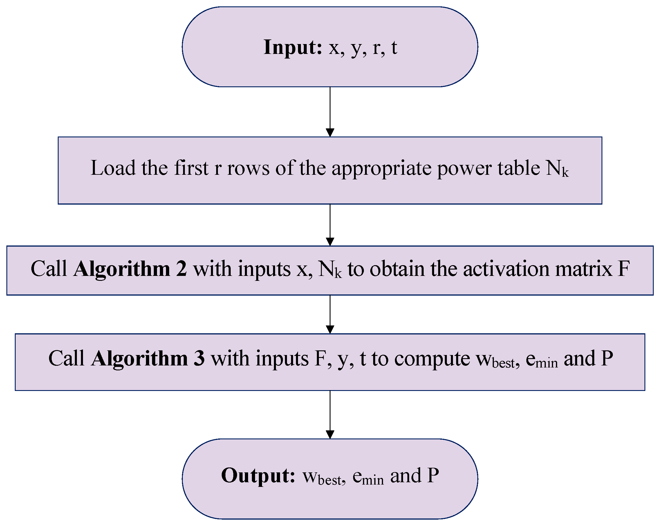
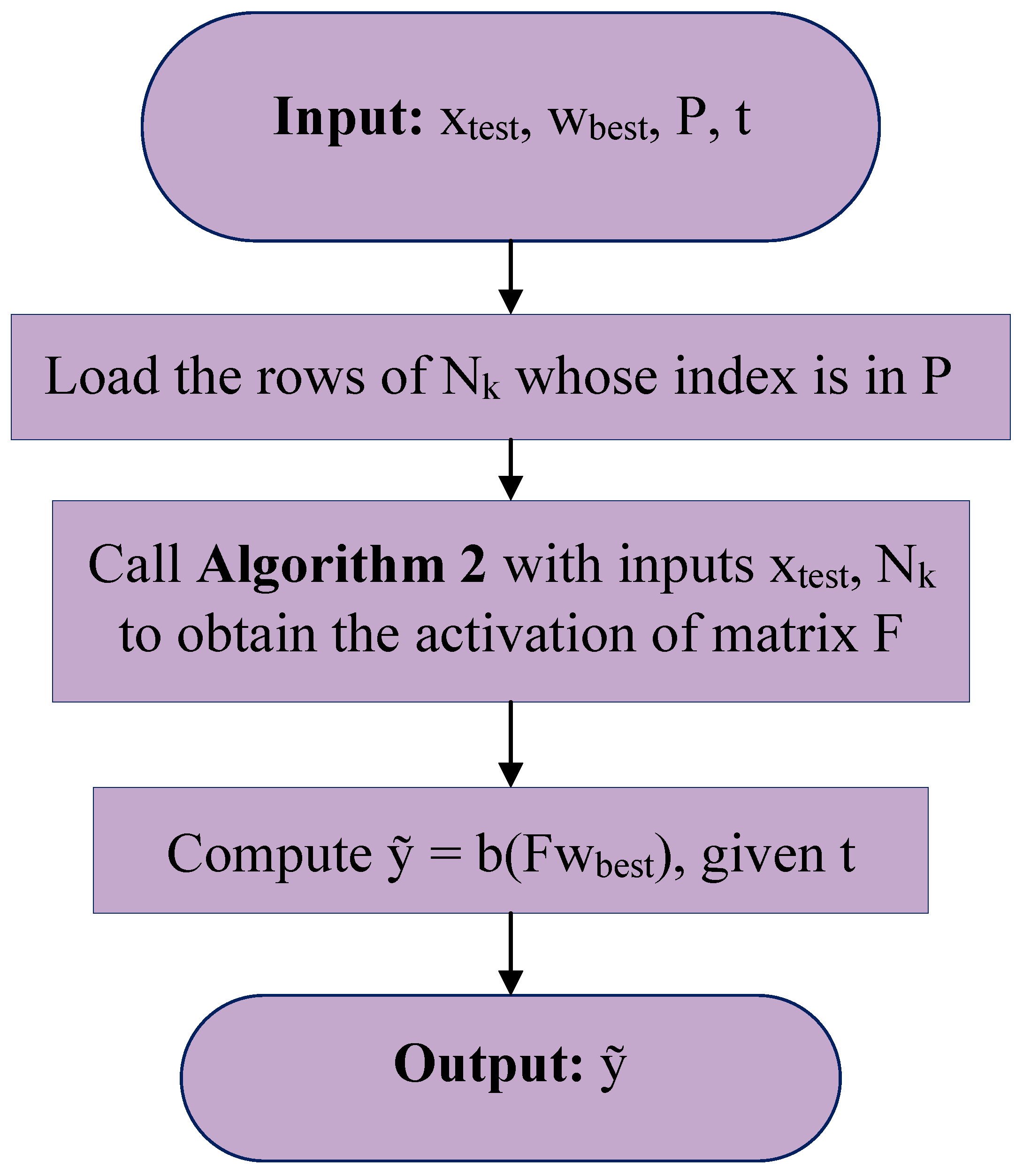
The Step by Step Process Cycle of Constructing and Employing the FCI-WASD

Step 1: The first step of the process, which consists of growing the hidden layer up to a given size, is handled by Algorithm 2. The algorithm inevitably includes substantial MATLAB functionality and notation [34]. It bears mentioning that, due to the nature of the power table $N_k$ where along any column $j=1,2,\dots ,k$ one stumbles upon many repetitions of a given power $n_{ij}$, computation of some $C_{n_{ij}}\left(x_j\right)$, as in Proposition 1, that has already been computed comes up very often. Thus, caching previously computed results, that is, employing memoization, will pay off handsomely in cutting down the total running time as most of the components of each $F_i\left(x\right)$ will be readily available and expensive computations will be kept to a minimum. This will also greatly offset the computational burden that the evaluation of Fresnel integrals entails, as opposed to the evaluation of a simpler function. We implement the memo as a 3D matrix. Namely, to each one of the k columns of x corresponds a $m\times (\Sigma +1)$ matrix whose rows match the number of samples in x. Being that $\Sigma$, as discussed previously, is an upper bound for the $\sigma$ and thus the power that may come up in a given power table $N_k$, we allocate $\Sigma +1$ columns to account for all those powers, including the power 0. Upon computation of some $C_{n_{ij}}\left(x_j\right)$, the resulting output will be stored in the $n_{ij}+1$ column of the jth matrix. Collectively, those matrices form a $m\times (\Sigma +1)\times k$ matrix, the memo. With the goal being to compute the activation matrix F that is associated with a target number of neurons, we do that column by column, as in Proposition 1, whilst utilizing the memo to accelerate the whole process. The full implementation is presented in Algorithm 2.

Algorithm 2 Constructing the activation matrix F
Require: The matrix of inputs x, the power table $N_k$
1:	procedure ACTIVATIONMATRIX($x,N_k$)
2:	set $m,k$ the number of rows and columns, respectively, in x
3:	set r the number of rows in $N_k$ and set $\Sigma$ = sum($N_k(r,:)$)
4:	initialize the memo M as an $m\times (\Sigma +1)\times k$ NaN array
5:	set F = zeros$(m,r)$
6:	for $i=1$ to r do
7:	set f = zeros$(m,k)$
8:	for $j=1$ to k do
9:	set n = $N_k(i,j)$
10:	if sum(isnan($M(:,k+1,j)$)) == m then
11:	set $M(:,k+1,j)$ = $C_n\left(x(:,j)\right)$, as in Equation (2)
12:	end if
13:	set $f(:,j)$ = $M(:,k+1,j)$
14:	end for
15:	set $F(:,i)$ = prod(f,2)
16:	end for
17:	end procedure
Ensure: The matrix F

Step 2: The second step of the network building process comprises of fine tuning the structure that has been obtained from the previous stage. Namely, following the successful computation of the activation matrix F, the hidden layer of the neural network has now acquired sufficient size. At this point, we go through a trimming process in order to locate and drop those neurons that are no longer essential to the network’s performance. Namely, the neurons comprising the hidden layer are taken out one by one and the neural network’s $\mathrm{MAE}$ is computed. If at a given iteration this has resulted in a lower overall $\mathrm{MAE}$, then the neuron in question is permanently removed from the hidden layer. In the end, we will have acquired the indices of only the bare essential neurons and thus, coupled with the optimal set of weights obtained from Equation (3), we will have settled on an optimal overall structure. The aforementioned process is handled by Algorithm 3, which again includes some MATLAB functionality [34].

This concludes the weights and structure determination for the FCI-WASD. At the end of the process we will have acquired an optimal set of weights $w_{best}$ and a K element vector P, $K\le r$, that contains the positions of the remaining neurons. The final training error $e_{min}$ is the $\mathrm{MAE}$ associated with the given input matrix x which, along with the response column y, has served in the training of the neural network. The flowchart in Figure 2 presents the WASD algorithm, which follows the procedures of steps 1 and 2 and is responsible for the whole training process of the FCI-WASD.

Algorithm 3 Hidden layer trimming process
Require: The activation matrix F, the response vector y and a threshold $t\in [0,1]$
1:	$w_{\mathrm{best}}=F^{†}y$
2:	$\tilde{y}=b\left(Fw\right)$ given t, as in Equation (1)
3:	$e_{\min }=\frac{1}{m}{\sum }_{j=1}^m|{\tilde{y}}_j-y_j|$
4:	set r the number of columns in F
5:	$P=\left[\begin{array}{c}1,2,\dots ,r\end{array}\right]$
6:	for $i=1$ to r do
7:	kept = $\left[\begin{array}{c}1,\dots ,i-1,i+1,\dots ,r\end{array}\right]$
8:	f = $F(:,$kept)
9:	$w=f^{†}y$
10:	$\tilde{y}=b\left(fw\right)$
11:	$e=\frac{1}{m}{\sum }_{j=1}^m|{\tilde{y}}_j-y_j|$
12:	if $e_{\min }>e$ then
13:	$e_{\min }=e$
14:	$w_{\mathrm{best}}=w$
15:	P = kept
16:	end if
17:	end for
Ensure: The optimal weights vector $w_{\mathrm{best}}$, the final training $\mathrm{MAE}$, $e_{min}$ and the vector P containing the indices/positions of the essential neurons.

Step 3: The third and last step of the overall process cycle consists of employing the FCI-WASD so as to acquire predictions. Given new unseen data $x_{test}$, recreation and application of the FCI-WASD requires only that we have saved the weights vector $w_{best}$ and the index vector P. The testing workflow is depicted in the flowchart of Figure 3 and comprises of loading the rows of the power table $N_k$ corresponding to the indices in P and calling Algorithm 2 to compute the activation matrix F. Obtaining the prediction of the neural network will then consist of computing $\widehat{y}=F{w}_{best}$ and subsequently converting the output to the binary vector $\tilde{y}$ through Equation (1).

3. Applications on Employee Attrition Classification

In this section, the FCI-WASD is tested on two publicly available employee attrition datasets, which we shall refer to as EA.I and EA.II, respectively, and its performance is compared to that of five other classifiers—a different WASD neural network employing Chebyshev polynomials as activations and four well established models coming from MATLAB’s classification learner app. Both WASD neural networks were trained up to 100 neurons and their input was standardized by a z-score transform to a mean of 0 and a standard deviation of 1. Furthermore, the threshold parameter t was set, in both datasets, to 0.5 for both models. As for the MATLAB classifiers, we went with the default settings that are associated with each model through the classification learner app.

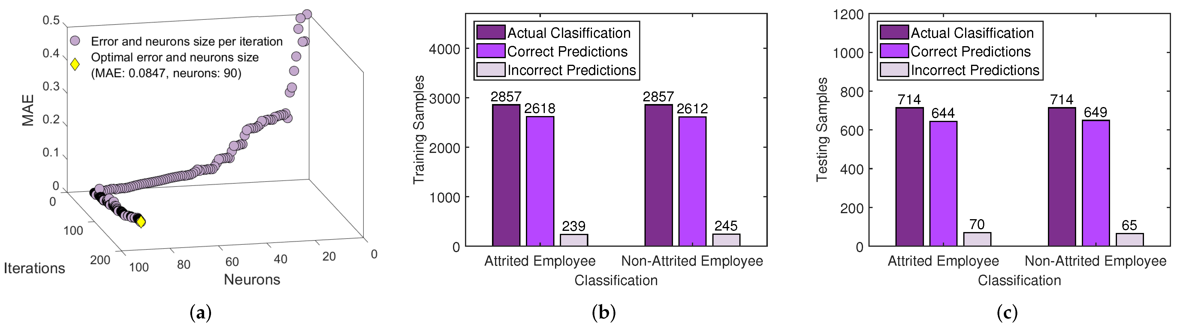
3.1. Employee Attrition Dataset I: Description and Preprocessing and Results of the FCI-WASD

The first dataset, available at [35], consists of 14,999 rows and 10 columns. It comes in near operational form as, except for the class imbalance in the response column, there are no missing values and most columns, except for columns 9 and 10 referring to the department and the salary status of each employee, are already numeric. In column 9 there are 10 unique departments listed like IT, accounting, HR, marketing, management, etc. On the other hand, column 10 lists 3 unique salary categories, namely high, medium and low. On converting all of these categories to meaningful numbers, we have resorted to the following approach for each of the two columns: For each category, we have counted the number of times that corresponding samples were mapped to employee attrition. We then normalized those counts to the interval $[-1,1]$, with categories showing higher counts being mapped closer to 1 and vice versa. Finally, those values were substituted back into the dataset. As was mentioned previously, the response column is imbalanced as it contains $76.19\%$ negative instances referring to non-attrited employees and only $23.81\%$ positive instances. On dealing with the class imbalance, we have employed a simple form of undersampling. We randomly sampled 7857 indices from 1 to 14,999 and dropped the corresponding rows. This resulted in a dataset with a 50-50 balance between attrited and non-attrited employees. Last but not least, the dataset was partitioned into a stratified 80–20% training and testing, respectively, split.

In Figure 4, the neural network’s training iterations Figure 4a, classification training Figure 4b and testing results Figure 4c are graphically presented. Given a target number of neurons (100), the first 100 iterations of Figure 4a correspond to the development of the activation matrix F, as in Algorithm 2, whereas the next 100 iterations refer to the hidden layer going through a trimming process, as in Algorithm 3. The training path taking a turn after the 100th iteration is a visual presentation of the neural network locating and dropping redundant neurons. Generally, the steepest the turn, the higher the number of neurons that are dropped during the trimming process whereas a down-sloping path connecting the starting and ending corners of the graph would imply that all accumulated neurons were kept. Last but not least, in terms of the training set, for attited and non-attrited employees alike, the FCI-WASD correctly classifies 2618 out of 2857 or $91.63\%$ of samples and 2612 out of 2857 or $91.42\%$ of samples, whereas in the testing set those percentages evaluate to 644 out of 714 or $90.19\%$ and 649 out of 714 or $90.89\%$ of samples, respectively. Thus, the FCI-WASD performs equally well as it correctly classifies the vast majority of instances of either category.

3.2. Employee Attrition Dataset II: Description, Preprocessing and Results of the FCI-WASD

The second dataset, available at [36], is significantly larger as it consists of 23,436 rows and 37 columns. However, 4 columns (columns 9, 10, 11, 23 and 28) with corresponding tags ‘EmployeeCount’, ‘EmployeeNumber’, ‘ApplicationID’, ‘Over18’, ’StandardHours’, were removed either because they displayed 0 variance (for example, ‘Over18’ was an array of straight 1s) or because they did not represent a valid predictor variable (for example, the ApplicationID column contains no useful information). Additionally, about 200 rows containing missing values were dropped along with 2 additional rows which contained an entry marked as ‘Test’. Other than that, the dataset requires some work to be brough into operational form. First things first, columns 2, 13 and 24 with tags ‘Attrition’ (the response column), ‘Gender’ and ‘OverTime’ were converted to binary, with 1s being assigned to resigned employees, to female employees (so as to account for the possibility of maternity leave) and to employees working overtime. Next, columns 3 (‘Business Travel’), 5 (‘Department’), 8 (‘EducationField’), 17 (‘JobRole’), 19 (‘MaritalStatus’) and 37 (‘EmployeeSource’) were converted to numeric in an identical manner to that described for columns 9 and 10 of the previous dataset. Finally, with only 3672 (or 15.83% of) samples corresponding to employees that resigned voluntarily, we randomly sampled and dropped enough indices so as to attain an even distribution between attrited and non-attrited employees. Again, for the purposes of training and testing, we resorted to a 80–20% stratified split.

In the same spirit with the previous example, Figure 5 contains a visual presentation of the neural network’s training iterations Figure 5a, as well as graphs of its performance in classifying employee attrition in the training Figure 5b and testing set Figure 5c, respectively. In this dataset the performance of the FCI-WASD is less satisfactory as the portion of misclassified samples has increased. Specifically, in the training set the neural network correctly classifies 2051 out of 2937, or $69.83\%$ of attrited employees and 2075 out of 2937, or $70.65\%$ of non-attrited employees. When it comes to the testing set, the respective percentages evaluate to 487 out of 734 and 555 out of 734, that is, $66.34\%$ and $75.61\%$, respectively. Nevertheless, all the other models show the same tendency when applied to EA.II, therefore it may be that the underlying reasons for this shortcoming are dataset specific rather than model specific.

3.3. Collective Results, Model Comparison and Statistical Tests

Following,

Table 1. Collective results of all models on the testing set of each dataset.

Model Dataset	FCI-WASD		Chebyshev WASD		Coarse Tree
	EA.I	EA.II	EA.I	EA.II	EA.I	EA.II
MAE	0.09453	0.29019	0.12255	0.33038	0.11415	0.34401
TP	0.90896	0.75613	0.94118	0.83515	0.94258	0.67302
FP	0.09103	0.24387	0.05882	0.16485	0.05742	0.32698
TN	0.90196	0.66349	0.81373	0.50409	0.82913	0.63896
FN	0.09803	0.33651	0.18627	0.49591	0.17087	0.36104
Precision	0.90896	0.75613	0.94118	0.83515	0.94258	0.67302
Recall	0.90264	0.69202	0.83478	0.62743	0.84654	0.65086
Accuracy	0.90546	0.70981	0.87745	0.66962	0.88585	0.65599
F-measure	0.90579	0.72266	0.88479	0.71654	0.89198	0.66175
Model Dataset	KNB		LR		Linear SVM
	EA.I	EA.II	EA.I	EA.II	EA.I	EA.II
MAE	0.14426	0.32629	0.23459	0.30245	0.21499	0.29837
TP	0.81373	0.55995	0.80392	0.68665	0.87395	0.68529
FP	0.18627	0.44005	0.19608	0.31335	0.12605	0.31471
TN	0.89776	0.78747	0.72689	0.70845	0.69608	0.71798
FN	0.10224	0.21253	0.27311	0.29155	0.30392	0.28202
Precision	0.81373	0.55995	0.80392	0.68665	0.87395	0.68529
Recall	0.88838	0.72487	0.74642	0.70195	0.74197	0.70845
Accuracy	0.85574	0.67371	0.76541	0.69755	0.78501	0.70163
F-measure	0.84942	0.63182	0.77411	0.69421	0.80257	0.69668

collectively depicts the individual performance of each model, as evaluated by means of nine metrics on the testing set of each of the two datasets. Four of those metrics, namely True Positive (TP), True Negative (TN), False Positive (FP) and False Negative (FN) serve as building blocks for determining the other five key metrics. On comparing the classifiers we shall only discuss their performance in terms of the latter. All things considered, the FCI-WASD has outperformed the other competing models as it scores the highest in 4 out of 5 and 3 out of 5 metrics in EA.I and EA.II, respectively. Namely, in EA.I it scores the lowest MAE ($9.45\%$) as well as the highest Recall ($90.26\%$), Accuracy ($90.54\%$) and F-measure ($90.57\%$). In terms of precision it scores $90.89\%$ and thus comes second after the Coarse Tree and the Chebyshev WASD which scored $94.25\%$ and $94.11\%$, respectively. As far as EA.II is concerned, all classifiers suffer a drop in performance but nevertheless the FCI-WASD again scores the lowest MAE ($29.01\%$), the highest Accuracy ($70.98\%$) and the highest F-measure ($72.26\%$). The Chebyshev WASD achieves the highest precision ($83.51\%$) over the FCI-WASD which scores $75.61\%$ and comes second on that metric. Last but not least, in the Recall department the KNB, Linear SVM and LR score the three highest scores which evaluate to $72.48\%$, $70.84\%$ and $70.19\%$, respectively.

In order to put these results into firmer ground, a statistical component, in the form of a mid p-value McNemar test [37], is added to the analysis. Namely, through a McNemar test one may be able to draw conclusions as to whether the predictive performances of two models, as measured by Accuracy, are different in a statistically significant manner. Thus, the null-hypothesis states that the accuracies of two classifiers are equal whereas the alternative hypothesis argues that this is not so. For each of the two datasets, the test shall be conducted by means of MATLAB’s testcholdout function which comes with the Statistics and Machine Learning Toolbox and we shall consider all possible pairs consisting of the FCI-WASD and one of the other classifiers. The collective outcomes of the McNemar tests are listed in

Table 2. McNemar test for the FCI-WASD.

FCI-WASD vs.	EA.I		EA.II
	Null Hypothesis	p-Value	Null Hypothesis	p-Value
Coarse Tree	Rejected	0.018056	Rejected	3.757 × 10${}^{-5}$
KNB	Rejected	1.7245 × 10${}^{-6}$	Rejected	0.010873
LR	Rejected	1.3126 × 10${}^{-29}$	Not rejected	0.29788
Linear SVM	Rejected	3.1406 × 10${}^{-25}$	Not rejected	0.49207
Chebyshev WASD	Rejected	0.00016552	Rejected	0.00055711

. As far as the first dataset is concerned, at the $5\%$ significance level the null hypothesis was rejected for all pairs, thus we may argue that the FCI-WASD has achieved superior accuracy on that dataset. When it comes to EA.II, the null hypothesis is rejected when comparing the accuracy of the FCI-WASD to that of the Coarse Tree, KNB and the Chebyshev WASD, however this is not the case for the LR and Linear SVM. Thus, on the second dataset, the FCI-WASD seems to have displayed equal accuracy, rather than superior, to that of the latter two models.

On the broader context where the rest of the metrics are taken into consideration, one may still argue that the FCI-WASD has performed better overall. Thus, given the need to test on a new stream of data coming from those sources, the results suggest that the FCI-WASD should be the first consideration out of the other five classifiers.

4. Conclusions

In view of employee attrition classification, this paper discusses the FCI-WASD, a classification neural network whose activation functions are formed through products of Fresnel cosine integrals, with each term in the product being raised to an integer power based of a lexicographically ordered power table. On comparing the neural network with other well established classifiers, we have considered two publicly available datasets and, following necessary preprocessing and class balancing steps, we have presented the collective results regarding the performance of the FCI-WASD versus that of five other classification models. The FCI-WASD achieves superior overall performance, that is, higher accuracy, MAE and F-measure scores than the rest of the models on both datasets, whereas the subsequent statistical analysis, in the form of a series of McNemar tests, argues that, in the vast majority of cases, those differences in accuracy are in fact statistically significant. Therefore, the FCI-WASD, as developed throughout the paper, is appropriate to take up the task of employee attrition classification.

The fact that only two datasets were considered is arguably a limitation in the study. Nevertheless, some areas of future research may be pointed out:

• Extension of the FCI-WASD to a multi-layer neural network could perhaps boost its performance and thus may be worth investigating.
• An ensemble classifier consisting of WASD models may also lead to a high performance model, therefore such a task may be worth considering.
• One could also investigate the comparison between WASD and radial basis function neural networks, or even experimenting with other transfer functions other than Fresnel cosine integrals, such as sigmoid, softplus, etc.
• Finally, to have the chance to test the FCI-WASD on an even larger, real world dataset, would be both a challenge as well as a tremendous opportunity that would help in asserting with confidence whether the model has stepped in the right direction as well as whether it is capable of bringing value to a company.

References

1. Alsheref, F.K.; Fattoh, I.E.; M Ead, W. Automated prediction of employee attrition using ensemble model based on machine learning algorithms. Comput. Intell. Neurosci. 2022, 2022, 7728668. [Google Scholar] [CrossRef]
2. Sexton, R.S.; McMurtrey, S.; Michalopoulos, J.O.; Smith, A.M. Employee turnover: A neural network solution. Comput. Oper. Res. 2005, 32, 2635–2651. [Google Scholar] [CrossRef]
3. Al-Darraji, S.; Honi, D.G.; Fallucchi, F.; Abdulsada, A.I.; Giuliano, R.; Abdulmalik, H.A. Employee attrition prediction using deep neural networks. Computers 2021, 10, 141. [Google Scholar] [CrossRef]
4. Hom, P.W.; Lee, T.W.; Shaw, J.D.; Hausknecht, J.P. One hundred years of employee turnover theory and research. J. Appl. Psychol. 2017, 102, 530–545. [Google Scholar] [CrossRef] [PubMed]
5. Zhao, Y.; Hryniewicki, M.K.; Cheng, F.; Fu, B.; Zhu, X. Employee turnover prediction with machine learning: A reliable approach. In Proceedings of the SAI Intelligent Systems Conference, London, UK, 6–7 September 2018; pp. 737–758. [Google Scholar] [CrossRef]
6. Mansor, N.; Sani, N.S.; Aliff, M. Machine learning for predicting employee attrition. Int. J. Adv. Comput. Sci. Appl. 2021, 12, 435–445. [Google Scholar] [CrossRef]
7. Simos, T.E.; Mourtas, S.D.; Katsikis, V.N. Time-varying Black-Litterman portfolio optimization using a bio-inspired approach and neuronets. Appl. Soft Comput. 2021, 112, 107767. [Google Scholar] [CrossRef]
8. Leung, M.F.; Wang, J. Cardinality-constrained portfolio selection based on collaborative neurodynamic optimization. Neural Netw. 2022, 145, 68–79. [Google Scholar] [CrossRef]
9. Leung, M.F.; Wang, J. Minimax and biobjective portfolio selection based on collaborative neurodynamic optimization. IEEE Trans. Neural Netw. Learn. Syst. 2021, 32, 2825–2836. [Google Scholar] [CrossRef]
10. Bai, L.; Zheng, K.; Wang, Z.; Liu, J. Service provider portfolio selection for project management using a BP neural network. Ann. Oper. Res. 2022, 308, 41–62. [Google Scholar] [CrossRef]
11. Yaman, I.; Dalkılıç, T.E. A hybrid approach to cardinality constraint portfolio selection problem based on nonlinear neural network and genetic algorithm. Expert Syst. Appl. 2021, 169, 114517. [Google Scholar] [CrossRef]
12. Mourtas, S.D.; Katsikis, V.N. Exploiting the Black-Litterman framework through error-correction neural networks. Neurocomputing 2022, 498, 43–58. [Google Scholar] [CrossRef]
13. Katsikis, V.N.; Mourtas, S.D. Diversification of time-varying tangency portfolio under nonlinear constraints through semi-integer beetle antennae search algorithm. AppliedMath 2021, 1, 63–73. [Google Scholar] [CrossRef]
14. Katsikis, V.N.; Mourtas, S.D. Computational Management. In Modeling and Optimization in Science and Technologies; Chapter Portfolio Insurance and Intelligent Algorithms; Springer: Cham, Switzerland, 2021; Volume 18, pp. 305–323. [Google Scholar] [CrossRef]
15. Mourtas, S.D.; Katsikis, V.N.; Drakonakis, E.; Kotsios, S. Stabilization of stochastic exchange rate dynamics under central bank intervention using neuronets. Int. J. Inf. Technol. Decis. 2023, 22, 855–883. [Google Scholar] [CrossRef]
16. Simos, T.E.; Katsikis, V.N.; Mourtas, S.D. Multi-input bio-inspired weights and structure determination neuronet with applications in European Central Bank publications. Math. Comput. Simul. 2022, 193, 451–465. [Google Scholar] [CrossRef]
17. Guo, D.; Nie, Z.; Yan, L. Novel discrete-time Zhang neural network for time-varying matrix inversion. IEEE Trans. Syst. Man Cybern. Syst. 2017, 47, 2301–2310. [Google Scholar] [CrossRef]
18. Jin, L.; Zhang, Y.; Li, S. Integration-enhanced Zhang neural network for real-time-varying matrix inversion in the presence of various kinds of noises. IEEE Trans. Neural Netw. Learn. Syst. 2016, 27, 2615–2627. [Google Scholar] [CrossRef]
19. Mao, M.; Li, J.; Jin, L.; Li, S.; Zhang, Y. Enhanced discrete-time Zhang neural network for time-variant matrix inversion in the presence of bias noises. Neurocomputing 2016, 207, 220–230. [Google Scholar] [CrossRef]
20. Liao, B.; Xiao, L.; Jin, J.; Ding, L.; Liu, M. Novel complex-valued neural network for dynamic complex-valued matrix inversion. J. Adv. Comput. Intell. Intell. Inform. 2016, 20, 132–138. [Google Scholar] [CrossRef]
21. Chen, K.; Yi, C. Robustness analysis of a hybrid of recursive neural dynamics for online matrix inversion. Appl. Math. Comput. 2016, 273, 969–975. [Google Scholar] [CrossRef]
22. Zhang, Y.; Jin, L.; Guo, D.; Fu, S.; Xiao, L. Three nonlinearly-activated discrete-time ZNN models for time-varying matrix inversion. In Proceedings of the 8th International Conference on Natural Computation, Chongqing, China, 29–31 May 2012; pp. 163–167. [Google Scholar] [CrossRef]
23. Jia, L.; Xiao, L.; Dai, J.; Cao, Y. A novel fuzzy-power zeroing neural network model for time-variant matrix Moore-Penrose inversion with guaranteed performance. IEEE Trans. Fuzzy Syst. 2021, 29, 2603–2611. [Google Scholar] [CrossRef]
24. Precup, R.E.; Tomescu, M.L.; Preitl, S.; Petriu, E.M. Fuzzy logic-based stabilization of nonlinear time-varying systems. Int. J. Artif. Intell. 2009, 3, 24–36. [Google Scholar]
25. Precup, R.E.; Tomescu, M.L.; Dragos, C.A. Stabilization of Rössler chaotic dynamical system using fuzzy logic control algorithm. Int. J. Gen. Syst. 2014, 43, 413–433. [Google Scholar] [CrossRef]
26. Huang, C.; Jia, X.; Zhang, Z. A modified back propagation artificial neural network model based on genetic algorithm to predict the flow behavior of 5754 aluminum alloy. Materials 2018, 11, 855. [Google Scholar] [CrossRef] [PubMed] [Green Version]
27. Wang, H.; Liu, P.X.; Liu, S. Adaptive neural synchronization control for bilateral teleoperation systems with time delay and backlash-like hysteresis. IEEE Trans. Cybern. 2017, 47, 3018–3026. [Google Scholar] [CrossRef] [PubMed]
28. Zhang, Y.; Wang, J. Obstacle avoidance of redundant manipulators using a dual neural network. In Proceedings of the IEEE International Conference on Robotics and Automation (Cat. No.03CH37422), Taipei, Taiwan, 14–19 September 2003; Volume 2, pp. 2747–2752. [Google Scholar] [CrossRef]
29. Zhang, Y.; Wu, H.; Zhang, Z.; Xiao, L.; Guo, D. Acceleration-level repetitive motion planning of redundant planar robots solved by a simplified LVI-based primal-dual neural network. Robot. Comput.-Integr. Manuf. 2013, 29, 328–343. [Google Scholar] [CrossRef]
30. Zhang, Y.; Yu, X.; Xiao, L.; Li, W.; Fan, Z.; Zhang, W. Weights and structure determination of articial neuronets. In Self-Organization: Theories and Methods; Nova Science: New York, NY, USA, 2013. [Google Scholar]
31. Zhang, Y.; Chen, D.; Ye, C. Deep Neural Networks: WASD Neuronet Models, Algorithms, and Applications; CRC Press: Boca Raton, FL, USA, 2019. [Google Scholar]
32. Simos, T.E.; Katsikis, V.N.; Mourtas, S.D. A fuzzy WASD neuronet with application in breast cancer prediction. Neural Comput. Appl. 2021, 34, 3019–3031. [Google Scholar] [CrossRef]
33. Simos, T.E.; Katsikis, V.N.; Mourtas, S.D. A multi-input with multi-function activated weights and structure determination neuronet for classification problems and applications in firm fraud and loan approval. Appl. Soft Comput. 2022, 127, 109351. [Google Scholar] [CrossRef]
34. Gupta, A.K. Numerical Methods Using MATLAB; MATLAB Solutions Series, Berkley; Springer Press: New York, NY, USA, 2014. [Google Scholar]
35. HR Dataset. Available online: https://www.kaggle.com/datasets/kadirduran/hr-dataset?resource=download. (accessed on 2 February 2023).
36. Capstone Project-IBM Employee Attrition Prediction. Available online: https://www.kaggle.com/datasets/rushikeshghate/capstone-projectibm-employee-attrition-prediction?resource=download. (accessed on 2 February 2023).
37. Fagerland, M.W.; Lydersen, S.; Laake, P. The McNemar test for binary matched-pairs data: Mid-p and asymptotic are better than exact conditional. BMC Med. Res. Methodol. 2013, 13, 91. [Google Scholar] [CrossRef] [PubMed] [Green Version]
Figure 1. Overview of the final structure of the FCI-WASD.
Mathematics 11 01506 g001
Figure 2. Flowchart for the training process of the FCI-WASD: The WASD algorithm.
Mathematics 11 01506 g002
Figure 3. Flowchart for the testing process of the FCI-WASD.
Mathematics 11 01506 g003
Figure 4. Training iterations and classification results of the FCI-WASD on EA.I. (a) EA.I: Training iterations; (b) EA.I: Training results; (c) EA.I: Testing results.
Mathematics 11 01506 g004
Figure 5. Training iterations and classification results of the FCI-WASD on EA.II. (a) EA.II: Training iterations; (b) EA.II: Training results; (c) EA.II: Testing results.
Mathematics 11 01506 g005