Refined Green–Lindsay Model for the Response of Skin Tissue under a Ramp-Type Heating

Abstract

Based on Green–Lindsay generalized thermoelasticity theory, this paper presents a new refined higher-order time-derivative thermoelasticity model. Thinner one-dimensional skin tissue is considered when its inner surface is free of traction and does not show any temperature increase. The skin tissue’s bounding surface has been heated by ramp-type heating. The classical thermoelastic theories are obtained from the present general formula. The governing equations of the present model are obtained. To move the system into a space state, the Laplace transform is used. The inverse of the Laplace transform is also used with Tzuo’s method to solve the problem. As a result, the field quantities are obtained numerically, and the results of the current model are graphically represented with a comparison to two different theories of thermoelasticity. The effects of various parameters on thermomechanical waves through the skin tissue are analyzed. The theory notes a vibrational behavior in heat transfer and a different effect on the parameters discussed in this article.

1. Introduction

Many medical treatments depend on the biothermal response to transfer heat through thermoelastic skin tissues, so understanding heat transfer is essential for both theoretical and practical applications. One of the most important aims of studying skin bio-thermoelasticity is to investigate the therapeutic effect of applying heat to the skin’s surface to treat the target tissues without affecting the surrounding tissues. The investigation of the bio-thermoelastic response of living tissue utilizes a new and efficient generalized thermoelasticity model based on the Green–Lindsay (G–L) theory. The model presented here will allow predictions of bio-thermoelastic tissue which is an important effect. Most bio-heat transfer theories are created according to the classical Fourier’s law, which describes extremely fast thermal signal propagation. In recent literature, a variety of bio-heat transfer theories have been developed for skin tissue, including Pennes’s theory [1], thermal wave (TW) theory, and dual-phase-lag (DPL) theory [2]. The linear theory of coupled thermoelasticity (CTE) was satisfactorily derived by Biot [3], who also proposed a theory of irreversible thermodynamics. Lord and Shulman (L–S) [4], Green and Lindsay [5], and others attempted to alter the CTE theory on various grounds to produce a wave-type heat conduction equation to deal with this contradiction. Through an experiment, Mitra et al. [6] investigated the wave-like response of heat transfer in biological tissues.

Different investigators have demonstrated that each of the DPL and TW theories can stimulate other non-physical properties. Antaki [7] used the DPL theory to explain the heat conduction in dealing with meat which was explained with the TW theory. Liu and Lin [8] presented an inverse analysis of bi-layer spherical tissue. Xu et al. [9,10,11] discussed the application of bio-heat transfer models in the bio-thermomechanical effect of skin tissue. Ng et al. [12] developed the boundary element method for the bio-heat transfer problems within heated human skin. Kundu and Dewanjee [13] examined the non-Fourier and Fourier thermal behaviors in single-layer, one-dimensional skin tissue. Shih et al. [14] discussed the parabolic Pennes’ bioheat formula under oscillatory heat flux at the skin tissue. Ghazizadeh et al. [15] used the fractional thermal wave (FTW) bio-heat transfer formula to develop the non-Fourier behavior. In Ezzat and El-Karamany [16], two general models of fractional heat conduction for non-homogeneous anisotropic elastic solids were discussed. Jiang and Qi [17] discussed heat transfer in biological tissue utilizing the FTW bio-heat transfer equation. Ezzat et al. [18] discussed the tissue behavior on the skin surface utilized in the FTW bio-heat transfer equation. For a perfect conducting solid with a time-fractional derivative in one dimension, Ezzat et al. [19] develop a mathematical model of the equations of the two-temperature magneto-thermoelasticity theory. Utilizing the fractional DPL theory, Kumar and Rai [20] explored the thermal response in living biological tissues. In a medium containing a spherical cavity under two phases of G–L theory, Kumar et al. [21] analyzed the impact of temperature-dependent thermal conductivity on thermoelastic interactions. Chyr and Shynkarenko [22] formulated the corresponding variational problem based on the G–L initial-boundary-value problem of thermoelasticity, sufficient conditions for initial data regularity, and proved the uniqueness of its solution and the existence of the generalized solution. Quintanilla [23] showed a modification of the G–L theory and discussed some qualitative results of it.

A single-layer skin tissue exposed unexpectedly to heat source issues as well as three-layer skin tissue has been discussed by Goudarzi and Azimi [24] in connection with a hot water source. A triple-phase-lag (TPL) model was proposed by Kumar et al. [25] to explain heat transfer in skin tissue with a finite domain with temperature-dependent metabolic heat generation. To examine the bio-thermo-mechanics behavior in living tissue and apply the model to a problem of a cancerous layer, Ezzat [26] used the fractional model of the thermo-viscoelasticity theory. The FTW of the bio-heat transfer equation is also utilized by Du et al. [27] to discuss the temperature and heat transfer mechanism of living biological tissues with fixed thickness subjected to a short-pulse laser. Youssef and Alghamdi [28] introduced a mathematical model of thermoelastic skin tissue utilizing the DPL heat conduction law. Using the refined L–S heat conduction equation, Sobhy and Zenkour [29] presented a mathematical model of thermoelastic on one-layer skin tissue. The thermal reaction and response of skin tissue exposed to a steady heat flux as a consequence of thermo-electrical shock on the bounding plane were studied by Youssef and Salem [30]. Ezzat and Alabdulhadi [31] presented a mathematical model of generalized thermo-viscoelasticity theory based on Pennes’ bioheat transfer equation with DPL to treat skin tumors by local hyperthermia. Based on a TPL model, Zhang et al. [32,33] examined the thermal response of skin tissue and the thermoelastic behaviors of biological tissue under thermal shock. Bioheat transmission and heat caused by a mechanical response in bi-layered human skin were investigated by Li et al. [34] using the Green–Naghdi model II (G–N model II) of thermoelasticity. To give a quantitative and systematic analysis to solve the nonlinear thermoelastic equation, Shakeriaski et al. [35] introduced the stress rate and temperature rate to the G–L model’s governing equations. In the context of the refined G–L theory of generalized thermoelasticity with strain rate, Sarkar et al. [36] published a study on the reflection and spread of harmonic plane waves. Filopoulos et al. [37] derived thermoelastic models for materials and provided a model to generalize G–L theory for linear elastic materials with microstructure.

Due to the development and modifications in the theories of thermodynamics and their uses in bio-mathematics, we developed a new modified model of the G–L theory of thermoelasticity [29,38,39,40]. The coupled thermoelastic system equations of differential equations are obtained. The distributions of field quantities, such as temperature, stress, displacement, and dilatation, are investigated by using the refined G–L bio-heat transfer model. The effects due to the G–L relaxation times and other parameters on thermoelastic behaviors are discussed. This study aims to present an improved model of the G–L thermoelasticity theory, which is characterized by giving finite speeds of heat transfer and applying it to biological tissues and knowing how applied convection affects tissues.

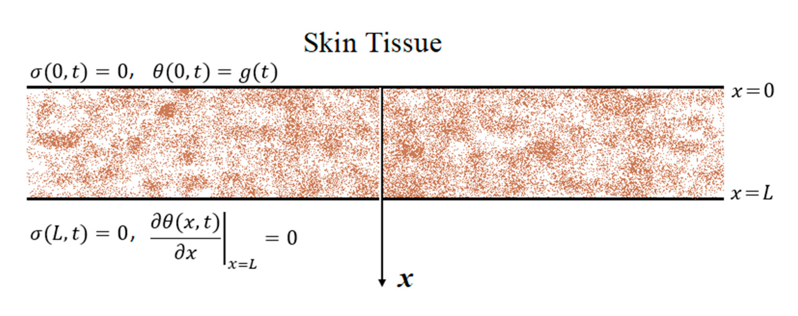
2. Governing Equations

The classical Fourier’s law [29,30,37] states connecting between heat flux vector $q_i$ and temperature gradient ${\theta }_{,i}$ by the equation

$$q_i=-k_t{\theta }_{,i},·····i=1,2,3.$$

(1)

Based on the coupling of the strain and temperature fields, the principle of local energy balance [32] gives

$$-q_{i,i}+Q={\rho }_t{c}_t\frac{\partial \theta }{\partial t}+{\gamma }_t{T}_b\frac{\partial e}{\partial t},$$

(2)

where $Q$ is the heat source.

The CTE theory [3] is one of the fundamental theories that studies coupled thermoelasticity in which we obtain the heat conduction equation by elimination of $q_i$ using Fourier’s law as

$$k_t{\nabla }^2\theta ={\rho }_t{c}_t\frac{\partial \theta }{\partial t}+{\gamma }_t{T}_b\frac{\partial e}{\partial t}-Q,$$

(3)

with equations of motion

$${{\mu }_{t}u}_{i,jj}+\left({\lambda }_t+{\mu }_t\right)u_{j,ji}-{\gamma }_t{\theta }_{,i}+{\rho }_t{f}_i={\rho }_t{\ddot{u}}_i.$$

(4)

Green and Lindsay [5] developed the energy equation and the equations of motion to avoid the contradiction of infinite speeds found in the CTE theory by adding two relaxation times for heat discouragement. The simple case of the G–L model is given by

$$k_t{\nabla }^2\theta ={\rho }_t{c}_t\left(1+{\tau }_1\frac{\partial }{\partial t}\right)\frac{\partial \theta }{\partial t}+{\gamma }_t{T}_{\mathrm{b}}\frac{\partial e}{\partial t}-Q,$$

(5)

with equations of motion

$${{\mu }_{t}u}_{i,jj}+\left({\lambda }_t+{\mu }_t\right)u_{j,ji}-{\gamma }_t\left(1+{\tau }_2\frac{\partial }{\partial t}\right){\theta }_{,i}+{\rho }_t{f}_i={\rho }_t{\ddot{u}}_i,$$

(6)

where ${\tau }_1$ is the first relaxation time, and ${\tau }_2$ is the second relaxation time that satisfies the inequalities ${\tau }_2\ge {\tau }_1\ge 0$. The refined form of the heat conduction equation for the G–L model is given by [41,42,43,44]

$$k_t{\nabla }^2\theta ={\rho }_t{c}_t\left(1+{\sum }_{n=1}^N\frac{{\tau }_1^n}{n!}\frac{{\partial }^n}{\partial t^n}\right)\frac{\partial \theta }{\partial t}+{\gamma }_t{T}_b\frac{\partial e}{\partial t}-Q,$$

(7)

with equations of motion in general form

$${{\mu }_{t}u}_{i,jj}+\left({\lambda }_t+{\mu }_t\right)u_{j,ji}-{\gamma }_t\left(1+{\sum }_{n=1}^N\frac{{\tau }_2^n}{n!}\frac{{\partial }^n}{{\partial t}^n}\right){\theta }_{,i}+{\rho }_t{f}_i={\rho }_t{\ddot{u}}_i.$$

(8)

From this model, the CTE theory can be obtained by replacing the relaxation times with zero in Equations (7) and (8). The simple case of G–L theory can also be obtained by substituting $N=1$ in the refined model.

To investigate the bio-thermoelasticity response of biological tissue, consider a one-dimensional (1D) skin tissue layer in which the outer surface is subjected to thermal loading of ramp-type heating and is traction free, while the inner surface is traction free and has no temperature change. As a result [28,29,30,31,32,33,34], the external heat source can be written as

$$Q=w_b{\rho }_b{c}_b\left(T_b-T\right)+Q_m+Q_L,$$

(9)

and the heat conduction equation becomes

$$k_t{\nabla }^2\theta ={\rho }_t{c}_t\left(1+{\sum }_{n=1}^N\frac{{\tau }_1^n}{n!}\frac{{\partial }^n}{{\partial t}^n}\right)\frac{\partial \theta }{\partial t}+{\gamma }_t{T}_b\frac{\partial e}{\partial t}+w_b{\rho }_b{c}_b\theta -Q_m-Q_L,\hspace{1em}N\ge 1,$$

(10)

with a 1D equation of motion and no external influences

$$\left({\lambda }_t+2{\mu }_t\right)\frac{{\partial }^{2}u}{{\partial x}^2}-{\gamma }_t\left(1+{\sum }_{n=1}^N\frac{{\tau }_2^n}{n!}\frac{{\partial }^n}{{\partial t}^n}\right)\frac{\partial \theta }{\partial x}={\rho }_t\frac{{\partial }^{2}u}{{\partial t}^2}.$$

(11)

For the present 1D case, the stress–strain and temperature relation will be reduced to

$$\sigma =\left({\lambda }_t+2{\mu }_t\right)e-{\gamma }_t\left(1+{\sum }_{n=1}^N\frac{{\tau }_2^n}{n!}\frac{{\partial }^n}{{\partial t}^n}\right)\theta ,$$

(12)

where

$$e=\frac{\partial u}{\partial x}.$$

(13)

3. Mathematical Solution to the Problem

Considering the refined G–L model, Equations (10)–(12) may be expressed as

$$\frac{{\partial }^{2}u}{\partial x^2}-c_1\left(1+{\sum }_{n=1}^N\frac{{\tau }_2^n}{n!}\frac{{\partial }^n}{\partial t^n}\right)\frac{\partial \theta }{\partial x}=\frac{1}{C_P^2}\frac{{\partial }^{2}u}{\partial t^2},$$

(14)

$$C_T^2\frac{{\partial }^2\theta }{\partial x^2}=\left(1+{\sum }_{n=1}^N\frac{{\tau }_1^n}{n!}\frac{{\partial }^n}{\partial t^n}\right)\frac{\partial \theta }{\partial t}+w_b{\rho }_c\theta +\eta \frac{{\partial }^{2}u}{\partial t\partial x}-Q_0,$$

(15)

$$\frac{\sigma }{{\lambda }_t+2{\mu }_t}=\frac{\partial u}{\partial x}-c_1\left(1+{\sum }_{n=1}^N\frac{{\tau }_2^n}{n!}\frac{{\partial }^n}{{\partial t}^n}\right)\theta ,$$

(16)

where

$$\begin{gathered} c_1=\frac{{\gamma }_t}{{\lambda }_t+2{\mu }_t},\cdots C_P^2=\frac{{\lambda }_t+2{\mu }_t}{{\rho }_t},\cdots C_T^2=\frac{k_t}{{\rho }_t{c}_t},\cdots {\rho }_c=\frac{{\rho }_b{c}_b}{{\rho }_t{c}_t}, \\ \eta =\frac{{\gamma }_t{T}_b}{{\rho }_t{c}_t},\cdots Q_0=\frac{Q_m}{{\rho }_t{c}_t},\cdots Q_L=0. \end{gathered}$$

(17)

The initial and boundary conditions for the problem will now be discussed. The initial conditions of the problem under consideration are assumed to be homogeneous as

$${\left.u(x,t)\right|}_{t=0}={\left.\frac{{\partial }^{n}u(x,t)}{\partial t^n}\right|}_{t=0}=0, {\left.\theta (x,t)\right|}_{t=0}={\left.\frac{{\partial }^n\theta (x,t)}{\partial t^n}\right|}_{t=0}=0,\hspace{1em}n\ge 1.$$

(18)

On both internal and external surfaces, the biological tissue is traction free. Thermal loading is applied to the skin tissue’s external surface, while the inner surface remains insulated without any heat transfer between the target biological tissue and the surrounding tissue. Hence, the boundary conditions are expressed as

$$\theta \left(0,t\right)=g\left(t\right),\hspace{1em}{\left.\frac{\partial \theta \left(x,t\right)}{\partial x}\right|}_{x=L}=0,\hspace{1em}\sigma \left(0,t\right)=0,\hspace{1em}\sigma \left(L,t\right)=0,$$

(19)

in which $g\left(t\right)$ is the function of thermal loading applied to the skin tissue’s outer surface $x=0$ as shown in Figure 1. Second, we suppose that ramp-type heating is utilized to the tissue’s plane $x=0$ as

$$g\left(t\right)={\theta }_0\left\{\begin{array}{ccc}\frac{t}{t_0}& \mathrm{i}\mathrm{f}& 0<t<t_0\\ 1& \mathrm{i}\mathrm{f}& t\ge t_0\end{array}\right.,$$

(20)

where $t_0>0$ is the parameter of ramp-type heating, and ${\theta }_0>0$ is a constant that denotes the thermal loading.

4. Laplace Transform Domain and Its Inversion

The Laplace transform is given by

$$\stackrel{-}{f}\left(x,s\right)={\int }_0^{\mathrm{\infty }}{\mathrm{e}}^{-st}f\left(x,t\right)\mathrm{d}t.$$

(21)

We constructed field equations in Laplace change space by applying the Laplace transform on both sides of Equations (14)–(16) and using homogeneous initial conditions (18)

$$\left(\frac{{\mathrm{d}}^2}{\mathrm{d}{x}^2}-2c_2\right)\stackrel{-}{u}=c_3\frac{\mathrm{d}\stackrel{-}{\theta }}{\mathrm{d}x},$$

(22)

$$\left(\frac{{\mathrm{d}}^2}{\mathrm{d}{x}^2}-2c_4\right)\stackrel{-}{\theta }=2c_5\frac{\mathrm{d}\stackrel{-}{u}}{\mathrm{d}x}-{\stackrel{-}{Q}}_1,$$

(23)

$$\frac{\stackrel{-}{\sigma }}{{\lambda }_t+2{\mu }_t}=\frac{\mathrm{d}\stackrel{-}{u}}{\mathrm{d}x}-c_3\stackrel{-}{\theta },$$

(24)

where

$$\begin{gathered} {\stackrel{-}{Q}}_1=\frac{{\stackrel{-}{Q}}_0}{s{C}_T^2},\cdots c_2=\frac{s^2}{2C_P^2},\cdots c_3=c_1\left(1+{\sum }_{n=1}^N\frac{{\tau }_2^n}{n!}{s}^n\right), \\ {c}_4=\frac{1}{{2C}_T^2}\left[w_b{\rho }_c+s\left(1+{\sum }_{n=1}^N\frac{{\tau }_1^n}{n!}{s}^n\right)\right],\cdots c_5=\frac{\eta s}{{2C}_T^2}. \end{gathered}$$

(25)

It should be noted that the over bar image denotes the Laplace transform, and the Laplace parameter is indicated by the small letter $s$.

Solving the system of equations that appeared in Equations (22) and (23) in the Laplace domain to obtain

$$\stackrel{-}{\theta }={\sum }_{i=1}^2\left(A_i{\mathrm{e}}^{{\xi }_{i}x}+B_i{\mathrm{e}}^{-{\xi }_{i}x}\right)+{\stackrel{-}{Q}}_2,$$

(26)

$$\stackrel{-}{u}={\sum }_{i=1}^2{\beta }_i\left(A_i{\mathrm{e}}^{{\xi }_{i}x}-B_i{\mathrm{e}}^{-{\xi }_{i}x}\right),$$

(27)

where $A_i$ and $B_i$ are constant coefficients that vary with $s,$ and ${\stackrel{-}{Q}}_2={\stackrel{-}{Q}}_1/2c_4$. The parameters ${\xi }_i$ and ${\beta }_i$ are defined by

$$\begin{gathered} {\xi }_1,{\xi }_2=\sqrt{c_3{c}_5+c_2+c_4\pm {\xi }_0}, \\ {\xi }_0=\sqrt{{\left(c_3{c}_5+c_2\right)}^2+c_4\left[c_4+2\left(c_3{c}_5-c_2\right)\right]}, \end{gathered}$$

(28)

and

$${\beta }_i=\frac{{\xi }_i\left({\xi }_i^2-2c_3{c}_5-2c_4\right)}{4c_2{c}_5}.$$

(29)

Moreover, the dilatation in Equation (13) is given in the Laplace domain by

$$\stackrel{-}{e}={\sum }_{i=1}^2{\beta }_i{\xi }_i\left(A_i{\mathrm{e}}^{{\xi }_{i}x}+B_i{\mathrm{e}}^{-{\xi }_{i}x}\right).$$

(30)

Similarly, normal stress according to Equation (12) becomes

$$\stackrel{-}{\sigma }={\sum }_{i=1}^2{\zeta }_i\left(A_i{\mathrm{e}}^{{\xi }_{i}x}+B_i{\mathrm{e}}^{-{\xi }_{i}x}\right)-{\stackrel{-}{Q}}_3,$$

(31)

where

$$\begin{gathered} {\zeta }_i={\beta }_i{\xi }_i\left({\lambda }_t+2{\mu }_t\right)-{\gamma }_t\left(1+{\sum }_{n=1}^N\frac{{\tau }_2^n}{n!}{s}^n\right), \\ {\stackrel{-}{Q}}_3={\gamma }_t\left(1+{\sum }_{n=1}^N\frac{{\tau }_2^n}{n!}{s}^n\right){\stackrel{-}{Q}}_2. \end{gathered}$$

(32)

The boundary conditions (19) in the Laplace transform domain are taken by

$${\left.\stackrel{-}{\theta }\left(x,s\right)\right|}_{x=0}=\frac{{\theta }_0\left(1-{\mathrm{e}}^{-t_{0}s}\right)}{t_0{s}^2}={\stackrel{-}{G}}_s,$$

(33)

$${\left.\frac{\partial \stackrel{-}{\theta }\left(x,s\right)}{\partial x}\right|}_{x=L}=0,·····{\left.\stackrel{-}{\sigma }\left(x,s\right)\right|}_{x=0,L}=0.$$

(34)

The solution to the overflowing arrangement of direct conditions provides the unknown parameters $A_i$ and $B_i$. By using Equations (26) and (27) and applying the above boundary conditions, one obtains

$$\left[\begin{array}{cccc}1& 1& 1& 1\\ {\xi }_1{\mathrm{e}}^{{\xi }_{1}L}& -{\xi }_1{\mathrm{e}}^{-{\xi }_{1}L}& {\xi }_2{\mathrm{e}}^{{\xi }_{2}L}& -{\xi }_2{\mathrm{e}}^{-{\xi }_{2}L}\\ {\zeta }_1& {\zeta }_1& {\zeta }_2& {\zeta }_2\\ {\zeta }_1{\mathrm{e}}^{{\xi }_{1}L}& {\zeta }_1{\mathrm{e}}^{-{\xi }_{1}L}& {\zeta }_2{\mathrm{e}}^{{\xi }_{2}L}& {\zeta }_2{\mathrm{e}}^{-{\xi }_{2}L}\end{array}\right]\left\{\begin{array}{c}{A}_1\\ B_1\\ A_2\\ B_2\end{array}\right\}=\left\{\begin{array}{c}{\stackrel{-}{G}}_s-{\stackrel{-}{Q}}_2\\ 0\\ {\stackrel{-}{Q}}_3\\ {\stackrel{-}{Q}}_3\end{array}\right\}.$$

(35)

For the solution to be complete in the domain of the Laplace transform, the preceding system of linear equations was solved to obtain the following parameters:

$$A_1=\frac{{\omega }_2\left[{\mathsf{\nu }}_1{\mathrm{e}}^{L\left({\xi }_1+{\xi }_2\right)}-{\mathsf{\nu }}_2{\mathrm{e}}^{L\left({\xi }_1-{\xi }_2\right)}\right]-{\xi }_2\left[2{\zeta }_2{\omega }_1{\mathrm{e}}^{2{\xi }_{1}L}-{\stackrel{-}{Q}}_3\left({\zeta }_1{-\zeta }_2\right)\left({\mathrm{e}}^{L\left({2\xi }_1+{\xi }_2\right)}+{\mathrm{e}}^{L\left({2\xi }_1-{\xi }_2\right)}\right)\right]}{\left({\zeta }_1{-\zeta }_2\right)\left({\nu }_1\left({\mathrm{e}}^{L\left({3\xi }_1-{\xi }_2\right)}-{\mathrm{e}}^{L\left({\xi }_1+{\xi }_2\right)}\right)+{\nu }_2\left({\mathrm{e}}^{L\left({\xi }_1-{\xi }_2\right)}-{\mathrm{e}}^{L\left({3\xi }_1+{\xi }_2\right)}\right)\right)},$$

(36)

$$B_1=\frac{-{\omega }_2\left[{\mathsf{\nu }}_1{\mathrm{e}}^{L\left({3\xi }_1-{\xi }_2\right)}-{\mathsf{\nu }}_2{\mathrm{e}}^{L\left({3\xi }_1+{\xi }_2\right)}\right]+{\xi }_2\left[2{\zeta }_2{\omega }_1{\mathrm{e}}^{2{\xi }_{1}L}-{\stackrel{-}{Q}}_3\left({\zeta }_1{-\zeta }_2\right)\left({\mathrm{e}}^{L\left({2\xi }_1+{\xi }_2\right)}+{\mathrm{e}}^{L\left({2\xi }_1-{\xi }_2\right)}\right)\right]}{\left({\zeta }_1{-\zeta }_2\right)\left[{\nu }_1\left({\mathrm{e}}^{L\left({3\xi }_1-{\xi }_2\right)}-{\mathrm{e}}^{L\left({\xi }_1+{\xi }_2\right)}\right)+{\nu }_2\left({\mathrm{e}}^{L\left({\xi }_1-{\xi }_2\right)}-{\mathrm{e}}^{L\left({3\xi }_1+{\xi }_2\right)}\right)\right]},$$

(37)

$$A_2=\frac{{\omega }_1\left[{\mathsf{\nu }}_1{\mathrm{e}}^{L\left({3\xi }_1-{\xi }_2\right)}+{\mathsf{\nu }}_2{\mathrm{e}}^{L\left({\xi }_1-{\xi }_2\right)}\right]-{\xi }_1\left[2{\zeta }_1{\omega }_2{\mathrm{e}}^{2{\xi }_{1}L}+{\stackrel{-}{Q}}_3\left({\zeta }_1{-\zeta }_2\right)({\mathrm{e}}^{{3\xi }_{1}L}+{\mathrm{e}}^{{\xi }_{1}L})\right]}{\left({\zeta }_1{-\zeta }_2\right)\left[{\nu }_1\left({\mathrm{e}}^{L\left({3\xi }_1-{\xi }_2\right)}-{\mathrm{e}}^{L\left({\xi }_1+{\xi }_2\right)}\right)+{\nu }_2\left({\mathrm{e}}^{L\left({\xi }_1-{\xi }_2\right)}-{\mathrm{e}}^{L\left({3\xi }_1+{\xi }_2\right)}\right)\right]},$$

(38)

$$B_2=\frac{-{\omega }_1\left[{\mathsf{\nu }}_1{\mathrm{e}}^{L\left({\xi }_1+{\xi }_2\right)}+{\mathsf{\nu }}_2{\mathrm{e}}^{L\left({3\xi }_1+{\xi }_2\right)}\right]+{\xi }_1\left[2{\zeta }_1{\omega }_2{\mathrm{e}}^{2{\xi }_{1}L}+{\stackrel{-}{Q}}_3\left({\zeta }_1{-\zeta }_2\right)({\mathrm{e}}^{{3\xi }_{1}L}+{\mathrm{e}}^{{\xi }_{1}L})\right]}{\left({\zeta }_1{-\zeta }_2\right)\left[{\nu }_1\left({\mathrm{e}}^{L\left({3\xi }_1-{\xi }_2\right)}-{\mathrm{e}}^{L\left({\xi }_1+{\xi }_2\right)}\right)+{\nu }_2\left({\mathrm{e}}^{L\left({\xi }_1-{\xi }_2\right)}-{\mathrm{e}}^{L\left({3\xi }_1+{\xi }_2\right)}\right)\right]},$$

(39)

where

$${\omega }_i=({\stackrel{-}{G}}_s-{\stackrel{-}{Q}}_2){\zeta }_i-{\stackrel{-}{Q}}_3,····i=\mathrm{1,2},····{\nu }_{\mathrm{1,2}}={{\xi }_1\zeta }_2\pm {{\xi }_2\zeta }_1.$$

(40)

The problem in the transform domain has now been fully solved. Analytically obtaining the inverse transform in the time domain is relatively challenging due to the complexity of the formulas in Equations (26) and (27). Therefore, deciding the effects on temperature, displacement, and stress in the real-time domain, will be undertaken using the numerical inverse Laplace transform technique. In the physical domain, we can use the Riemann-sum approximation method to produce numerical results. By using the notable equation (Tzou [45]), every function $\stackrel{-}{f}(x,s)$ in Laplace transform space is transformed into a physical domain $f(x,t)$ in this method by

$$f(x,t)=\frac{{\mathrm{e}}^{\varrho t}}{t}\left[\frac{1}{2}\mathrm{Re}\left\{\stackrel{-}{f}(x,\varrho )\right\}+\mathrm{Re}\left\{{\sum }_{m=0}^M\left(\stackrel{-}{f}\left(x,\varrho +\frac{\mathrm{i}m\pi }{t}\right)(-1{)}^m\right)\right\}\right],$$

(41)

where $\mathrm{R}\mathrm{e}$ denotes a function’s real part, $\mathrm{i}=\sqrt{-1},$ and $\varrho \approx 4.7/t$ [46].

5. Numerical Results

To obtain the numerical results for temperature $\theta$, displacement $u$, dilatation $e$, and stress $\sigma$ resulting from the application of ramp-type heating, the thickness of the tissue is taken at $L=1$ mm. On the surface of the skin tissue, a step input thermal load of ${\theta }_0=80$ K is applied rapidly, and the elastic constants are presented in

Table A1. Complete list of parameters.

Symbol	Definition	Value/Units
$t$	Time	$s$
$T$	Temperature	K
$T_b$	Blood temperature	$310$ K
$\theta$	$T-T_b$	K
$k_t$	Coefficient of thermal conductivity of skin tissue	$0.235$ W/(m K)
${\rho }_t$	The mass density of the tissue	$1190$ kg/m3
$c_t$	Heat capacity of a unit mass of the tissue	$3600$ J/(K kg)
$e_{kk}$	Dilatation
${\lambda }_t$, ${\mu }_t$	Lamé’s constant of the tissue	${\lambda }_t=8.27\times {10}^8$ kg/(m s2) ${\mu }_t=3.446\times {10}^7$ kg/(m s2)
${\alpha }_t$	Thermal expansion coefficient	$1\times {10}^{-4}$(1/K)
${\gamma }_t$	$\left(2{\mu }_t+3{\lambda }_t\right){\alpha }_t$
$u_i$	Displacement components
$f_i$	Components of the external body force vector per unit mass
${\tau }_1$, ${\tau }_2$	Relaxation times of G–L	s
$w_b$	Rate of blood perfusion, which indicates the effectiveness of the thermal energy transfer between the blood and the afflicted tissue	$0.00187$ 1/s
${\rho }_b$	The mass density of the blood	$1060$ kg/m3
$c_b$	Specific heat capacity of the blood	$3770$ J/(K kg)
$Q_m$	The heat source of the metabolic generation of tissue cells	$368.1$ W/m3
$Q_L$	External thermal load	0 W/m3
L	The thickness of the biological tissue	1 mm

.

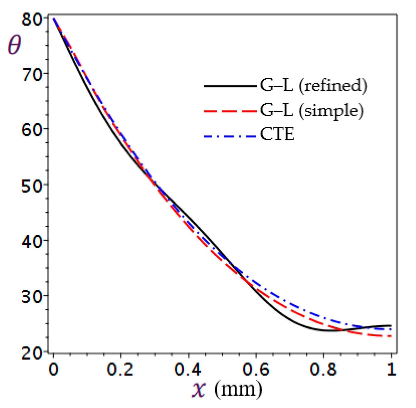
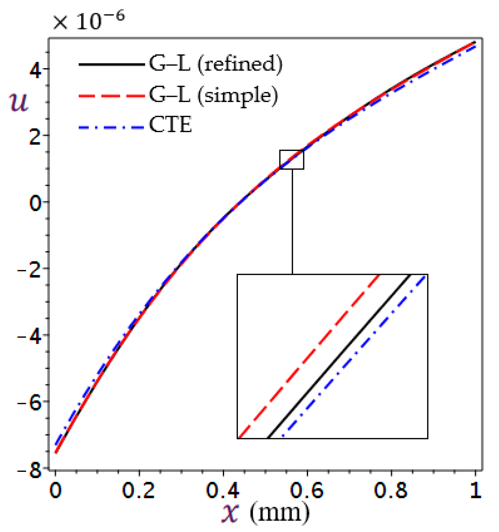
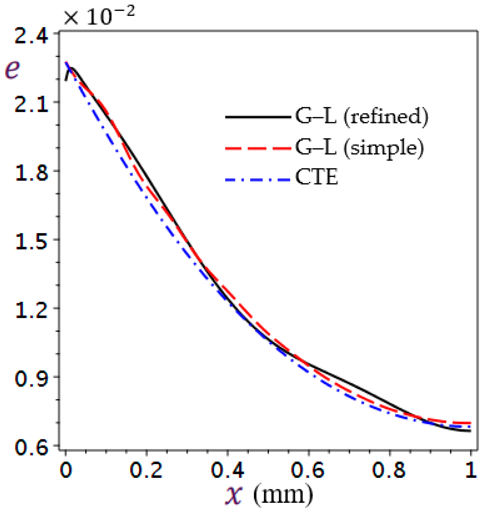
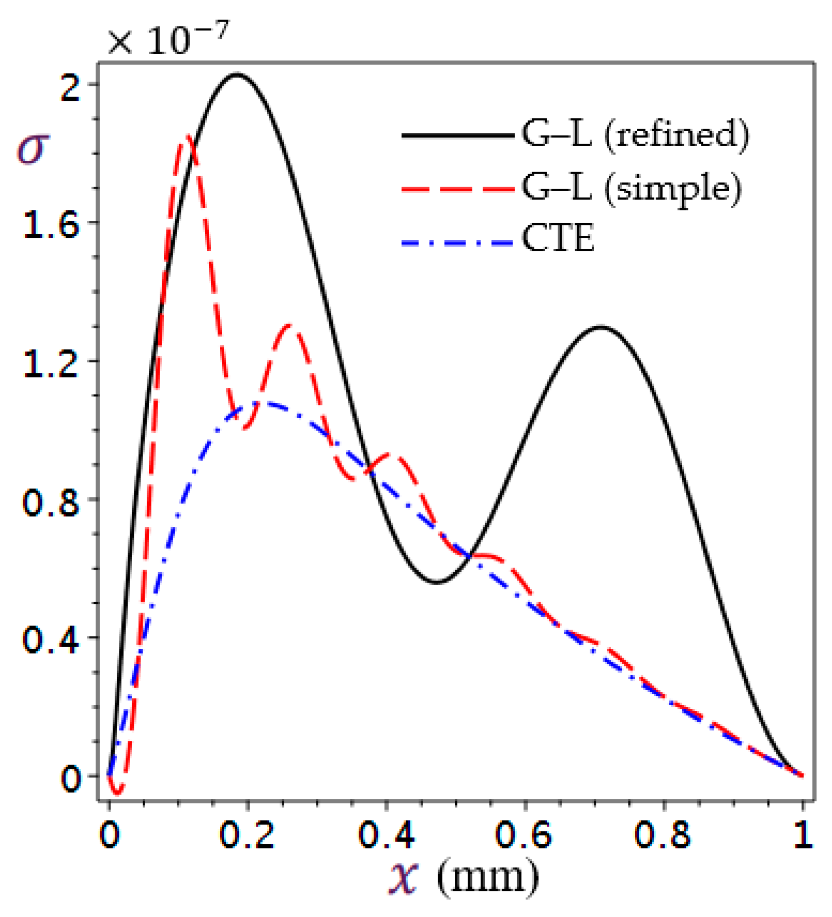
5.1. Validation of Results

The present refined G–L theory is compared with the simple G–L theory as well as the CTE theory. All of them are discussed in Figure 2, Figure 3, Figure 4 and Figure 5. The ramp-type heating parameter is taken by $t_0=9$ s, the time $t=9.1$ s, and the relaxation times are ${\tau }_1=0.3$ s and ${\tau }_2=0.32$ s, satisfying ${\tau }_2\ge {\tau }_1\ge 0$.

In Figure 2, the temperature $\theta$ distributions of all theories show a decrease with the increase in the value of $x$. In addition, it is noticed that the behaviors of the CTE theory and simple G–L theory are similar, while the refined G–L theory takes an oscillatory behavior.

In Figure 3, the displacement $u$ distributions are shown along the $x$-axis. In all theories, the displacement behaves incrementally as the value of x increases. It is also noted that the three theories give displacement very close to each other and that the displacement curve in the refined G–L theory is very close to the one in the simple G–L theory at the edges.

In Figure 4, the distribution of the dilatation $e$ of the three theorems is shown. It is noted that $e$ decreases as the value of $x$ increases. Note also that the dilatation curve in CTE theory is streamlined, while this behavior does not apply to its counterpart in simple G–L theory and refined G–L theory. Where the simple theory fluctuates at the beginning of the skin and then begins to regularize until the curve approaches the curve of the CTE theory, the dilatation curve of the refined G–L theory does not regularize along the x-axis.

Figure 5 shows vanishing values of stress $\sigma$ distributions in CTE, simple G–L, and refined G–L theories at the edges of skin tissues and due to boundary conditions. In addition, in the simple G–L theory, we see that the stress curve has a wave nature, especially from the beginning of the skin to the middle, then the ripple decreases, and the waves become smaller. The same is true in the refined G–L theory but with fewer waves and a behavior that approaches the behavior of the stress curve in the CTE theory.

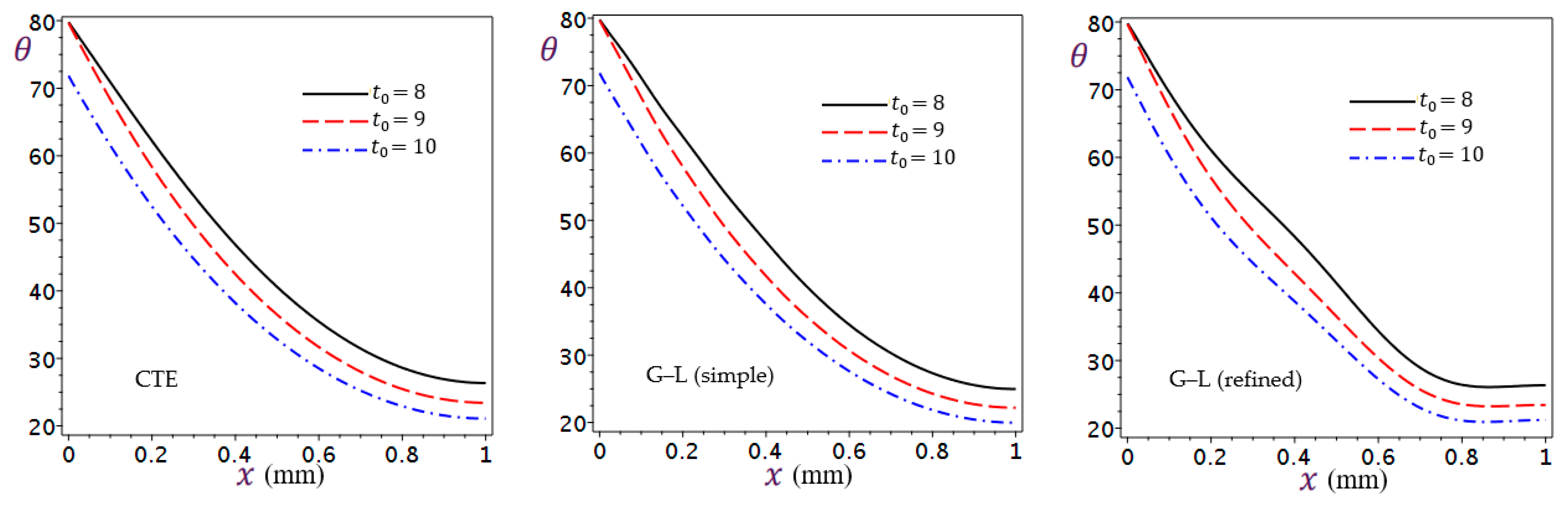
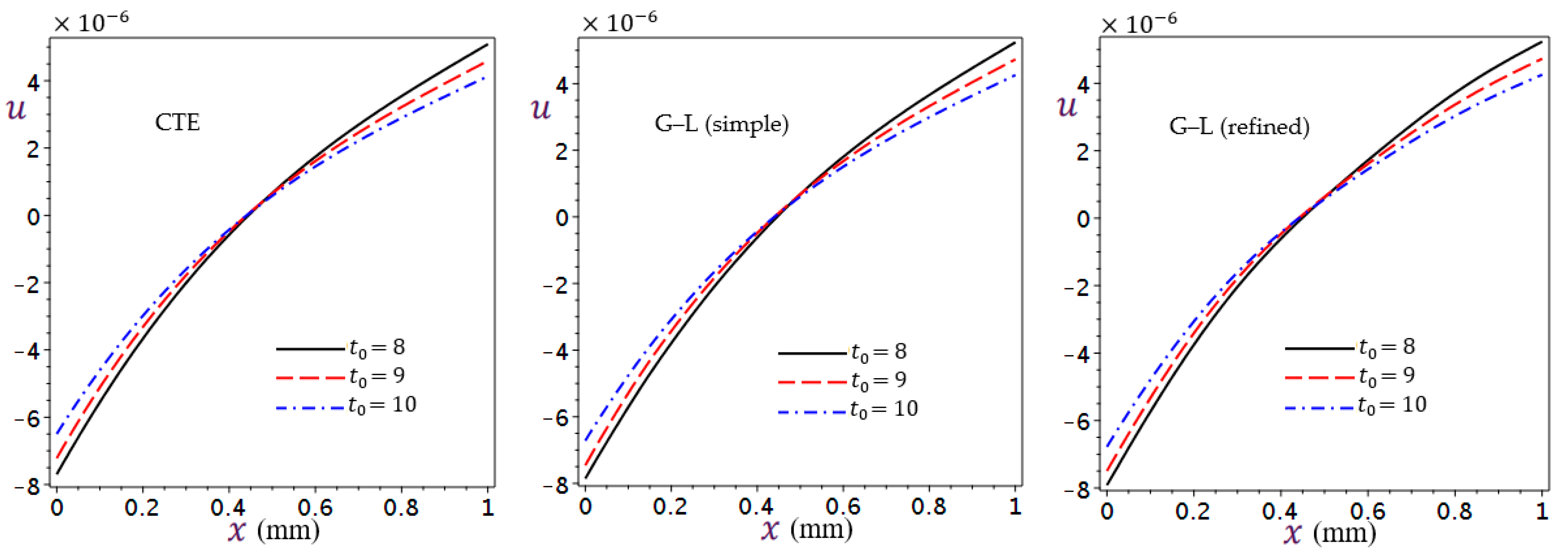
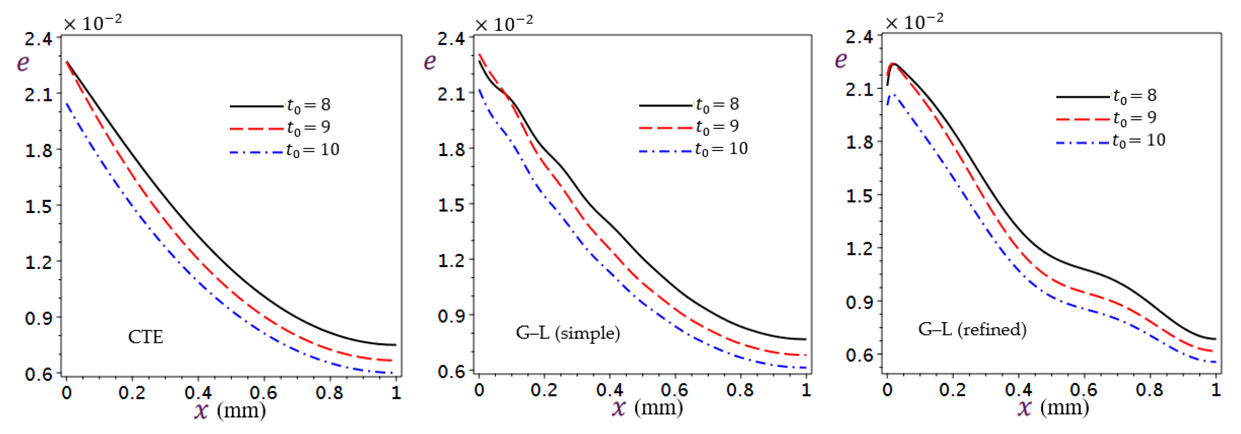
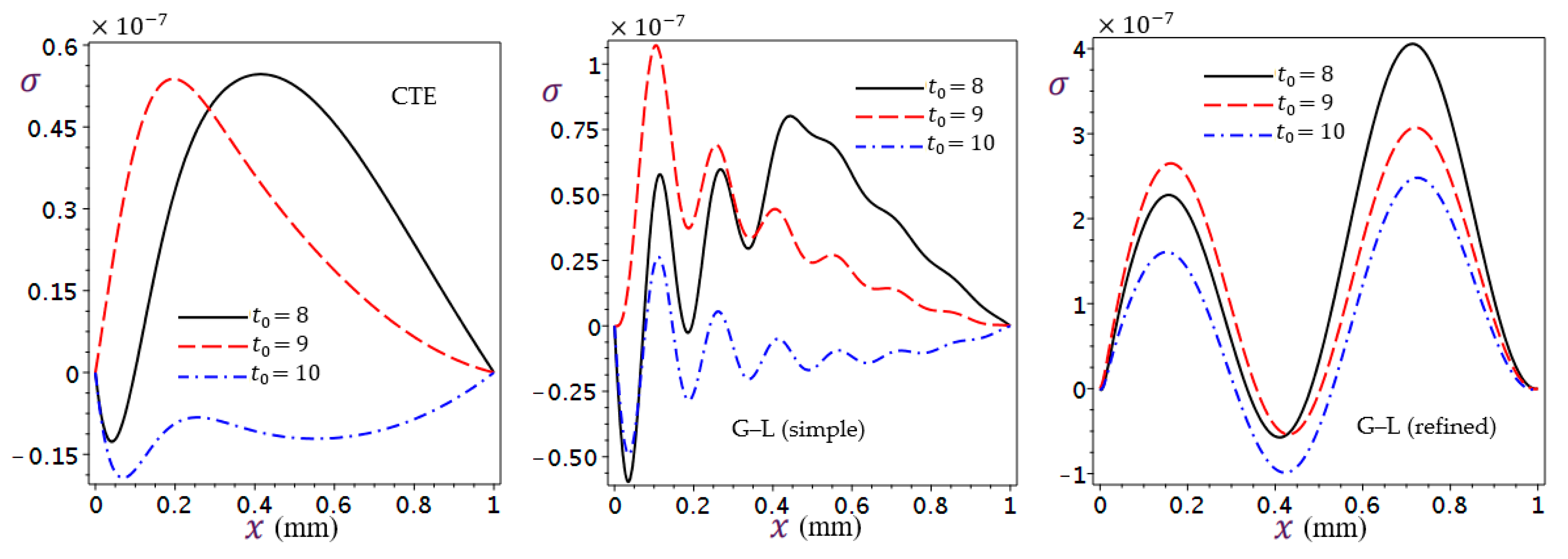
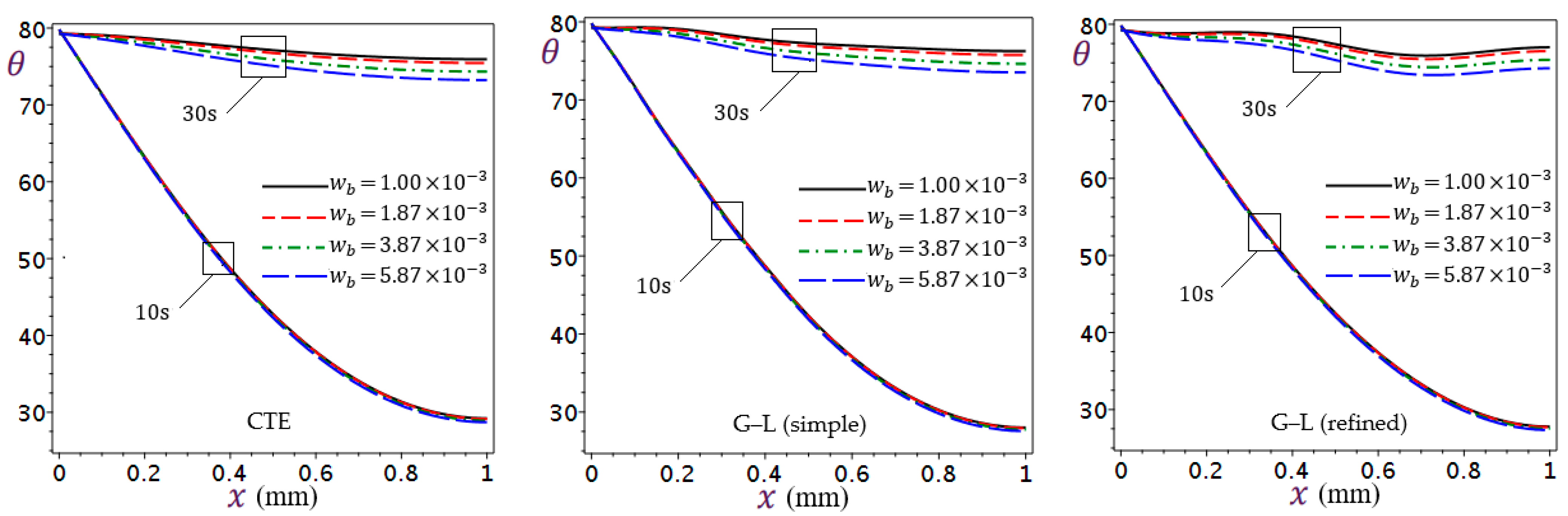
5.2. Effect of Ramp-Type Heating Parameter

Three alternative values of the ramp-type heating parameter were chosen, and the time was fixed by $t=9$ s to represent the distributions of temperature $\theta$, displacement $u$, dilatation $e$, and stress $\sigma$ in the three theories to determine their effects as shown in Figure 6, Figure 7, Figure 8 and Figure 9.

The effect of ramp-type heating parameter $t_0$ on the temperature $\theta$ along the $x$-axis of the skin tissue is shown in Figure 6, where the possible cases of the parameter were studied ($t<t_0$, $t=t_0$ and $t>t_0$). In the three theorems, at position $x=0$, it is seen that when $t\ge t_0$, it satisfies that $\theta \left(0,t\right)={\theta }_0=80$ K in Equation (20), and this comes from the definition of the ramp-type heating function. It is seen that smaller values of the ramp-type heating parameter give higher values of temperature $\theta$ in all theories. The temperature waves of CTE and simple G–L theories have the same behavior. Once again, the refined G–L theory takes an oscillatory behavior after $x=0.2$.

In Figure 7, the effect of the ramp-type heating parameter $t_0$ is shown on the displacement $u$. It is clear that the effect of changing $t_0$ is similar for all theories presented in the above figure, and the displacement vanishes in all theories at $x=0.45$. Before this point, the displacement $u$ increases as the ramp-type heating parameter $t_0$ increases and vice versa after these points.

The effect of the ramp-type heating parameter $t_0$ on the dilatation $e$ along the $x$-axis of the skin tissue is shown in Figure 8. It is shown that the smaller values of $t_0$ give greater values for the dilatation curves in the three theories. The dilatation waves of simple G–L and refined G–L theories have the oscillatory behaviors of $e$ along the $x$-axis, and this is more evident in the refined G–L theory than in the simple G–L theory.

The impact of the ramp-type heating parameter $t_0$ on the normal stress $\sigma$ along $x$-axis of the skin tissue is shown in Figure 9. In the CTE theory, positive stress is obtained when $t=t_0$ and negative stress when $t_0>t$. The stress curves take the same shape in the simple G–L theory when $t=t_0$ and $t<t_0$ with the difference that in the first case the stress takes more positive values than in the second, while when $t>t_0$ the shape of the curve changes. As for the refined G–L theory, the change of $t_0$ does not affect the shape of the stress curve and gives a lower value when $t_0>t$, while in the other two cases ($t=t_0$ and $t<t_0$) the stress curves intersect at $x=0.43,$ and we obtain the highest curve for stress when $t=t_0,$ and the opposite occurs after the intersection.

5.3. Effect of Green–Lindsay Relaxation Times

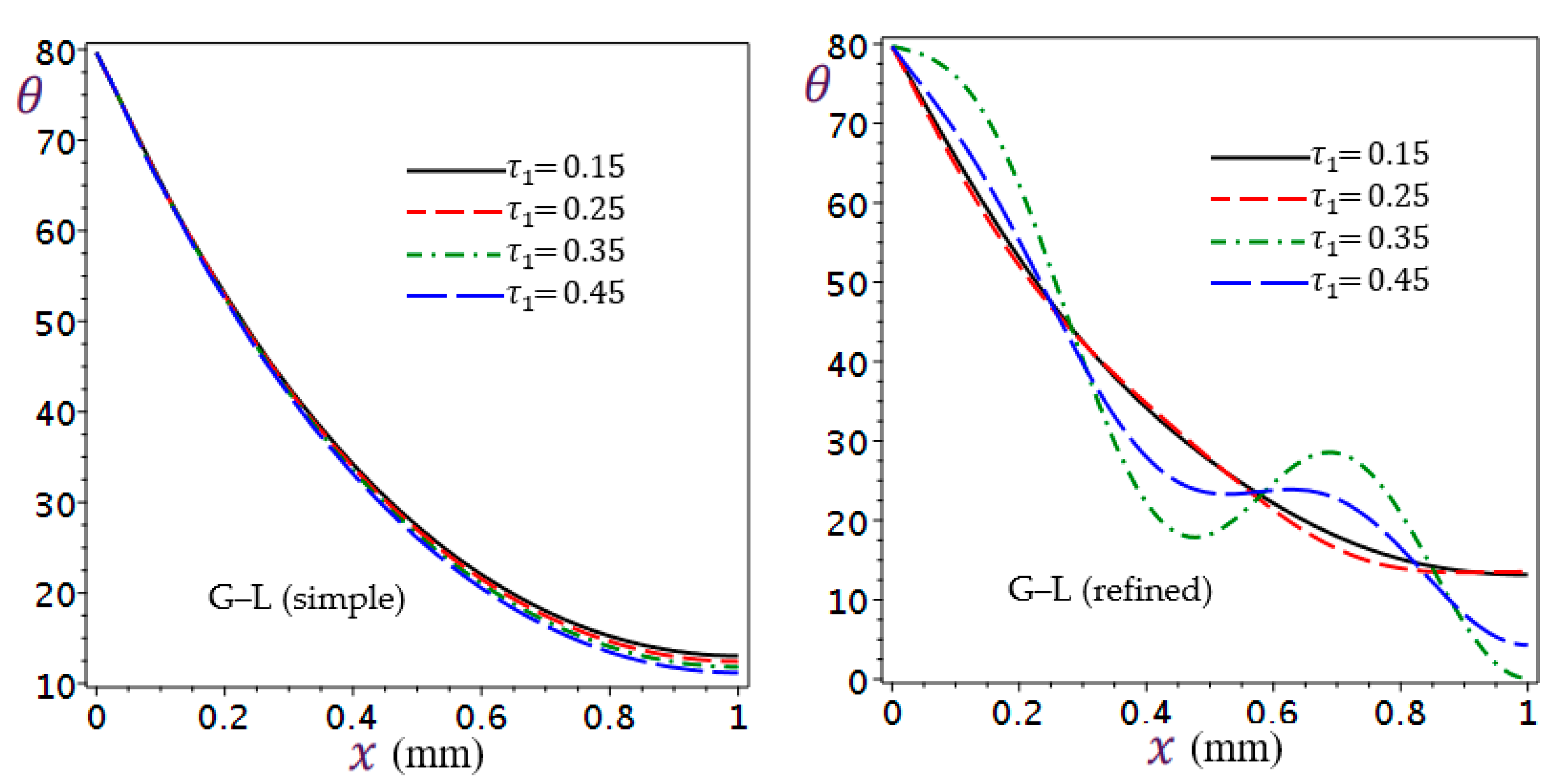
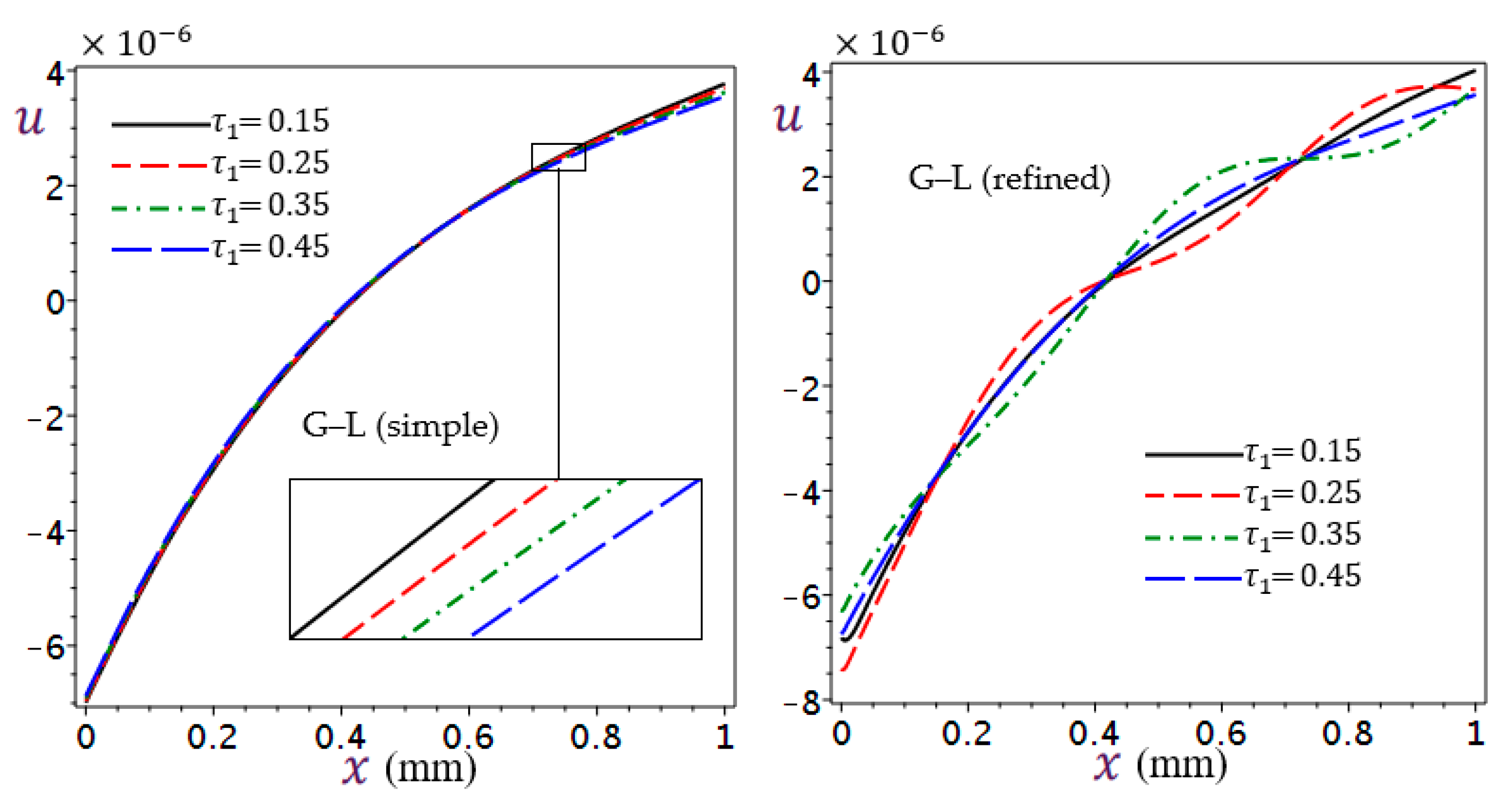
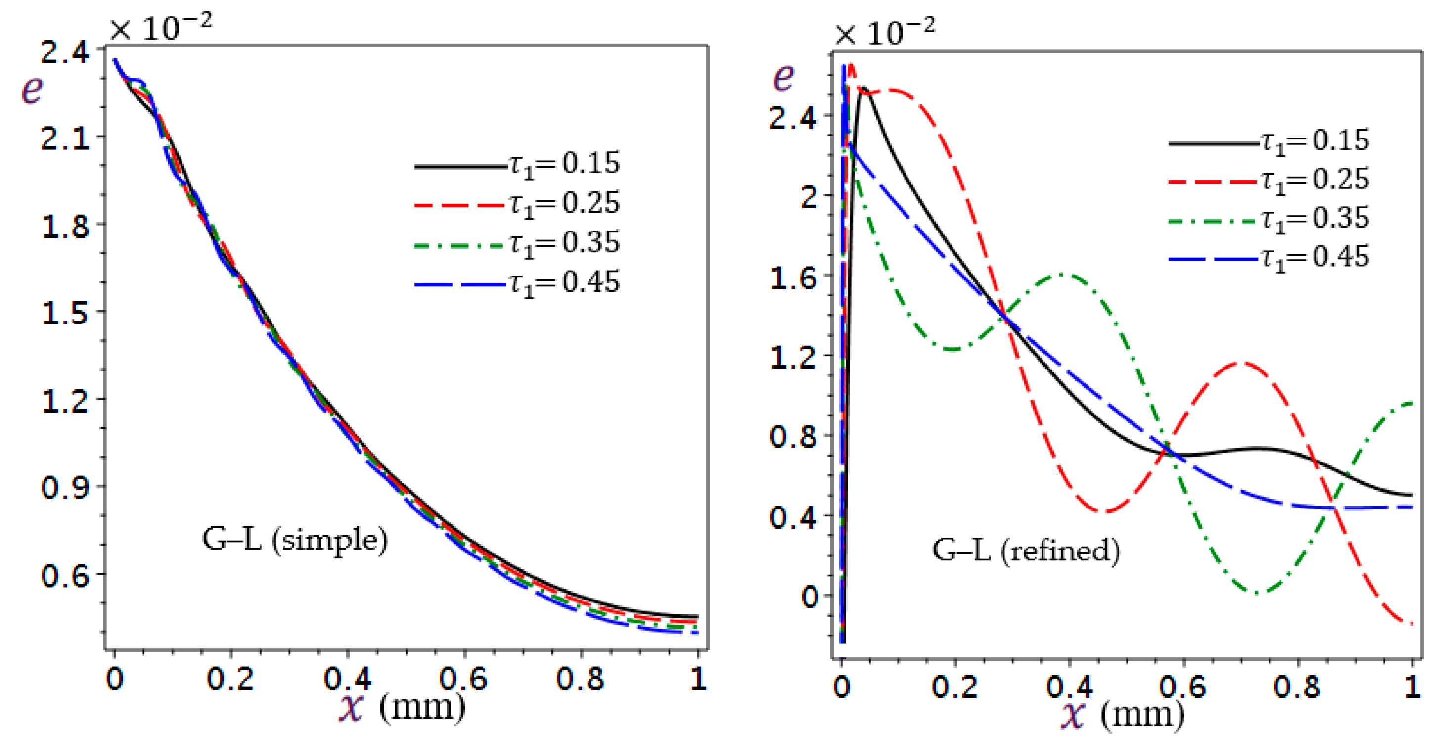
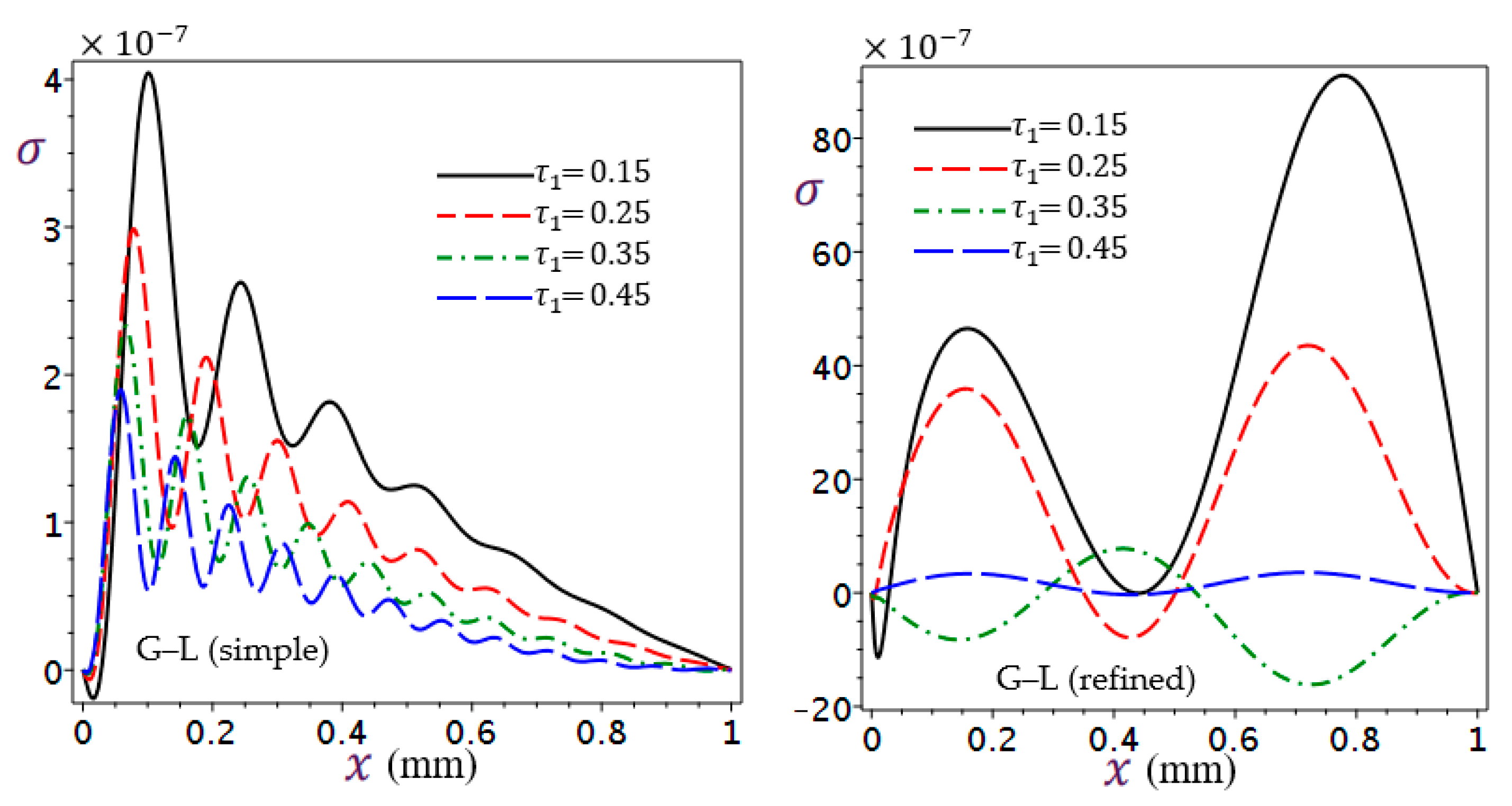
5.3.1. Effect of First Relaxation Time ${\tau }_1$

As shown in Figure 10, Figure 11, Figure 12 and Figure 13, the second relaxation time was fixed at ${\tau }_2=0.5$ s, $t=t_0=6$ s, and four different values for the first relaxation time ${\tau }_1$ are used to investigate its impacts.

Figure 10 shows the effect of the first relaxation time ${\tau }_1$ of the simple and refined G–L theory on the temperature $\theta$. In the simple G–L theory, the temperature curves approach each other, and the values of the greater ${\tau }_1$ give a smaller value of the temperature $\theta$. However, in the refined G-L theory, all temperature curves start from the same point, and then each curve takes on its different behavior; The smaller value of ${\tau }_1$ gives less ripple to the temperature curves, and the heat curve resulting from the larger relaxation times is slower downward than the temperature curves resulting from the smaller relaxation times. From this, we can say that the temperature distribution in the refined G–L theory is more sensitive to the change in ${\tau }_1$ than in the simple G–L theory.

Figure 11 displays the impact of the first relaxation time ${\tau }_1$ of simple and refined G–L thermoelasticity theories on the displacement $u$ of the skin tissue. In this figure, the effect of the variation of the first relaxation time almost vanishes in the displacement $u$ curves as the curves approach each other in simple G–L theory. In the refined theory, the different values of the first relaxation time give different curves from each other. The displacement wave oscillates due to the refined G–L theory with different amplitudes.

Figure 12 shows the effect of the first relaxation time ${\tau }_1$ of the simple and refined G–L theory on dilatation $e$ of the skin tissue. According to this figure, the change in the values of the first relaxation time causes little significant change in the dilatation behavior in the simple G–L theory. However, in the refined G–L theory, the effect of the first relaxation time ${\tau }_1$ on the dilatation is so great that the onset of the curves takes negative values.

Figure 13 shows the effect of the first relaxation time ${\tau }_1$ of the simple and refined G–L theory on the normal stress $\sigma$. Once again, the stress wave starts to oscillate due to the simple G–L theory, noting that the change in ${\tau }_1$ values do not change the shape of the curve of this theory, and the effect is limited to the fact that smaller ${\tau }_1$ give higher stress and vice versa. While the talk differs from the refined G–L theory, where the behavior of the waves differs between each value and another, in this case the smallest value of the relaxation time ${\tau }_1$ is the one that gives greater stress.

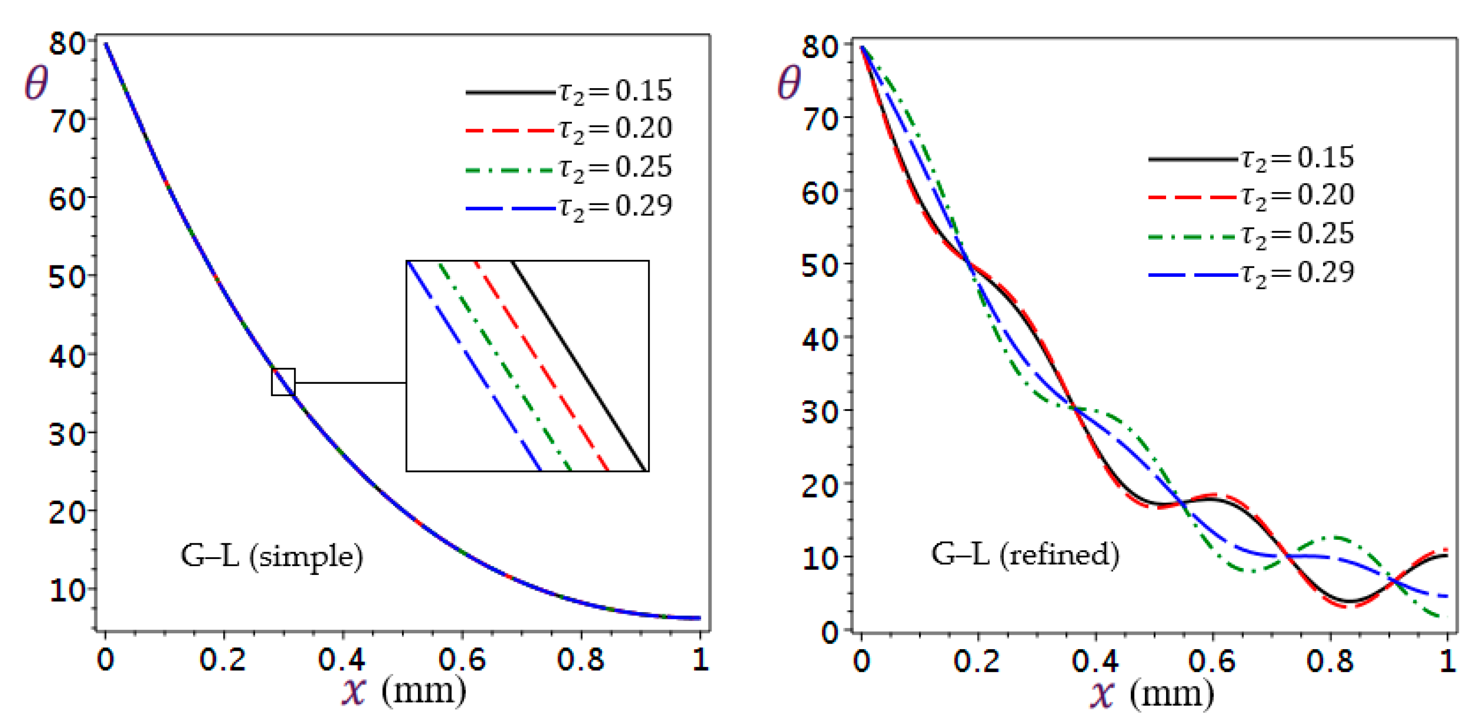
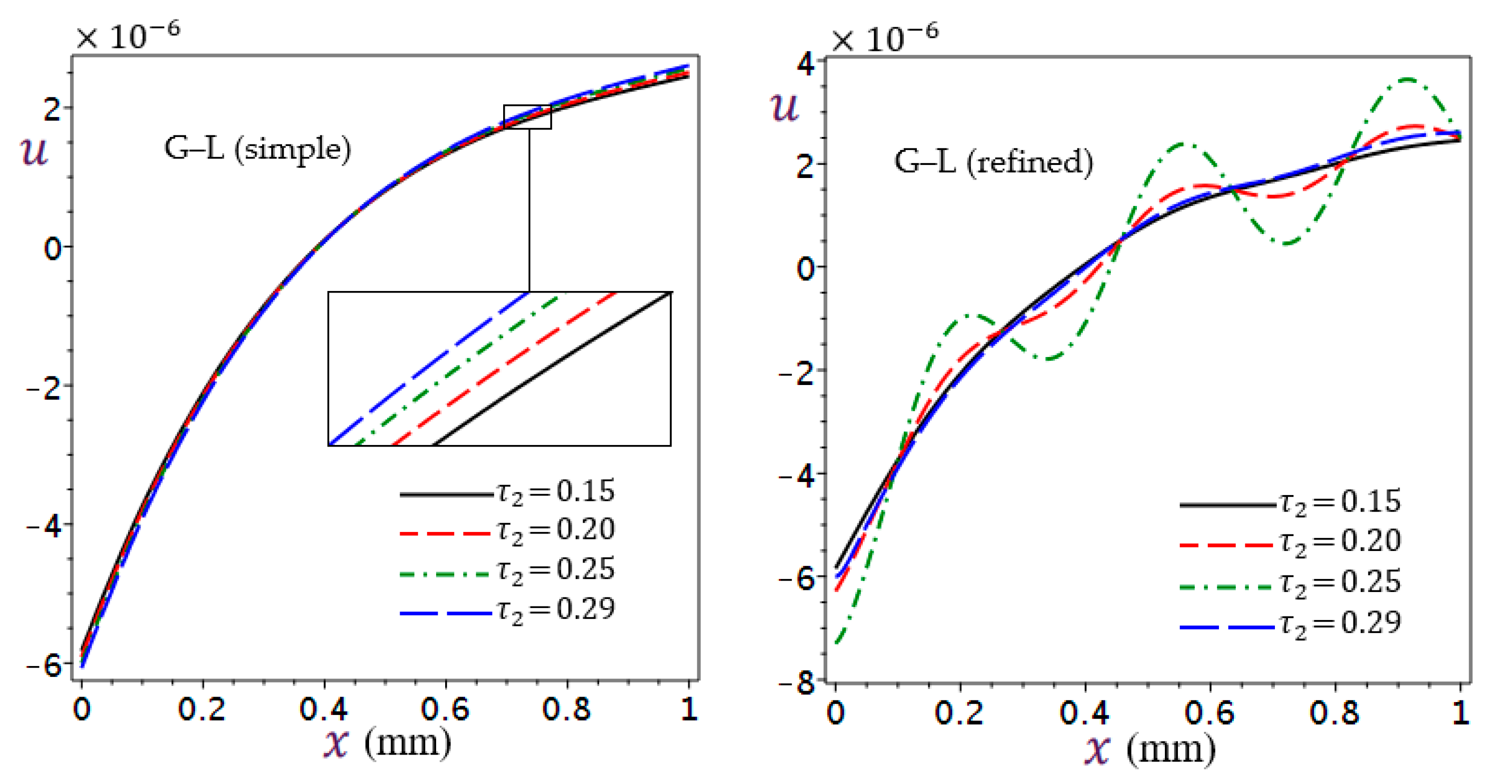
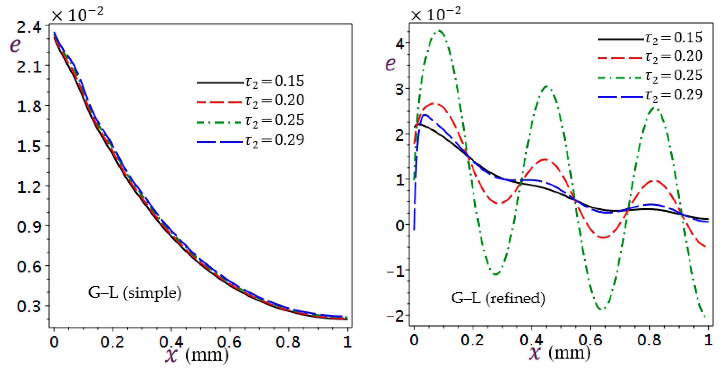
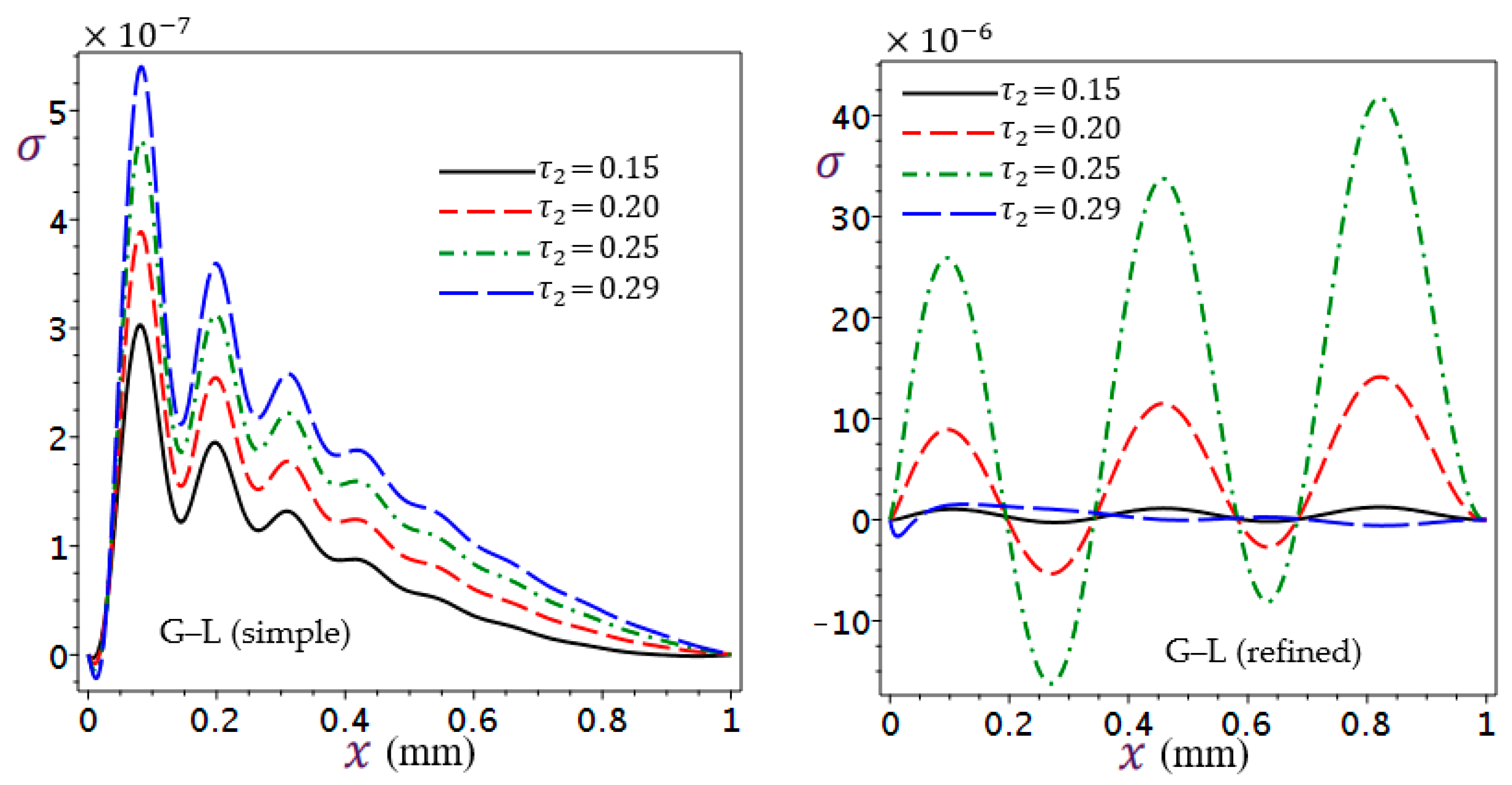
5.3.2. Effect of Second Relaxation Time ${\tau }_2$

To investigate the effect of the second relaxation time of G–L, we fixed the first relaxation time ${\tau }_1=0.1$ s, the time $t=t_0=4$ s, and assigned four different values to the second time, as shown in Figure 14, Figure 15, Figure 16 and Figure 17.

Figure 14 shows the effect of the second relaxation time ${\tau }_2$ of simple and refined G–L theories on the temperature $\theta$ of the skin tissue. It is obvious that the temperature due to the simple G–L theory is not sensitive to the variation of the second relaxation time ${\tau }_2$. When we enlarge some portions, we notice that the temperature increases as ${\tau }_2$ decreases. However, the temperature curves in the refined G–L theory take waves very close to each other at ${\tau }_2=0.15$ s and ${\tau }_2=0.20$ s, but at ${\tau }_2=0.25$ s, the behavior is similar to the first two cases with opposite directions, while the ripple of the curve decreases at the largest value of ${\tau }_2$. This shows that the temperature curve in the refined G–L theory is very sensitive to the variation of the ${\tau }_2$ values.

Figure 15 shows the effect of the second relaxation time ${\tau }_2$ of simple and refined G–L theories on the displacement $u$ of the skin tissue. In the simple G–L theory, the effect of the change in the values of the second relaxation time on the displacement $u$ curve is very small, while the differences in displacement distributions are evident in the refined G–L theory and at ${\tau }_2=0.25$ give a wavier curve. Note that all displacement curves in the refined G–L theory end at the same value at the tip of the living tissue.

Figure 16 shows the effect of the second relaxation time ${\tau }_2$ of simple and refined G–L theories on the dilatation $e$ of the skin tissue. In simple G–L theory, the change in the given ${\tau }_2$ is still small, and the dilatation increases with the increase in the second relaxation time ${\tau }_2$. However, the dilatation curves in the refined G–L theory take on a uniform behavior as waves of equal wavelengths and different amplitudes. This shows that the dilatation curve in the refined G–L theory is super responsive to the changes of the ${\tau }_2$ values.

Figure 17 shows the effect of the second relaxation time ${\tau }_2$ of simple and refined G–L theories on the normal stress $\sigma$ of the skin tissue. The stress waves maintain their shape in the simple G–L theory, and the difference appears because the larger values of ${\tau }_2$ give higher stress. From it and Figure 13, we notice the opposite effect of ${\tau }_1$ and ${\tau }_2$ in the stress distribution in this theory. For the stress curves in the refined G–L theory, the response to the change of ${\tau }_2$ is similar to the response of the dilatation distributions of the same model, where the curve takes the form of waves with different amplitudes, and the ripple of the curve increases with an increase in the value of ${\tau }_2$ and then decreases with the highest given value of ${\tau }_2$.

To demonstrate the effect of the rate of blood perfusion, the temperature distributions were presented in the CTE, simple G–L, and refined G–L theories as in Figure 18, ${\tau }_1=0.3$ s, ${\tau }_2=0.32$ s, and $t_0=9$ s were used. It was noticed that at time $t=10$ s, the influence of the change in $w_b$ appears weak, while the difference appears clear when using a longer time ($t=30$ s), as the increase in the rate of blood perfusion gives less temperature.

Figure 19 shows 3D plots of the temperature $\theta$ distribution along the $x$-axis of the skin tissue due to different theories of thermoelasticity. To be accurate, the temperature $\theta$ distribution in the CTE, simple G–L, and refined G–L theories was shown in three dimensions concerning skin thickness and time changes from $t=8$ s to $t=9$ s with $t_0=9$ s. Through the three cases, it has been observed that the temperature distribution is influenced by the passage of time, as the temperature gives its maximum value at the maximum time, and it is consistent with the condition $\theta =80 \mathrm{K} \mathrm{i}\mathrm{f} t=t_0$. It is also noticed that the shorter time gives a faster ripple of the temperature curve in refined G–L theory, while in the longer times, the curve ripple decreases, and the wave widens.

6. Conclusions

This article presented the Green–Lindsay theory of thermoelasticity in a modified form. It is applied to study the thermoelastic behavior of skin tissue in a one-dimensional under-ramp-type heating. The effect of adding a fourth-order time derivative in addition to the relaxation times of the G–L theory is taken into account. It has been demonstrated that the change affects the distributions of temperature, displacement, dilatation, and stress while preserving the boundary conditions of the problem.

The numerical results showed a decrease in the thermal behavior with the increase in the thickness of the skin because the thermal diffusion of the skin tissue is very low, so the CTE theory and the simple G–L theory took the same shape. The results due to the simple G–L theory were faster in heat dissipation, while those of the refined G–L theory took a fluctuating behavior due to the addition of higher-order time derivatives. The displacement due to the refined G–L theory was similar to those of other thermoelasticity theories, where the displacement behavior increased with increasing the depth of the biological tissue. The behavior of dilatation may be similar to that of the temperature. The behavior of dilatation due to both simple and refined G–L theories is slightly oscillating at the beginning of the skin’s thickness; then the curve becomes smoothy until the dilatation reaches its minimum value at the edge of the skin tissue. Concerning our current theory, the stress resulting from the application of ramp-type heating on the skin takes higher values compared to the rest of the theories of thermoelasticity. This is due to the modification that we made in the stress equation of the current model.

In addition, it is observed that the ramp-type heating parameter affects all three theories (CTE, simple G–L, and refined G–L) in almost the same manner. The lower values of this parameter give high temperature, dilatation, and displacement curves along the tissue. The higher value of the ramp-type heating parameter gives negative stress in the classical and simple theories. However, the effect of this parameter was preserved in the shape of the stress curve of the refined G–L theory, and the change was a regular rise or fall of the curve.

The first relaxation time brings about an appreciable change to the behavior of the curves of all variables in the refined G–L theory, unlike in the simple G–L theory. In addition, the effect of the second relaxation time was more evident in the refined theory than in the simple one.

The effect of the change in blood perfusion on the temperature rates in the three theories appears more clearly after the passage of more time, where the lower the blood perfusion rate, the higher the temperature along the biological tissue. Finally, the change in time had a clear effect on the refined G–L theory more than that in the CTE and simple G–L theories, where the curve took a faster vibratory form with smaller times, and the waves eased with time due to the increase in the difference between time and relaxation times.

Based on the previous results, it can be said that the current model of the refined G–L theory could be useful in the applications of heat transfer through biological tissues, for example, infrared therapy, which depends on the transfer of heat by waves, which contributes to the treatment of many diseases, such as some skin problems such as acne, eczema, and psoriasis, and maintains the freshness of the skin.

References

1. Pennes, H.H. Analysis of tissue and arterial blood temperatures in the resting human forearm. J. Appl. Phys. 1948, 85, 5–34. [Google Scholar] [CrossRef] [PubMed]
2. Tzou, D.Y. The generalized lagging response in small-scale and high-rate heating. Int. J. Heat Mass Transf. 1995, 38, 3231–3240. [Google Scholar] [CrossRef]
3. Biot, M.A. Thermoelasticity and irreversible thermodynamics. J. Appl. Phys. 1956, 27, 240–253. [Google Scholar] [CrossRef]
4. Lord, H.W.; Shulman, Y. A generalized dynamical theory of thermoelasticity. J. Mech. Phys. Solids 1967, 15, 299–309. [Google Scholar] [CrossRef]
5. Green, A.E.; Lindsay, K.A. Thermoelasticity. J. Elast. 1972, 2, 1–7. [Google Scholar] [CrossRef]
6. Mitra, K.; Kumar, S.; Vedavarz, A.; Moallemi, M.K. Experimental evidence of hyperbolic heat conduction in processed meat. ASME J. Heat Transf. 1995, 117, 568–573. [Google Scholar] [CrossRef]
7. Antaki, P.J. New interpretation of non-Fourier heat conduction in processed meat. ASME J. Heat Transf. 2005, 127, 189–193. [Google Scholar] [CrossRef]
8. Liu, K.C.; Lin, C.T. Solution of an inverse heat conduction problem in a bi-layered spherical tissue. Numer. Heat Transf. Part A Appl. 2010, 58, 802–818. [Google Scholar] [CrossRef]
9. Xu, F.; Lu, T.J.; Seffen, K.A. Biothermomechanical behavior of skin tissue. Acta Mech. Sincia 2008, 24, 1–23. [Google Scholar] [CrossRef]
10. Xu, F.; Lu, T.J.; Seffen, K.A.; Ng, E.Y.K. Mathematical modeling of skin bioheat transfer. Appl. Mech. Rev. 2009, 62, 50801–50835. [Google Scholar] [CrossRef]
11. Xu, F.; Seffen, K.A.; Lu, T.J. Non-Fourier analysis of skin biothermomechanics. Int. J. Heat Mass Transf. 2008, 51, 2237–2259. [Google Scholar] [CrossRef]
12. Ng, E.Y.K.; Tan, H.M.; Ooi, E.H. Prediction and parametric analysis of thermal profiles within heated human skin using boundary element method. Philos. Trans. A 2010, 368, 655–678. [Google Scholar] [CrossRef] [PubMed]
13. Kundu, B.; Dewanjee, D. A new method for non-Fourier thermal response in a single layer skin tissue. Case Stud. Therm. Eng. 2015, 5, 79–88. [Google Scholar] [CrossRef] [Green Version]
14. Shih, T.C.; Yuan, P.; Lin, W.L.; Kou, H.S. Analytical analysis of the Pennes bioheat transfer equation with sinusoidal heat flux condition on skin surface. Med. Eng. Phys. 2007, 29, 946–953. [Google Scholar] [CrossRef]
15. Ghazizadeh, H.R.; Azimi, A.; Maerefat, M. An inverse problem to estimate relaxation parameter and order of fractionality in fractional single-phase-lag heat equation. Int. J. Heat Mass Transf. 2012, 55, 2095–2101. [Google Scholar] [CrossRef]
16. Ezzat, M.A.; El-Karamany, A.S. On fractional thermoelasticity. Math. Mech. Solids 2011, 16, 334–346. [Google Scholar] [CrossRef]
17. Jiang, X.Y.; Qi, H.T. Thermal wave model of bioheat transfer with modified Riemann-Liouville fractional derivative. J. Phys. A Math. Theor. 2012, 45, 485101. [Google Scholar] [CrossRef]
18. Ezzat, M.A.; El-Bary, A.A.; Al-Sowayan, N.S. Tissue responses to fractional transient heating with sinusoidal heat flux condition on skin surface. Anim. Sci. J. 2016, 87, 1304–1311. [Google Scholar] [CrossRef] [PubMed]
19. Ezzat, M.A.; El-Karamany, A.S.; El-Bary, A.A. Magneto-thermoelasticity with two fractional order heat transfer. J. Assoc. Arab Univ. Basic Appl. Sci. 2016, 19, 70–79. [Google Scholar] [CrossRef]
20. Kumar, D.; Rai, K.N. Numerical simulation of time fractional dual-phase-lag model of heat transfer within skin tissue during thermal therapy. J. Therm. Biol. 2017, 67, 49–58. [Google Scholar] [CrossRef]
21. Kumar, A.; Shivay, O.N.; Mukhopadhyay, S. Infinite speed behavior of two-temperature Green–Lindsay thermoelasticity theory under temperature-dependent thermal conductivity. J. Appl. Math. Phys. 2019, 70, 26. [Google Scholar] [CrossRef]
22. Chyr, A.; Shynkarenko, H.A. Well-posedness of the Green–Lindsay variational problem of dynamic thermoelasticity. J. Math. Sci. 2017, 226, 11–27. [Google Scholar] [CrossRef]
23. Quintanilla, R. Some qualitative results for a modification of the Green–Lindsay thermoelasticity. Meccanica 2018, 53, 3607–3613. [Google Scholar] [CrossRef]
24. Goudarzi, P.; Azimi, A. Numerical simulation of fractional non-Fourier heat conduction in skin tissue. J. Therm. Biol. 2019, 84, 274–284. [Google Scholar] [CrossRef] [PubMed]
25. Kumar, R.; Vashishth, A.K.; Ghangas, S. Phase-lag effects in skin tissue during transient heating. Int. J. Appl. Mech. Eng. 2019, 24, 603–623. [Google Scholar] [CrossRef] [Green Version]
26. Ezzat, M.A. Fractional thermo-viscoelastic response of biological tissue with variable thermal material properties. J. Therm. Stress. 2020, 43, 1120–1137. [Google Scholar] [CrossRef]
27. Du, B.; Xu, G.; Xue, D.; Wang, J. Fractional thermal wave bio-heat equation based analysis for living biological tissue with non-Fourier Neumann boundary condition in laser pulse heating. Optik 2021, 247, 167811. [Google Scholar] [CrossRef]
28. Youssef, H.M.; Alghamdi, N.A. Modeling of one-dimensional thermoelastic dual-phase-lag skin tissue subjected to different types of thermal loading. Sci. Rep. 2020, 10, 3399. [Google Scholar] [CrossRef] [Green Version]
29. Sobhy, M.; Zenkour, A.M. Refined Lord–Shulman theory for 1D response of skin tissue under ramp-type heat. Materials 2022, 15, 6292. [Google Scholar] [CrossRef] [PubMed]
30. Youssef, H.M.; Salem, R.A. The dual-phase-lag bioheat transfer of a skin tissue subjected to thermo-electrical shock. J. Eng. Therm. Sci. 2022, 2, 114–123. [Google Scholar] [CrossRef]
31. Ezzat, M.A.; Alabdulhadi, M.H. Thermomechanical interactions in viscoelastic skin tissue under different theories. Indian J. Phys. 2023, 97, 47–60. [Google Scholar] [CrossRef]
32. Zhang, Q.; Sun, Y.; Yang, J. Bio-heat response of skin tissue based on three-phase-lag model. Sci. Rep. 2020, 10, 16421. [Google Scholar] [CrossRef] [PubMed]
33. Zhang, Q.; Sun, Y.; Yang, J. Thermoelastic responses of biological tissue under thermal shock based on three phase lag model. Case Stud. Therm. Eng. 2021, 28, 101376. [Google Scholar] [CrossRef]
34. Li, X.Y.; Li, C.L.; Xue, Z.N.; Tian, X. Analytical study of transient thermo-mechanical responses of dual-layer skin tissue with variable thermal material properties. Int. J. Therm. Sci. 2018, 124, 459–466. [Google Scholar] [CrossRef]
35. Shakeriaski, F.; Ghodrat, M.; Escobedo-Diaz, J.; Behnia, M. Modified Green–Lindsay thermoelasticity wave propagation in elastic materials under thermal shocks. J. Comput. Des. Eng. 2020, 8, 36–54. [Google Scholar] [CrossRef]
36. Sarkar, N.; De, S.; Sarkar, N. Modified Green–Lindsay model on the reflection and propagation of thermoelastic plane waves at an isothermal stress-free surface. Indian J. Phys. 2020, 94, 1215–1225. [Google Scholar] [CrossRef]
37. Filopoulos, S.P.; Papathanasiou, T.K.; Markolefas, S.I.; Tsamasphyros, G.J. Generalized thermoelastic models for linear elastic materials with micro-structure Part I: Enhanced Green–Lindsay model. J. Therm. Stress. 2014, 37, 624–641. [Google Scholar] [CrossRef]
38. Zenkour, A.M. Exact coupled solution for photothermal semiconducting beams using a refined multi-phase-lag theory. J. Opt. Laser Technol. 2020, 128, 106233. [Google Scholar] [CrossRef]
39. Zenkour, A.M.; El-Mekawy, H.F. On a multi-phase-lag model of coupled thermoelasticity. Int. Commun. Heat Mass Transf. 2020, 116, 104722. [Google Scholar] [CrossRef]
40. Zenkour, A.M. On generalized three-phase-lag models in photo-thermoelasticity. Int. J. Appl. Mech. 2022, 14, 2250005. [Google Scholar] [CrossRef]
41. Zenkour, A.M.; Mashat, D.S.; Allehaibi, A.M. Thermoelastic coupling response of an unbounded solid with a cylindrical cavity due to a moving heat source. Mathematics 2022, 10, 9. [Google Scholar] [CrossRef]
42. Kutbi, M.A.; Zenkour, A.M. Refined dual-phase-lag Green–Naghdi models for thermoelastic diffusion in an infinite medium. Waves Random Complex Media 2022, 32, 947–967. [Google Scholar] [CrossRef]
43. Zenkour, A.M. Thermal diffusion of an unbounded solid with a spherical cavity via refined three-phase-lag Green–Naghdi models. Indian J. Phys. 2022, 96, 1087–1104. [Google Scholar] [CrossRef]
44. Zenkour, A.M.; Mashat, D.S.; Allehaibi, A.M. Magneto-thermoelastic response in an unbounded medium containing a spherical hole via multi-time-derivative thermoelasticity theories. Materials 2022, 15, 2432. [Google Scholar] [CrossRef] [PubMed]
45. Tzou, D.Y. Experimental support for the lagging behavior in heat propagation. J. Thermophys. Heat Transf. 1995, 9, 686–693. [Google Scholar] [CrossRef]
46. Honig, G.; Hirdes, U. A method for the numerical inversion of the Laplace transform. J. Comput. Appl. Math. 1984, 10, 113–132. [Google Scholar] [CrossRef] [Green Version]
Figure 1. The one-dimensional skin tissue model with boundary conditions.
Mathematics 11 01437 g001
Figure 2. Two-dimensional plots of temperature θ distributions in different theories of thermoelasticity.
Mathematics 11 01437 g002
Figure 3. Two-dimensional plots of displacement u distributions in different theories of thermoelasticity.
Mathematics 11 01437 g003
Figure 4. Two-dimensional plots of dilatation e distributions in different theories of thermoelasticity.
Mathematics 11 01437 g004
Figure 5. Two-dimensional plots of normal stress σ distributions in different theories of thermoelasticity.
Mathematics 11 01437 g005
Figure 6. Effect of ramp-type heating parameter t 0 on temperature θ .
Mathematics 11 01437 g006
Figure 7. Effect of ramp-type heating parameter t 0 on displacement u .
Mathematics 11 01437 g007
Figure 8. Effect of ramp-type heating parameter t 0 on dilatation e .
Mathematics 11 01437 g008
Figure 9. Effect of ramp-type heating parameter t 0 on normal stress σ .
Mathematics 11 01437 g009
Figure 10. Effect of first relaxation time τ 1 of G–L theory on temperature θ .
Mathematics 11 01437 g010
Figure 11. Effect of first relaxation time τ 1 of G–L theory on displacement u .
Mathematics 11 01437 g011
Figure 12. Effect of first relaxation time τ 1 of G–L theory on dilatation e .
Mathematics 11 01437 g012
Figure 13. Effect of first relaxation time τ 1 of G–L theory on normal stress σ .
Mathematics 11 01437 g013
Figure 14. Effect of second relaxation time τ 2 of G–L theory on temperature θ .
Mathematics 11 01437 g014
Figure 15. Effect of second relaxation time τ 2 of G–L theory on displacement u .
Mathematics 11 01437 g015
Figure 16. Effect of second relaxation time τ 2 of G–L theory on dilatation e .
Mathematics 11 01437 g016
Figure 17. Effect of second relaxation time τ 2 of G–L theory on normal stress σ .
Mathematics 11 01437 g017
Figure 18. Effect of rate of blood perfusion parameter w b on temperature θ .
Mathematics 11 01437 g018
Figure 19. Three-dimensional plots of the temperature θ along the x -axis of the skin tissue due to different theories of thermoelasticity.
Mathematics 11 01437 g019
Disclaimer/Publisher’s Note: The statements, opinions and data contained in all publications are solely those of the individual author(s) and contributor(s) and not of MDPI and/or the editor(s). MDPI and/or the editor(s) disclaim responsibility for any injury to people or property resulting from any ideas, methods, instructions or products referred to in the content.