An Efficient Optimization Technique for Training Deep Neural Networks

Abstract

Deep learning is a sub-branch of artificial intelligence that acquires knowledge by training a neural network. It has many applications in the field of banking, automobile industry, agriculture, and healthcare industry. Deep learning has played a significant role in solving complex tasks related to computer vision, such as image classification, natural language processing, and object detection. On the other hand, optimizers also play an intrinsic role in training the deep learning model. Recent studies have proposed many deep learning models, such as VGG, ResNet, DenseNet, and ImageNet. In addition, there are many optimizers such as stochastic gradient descent (SGD), Adam, AdaDelta, Adabelief, and AdaMax. In this study, we have selected those models that require lower hardware requirements and shorter training times, which facilitates the overall training process. We have modified the Adam based optimizers and minimized the cyclic path. We have removed an additional hyper-parameter from RMSProp and observed that the optimizer works with various models. The learning rate is set to minimum and constant. The initial weights are updated after each epoch, which helps to improve the accuracy of the model. We also changed the position of the epsilon in the default Adam optimizer. By changing the position of the epsilon, it accumulates the updating process. We used various models with SGD, Adam, RMSProp, and the proposed optimization technique. The results indicate that the proposed method is effective in achieving the accuracy and works well with the state-of-the-art architectures.

1. Introduction

A convolutional neural network is a type of neural network that was initially invented by researchers to improve image recognition technology. This type of neural network can be trained to recognize patterns in images by identifying the shapes of certain objects or objects in a particular location in the image [1]. When building a convolutional neural network, a dataset consisting of images is required. A neural network is trained to identify certain features in each image in the dataset, which can teach it how to identify the features of other images as well. Once the neural network is trained, it can recognize different objects in new images or identify the locations of those objects in those images [2].

A dense network is a type of neural network that uses multiple layers of neurons to process data. The neurons in a dense network are densely packed, which makes the neural network more efficient at recognizing patterns. These dense networks were first proposed in the 1990s and have seen several improvements over the last few decades, making them more practical for real-world applications [3].

The main difference between a sparse and a “dense” neural network has to do with the number of connections that each neuron in the network has. In a sparse network, each individual neuron in the network is connected to only a few other neurons, whereas in a dense network, each individual neuron is connected to the many other neurons around it. This means that a sparse network typically has fewer connections than a “dense” network, which means that it is less efficient at performing tasks that require processing a large amount of data. On the other hand, a dense network can have more connections than a sparse network, which makes it better at performing tasks such as object recognition and image segmentation [4]. The main advantage of using a “dense” neural network is that it can perform more complex tasks than it can with a “sparse” network.

The major components of a neural network are the input layer, hidden layers, and the output layer. Inputs are received through the input layer, which are then processed and sent through a series of hidden layers and finally to the output layer. Hidden layers store information in the neurons in the layer until a sufficient amount of information has been stored to be processed by the output layer. The output layer then processes the information and sends it back to the user in the form of an answer or prediction [5].

The main advantages of a neural network over other machine learning methods are that it allows for more data to be processed and that it can learn complex relationships between different variables. Neural networks are also more accurate than other methods at classifying data. In addition, neural networks are capable of learning from data and can make predictions without being specifically programmed to do so. Since a neural network is able to learn as it processes information, it can adapt and change as new data becomes available. The ability of a neural network to learn from its mistakes allows it to become more accurate over time and make better predictions [6].

The main objective of any deep learning algorithm is to predict outputs closer to the actual output [7]. It helps to reduce the cost function, which is based on the prediction error. Optimization algorithms play an important role in the forward and backward propagation of a neural network during the training process. It speeds up the training process and finds the optimal parameters for a neural network. An optimization algorithm executes all possible solutions iteratively until it reaches a point that is optimum or satisfactory [8]. Optimal optimizers effectively help neural networks during the training process. Gradient descent is the most basic and popular optimization algorithm. Gradient descent is an optimization algorithm used to minimize some function by iteratively moving in the direction of the steepest descent. There are many variants of the gradient descent optimization algorithm.

Table 1. History of optimizers.

Optimization Algorithms	Pros	Cons	References
Adaptive Gradient	Works well on data with sparse features.	Generalizes worse, converges to sharp minima.	2011 [10]
Adaptive Delta	Keeping the learning rate optimally high.	Accumulation of the squared gradients.	2012 [11]
RMSProp	Works well on data with sparse features.	Generalizes worse, converges to sharp minima.	2012 [12]
SGD with Nesterov Momentum	Accelerates in directions of steady descent. Overcomes weakness of simple SGD	Sensitive to initialization of the learning rate and momentum.	2013 [13]
Adaptive Momentum	Converges faster.	Generalizes poorly.	2015 [14]
AdaMax	Capable of adjusting the learning rate based on data characteristics.	AdaMax tends to overfit very fast.	2015 [14]
Nadam	Nadam uses decaying step size and first momentum hyperparameters to improve the performance.	Generalizes worse, converges to sharp minima.	2016 [15]
AMSGrad	Fixes convergence issues with Adam based optimizers.	Less efficient than AdaDelta and Adam.	2018 [16]
EAdam	Smaller stepsize.	Computationally heavy.l	2020 [17]
EVGO	Requires fewer parameters for tuning.	Generalizes worse, converges to sharp minima.	2020 [18]
LAMB	Less parameters for tuning, faster computation.	Generalizes worse, converges to sharp minima.	2020 [18]
Gravity Optimizer	Faster computation time.	Gradients may vanish due to aggressive scaling.	2021 [19]

includes different types of optimization algorithms in a chronological order. Each optimization algorithm has its own advantages and disadvantages depending on the dataset, computation, implementation, and machine learning model [9].

In this research article, we focus on the different variants of optimization algorithms and aim to introduce a optimization method to improve the accuracy of the machine learning models. The contribution of this paper is as follows:

• We introduce the optimization technique to improve the accuracy of the machine learning model. We have modified the existing Adam optimizer by changing the number of hyper-parameters. The default Adam optimizer utilizes the first hyper-parameter from Momentum and the second hyper-parameter from RMSProp. RMSProp uses an adaptive learning rate, which is why the learning rate changes over time. In this study, we removed the additional hyper-parameter from RMSProp and observed that the optimizer works well without the second hyper-parameter;
• We also changed the position of epsilon in the default Adam optimizer. In the default Adam optimizer, the epsilon is added to the factor after the bias correction step. In the proposed optimization method, the epsilon is added at every step before the bias correction. Due to this it accumulates the updating process;
• We have performed an experiment using open-source datasets such as CIFAR-10 and CIFAR-100. We used machine learning models such as VGG16, ResNet, and DenseNet. We performed a comparison with current state-of-the-art optimizers. During the experiment, we observed that the proposed optimization technique works well as compared to other optimizers.

The rest of the paper is organized as follows. In Section 2, the literature review is described briefly. In Section 3, different variants of the optimization algorithm are explained in detail. In Section 4, different machine learning models used during the experiment are explained. Section 5 includes the proposed methodology. Section 6 exhibits the results achieved during the experiment, and Section 7 concludes the paper.

2. Literature Review

In recent years, deep learning has shown a great impact over the performance of the neural networks in many complicated learning tasks such as natural language processing, image classification, and object detection. A convolutional neural network is a class of artificial neural networks that is used to analyze visual imagery. CNNs have become the state-of-the-art computer vision technique. There are various types of neural networks, such as recurrent neural network (RNN) and convolutional neural network

(CNN) [20,21,22]. CNNs rank best among other neural networks and are widely used for training and testing datasets.

Deep neural networks are standard tool for solving computer vision tasks. Deep neural networks are mostly used for image classification, natural language processing, and rarely for audio recognition. Image classification is one of the most fundamental tasks of computer vision. It has revolutionized and propelled technological advancements in the most prominent fields such as healthcare, banking, automobile industry, and agriculture. Image classification is the process of taking an input, e.g., a picture of a cat or dog, and outputting a class of a picture. Image classification requires a huge dataset. There are many open-source datasets for image classification available online, such as CIFAR-10, CIFAR-100, MNIST, COCO, and ImageNet [23,24,25].

Deep learning is important for the development of artificial intelligence because it allows machines to learn in the same way that humans do [26]. Traditional machine learning methods only rely on information about data that has been specifically programmed into the machine, meaning that it can take a lot of time and effort to train the machine. On the other hand, deep learning allows the machine to learn from its own experiences so that the machine can automatically adapt and learn new information on its own without requiring much human intervention. This capability can accelerate the development of artificial intelligence because it allows the machine to develop its own rules and strategies for problem solving without having to be explicitly programmed to do so. In the future, it may be possible for machines to independently develop their own intelligence without any human assistance at all [27].

There have been various optimizers introduced to train a deep neural network. The majority of deep neural networks use stochastic gradient descent algorithms for better accuracy. SGD can be categorized into two approaches: adaptive learning rate schemes and accelerated schemes. The authors in Ref. [28] proposed a new algorithm named Lookahead. While searching, the algorithm looks ahead at the sequence of ‘fast weights. Lookahead lowers the variance with computation and cost and improves the learning stability. The authors performed an experiment on ImageNet, CIFAR-10/100, and Penn Treebank, and the results showed that Lookahead significantly improved the performance of SGD and Adam.

On the other hand, many deep learning algorithms are used in various fields such as banking, healthcare, automobile industry, and agriculture [29]. Many deep learning algorithms are used in computer vision for object recognition, object detection, and facial recognition. In Ref. [30], the authors used Single Shot Detector (SSD) for object detection in smart homes for security purposes. In the healthcare industry, deep learning algorithms are utilized for the prediction of diseases. In Ref. [31], the authors develop an intelligent model to detect early liver disease. Such models help to diagnose diseases at an early stage and help in the treatment of the disease.

Recently, a lot of research has been conducted for optimizing parameters of deep neural network (DNNs). Gradient-based algorithms are widely used for this purpose. However, there have been issues with parameter optimization, such as vanishing gradients. The authors in Ref. [18] proposed a novel algorithm, named the evolved gradient direction optimizer (EVGO), to cope with the vanishing gradient. The goal of the authors is to find a better search space and modify the gradient value by keeping it away from zero in order to maintain the learning smoothly. The proposed algorithm (EVGO) works by updating the weights of DNNs based on the first-order gradient. The authors also propose a novel hyperplane that makes the gradient better and keeps it close to zero to avoid its position by searching the new space and transferring the properties of the best weight family. The authors perform a comparison with other optimizers such as gradient descent, Adagrad, RMSProp, and Adam. The authors used CIFAR-10/100 and MNIST datasets by using the AlexNet and ResNet architectures. The results indicate that EVGO outperforms the state-of-the-art optimizers and could be used to provide competent momentum in weight updating with the help of the hyperplane to establish robust optimization algorithms.

In Ref. [32], the authors investigate why adaptive optimization methods such as Adagrad, RMSProp, and Adam generalize poorly when compared to SGD. The authors found that adaptive optimization methods perform well in the initial stage of training but SGD outperforms them at later stages of training. The authors observed that Adam could not converge to an optimal solution. The authors introduced an hybrid approach known as ‘Switching Adam to SGD’ (SWATS). The proposed hybrid approach not only solves the convergence problem but also improves the empirical performance. The proposed hybrid approach starts the training with Adam and switches to SGD when appropriate. The authors conduct an experiment on ResNet, DenseNet, and for the CIFAR-10/100 datasets. Their results show that the switching strategy is capable of closing the generalization gap between Adam and SGD.

The authors in Ref. [19] introduce a gravity optimizer for gradient-based optimization. The authors introduce three hyper-parameters and an alternative to the moving average. The gravity optimizer design is based on an inclined plane and using basic kinematic physics. If we consider an inclined plane and a rolling ball, the loss is equivalent to the height of the rolling ball. The authors compare the performance of the gravity optimizer with Adam, RMSProp. The VGGNet model, with a batch size of 128 for 100 epochs, is used for training neural network. The gravity optimizer showed acceptable results and outperformed Adam and RMSProp.

Adaptive based optimization algorithms have witnessed better performance than Adam and RMSProp [14]. Adaptive based optimizations are on the rise and are used in deep learning. Adam is regarded as the default algorithm. There are many variants of the Adam algorithm, such as Adabound, Adabelief, and RAdam. However, the variants perform better than the default Adam algorithm. Variants focus on changing the step size by making differences on the gradient. The authors in Ref. [17] discuss the impact of the constant epsilon. The authors found out that just changing the position of the epsilon will affect the performance of the Adam optimizer. The authors named the algorithm EAdam. EAdam takes a smaller stepsize than Adam. Changing the stepsize makes a significant difference on the gradient. The experimental result indicates that EAdam outperforms Adam and its variants.

Adaptive gradient approaches play an important role in training a deep neural network. Adaptive gradient methods such as AdaGrad, RMSProp, and Adabelief improve the accuracy of the machine learning models by choosing the optimal parameters. The learning rate of such optimizers change to accelerate the training process. Studies show that adaptive learning methods suffer from poor generalization in deep learning tasks. In Ref. [33], the authors propose a novel optimizer (AdaDB) with data-dependent bound on the learning rate. The elements in the learning rate vector is constrained between the dynamic upper bound and constant lower bound. AdaDB is more stable than AdaBound. The experimental results show that the proposed optimizer eliminates the generalization gap between Adam and SGD.

3. Optimization Algorithms

Optimization is an important process in the training of neural networks. The goal of optimization is to find a set of parameters that yields the best performance for a given problem. There are many different methods for performing optimization, each of which has advantages and disadvantages. The most common type of optimization used in neural networks is gradient descent. This method involves repeatedly adjusting the values of the network’s parameters until the performance improves. Different types of problems can be optimized in different ways and by using different methods. In some cases, it is not possible to use gradient descent, which can make it necessary to use another method.

Training a neural network involves setting the parameters of its underlying model such that the network learns to perform the desired task. In order to train a network, it is necessary to define the loss function that will be used to evaluate the network’s performance. A loss function is a function that takes the output of the network and assigns it a numerical value that represents its performance. The values of these parameters must be set so that the network can learn to perform the task well while minimizing the loss function value. The process of adjusting the values of the network’s parameters to minimize the loss is known as the training procedure.

Optimization plays an important role in the training of a neural network. Recent studies have proposed many optimization algorithms. Each optimization algorithm has its own advantages and disadvantages. In this section, we will briefly explain the current state-of-the-art optimizers.

3.1. Stochastic Gradient Descent

There are many different ways to train a neural network and different methods can be useful for different tasks. One of the most common training methods is gradient descent. This method involves adjusting the values of the network’s parameters to minimize the loss function over the course of many iterations. By repeating this process over and over again, the network will learn the weights needed to produce the optimal output for a given input.

There are several important advantages of using gradient descent to train a neural network. First, this method is relatively easy to implement and it is suitable for a wide variety of different problems. Second, it produces high quality results and it performs well even when training large networks with many parameters. Third, it is very easy to optimize for large datasets because it is computationally efficient. Finally, this method is stable and provides a good balance between stability and speed. However, there are also some important drawbacks when using this method. One of the main disadvantages is that it requires a large number of iterations in order to learn the optimal set of parameters. In addition, the performance of this method can degrade when presented with large or complex datasets. There is a higher computational burden on the optimization algorithm when training machine learning models if we have more data points. While updating the gradient descent, all or partial training samples can be taken when calculating the partial derivatives. In gradient descent, whole data is used at once to compute the gradient, whereas in SGD we take a sample while computing the gradient. The gradient descent may not be a good choice if the training sample is too large.

Another approach is to take a part of the data while computing the gradient, which is known as stochastic gradient descent (SGD). In this approach, the learning process proceeds in two phases [34]. In the first phase, the network is initialized with a randomly initialized set of parameters and a loss function is computed over the set of training data. In the second phase, the update procedure is repeated many times until the desired convergence criterion has been met. As in standard gradient descent, the learning process is driven by the minimization of the loss function by alternately updating the weights and the biases of the network. As a result, the method is both stable and scalable and it is also easy to optimize for large datasets. However, an important drawback of this approach is that it requires a large amount of computation time in order to find the optimal set of parameters. For this reason, SGD may not be the best option for all applications.

There are some situations where SGD can become very slow, e.g., when the gradient is consistently small. This is because of the update rule in the algorithms, which only depends on the gradients at each iteration. Noisy gradients can be a problem for SGD as well. To mitigate these issues in neural network training, momentum is used, which can accelerate the gradient descent by taking accounts of previous gradients in the update rule at each iteration. Another method is the Nesterov accelerated gradient. The major difference between the momentum method and Nesterov accelerated gradient is in the gradient computation phase. In the momentum method, the gradient is computed using current parameters, whereas in the Nesterov accelerated gradient, the velocity is applied to the parameters to compute interim parameters. After that, the gradient is computed using the interim parameters [35].

We can use the gradient descent and stochastic gradient descent optimizers separately for the best of both worlds. When using stochastic gradient descent, the neural network is initialized with a set of random parameters and the loss function is computed over a small set of training data. When using gradient descent, the algorithm runs multiple times in order to learn the optimal set of parameters from the full dataset. This approach can be effective for neural network analysis and we can observe which optimizer, i.e., gradient or stochastic gradient descent, is suitable for training the neural networks. The only drawback is that it will require a huge computation time for the analysis.

Stochastic gradient descent is one of the most popular and used optimizers used for deep learning. The main purpose of SGD is to limit the cost work. SGD algorithms are commonly used for huge datasets. Gradient descent utilizes linear regression as given in the following equation.

$$\begin{gathered} W=\omega -\eta ▽Q_i\left(\omega \right) \\ W\leftarrow \eta ▽Q\left(\omega \right) \\ Q\left(\omega \right)=ln\sum i{Q}_i\left(\omega \right)\Rightarrow ▽Q\left(\omega \right)=ln\sum i▽Q_i\left(\omega \right) \end{gathered}$$

(1)

In Equation (1), $\omega$ is the initial weight when training a neural network. $\eta$ is the learning rate at which the parameters are updated. $Q_i$ is the current data being under observation. In general, Q is an error function. SGD computes the best w by minimizing Q. Then, the derivative of the actual and predicted values is taken to find the loss function. W is the updated parameter during the neural network. The last line in Equation (1) represents the error objective with its gradient.

3.2. Adaptive Momentum

Artificial neural networks (ANNs) have come a long way in recent years. First developed in the 1950s, ANNs are now used to process massive amounts of data. They can be used to identify patterns in data and make predictions. Many industries, such as finance, healthcare, and defense, are taking advantage of the power of these machine learning systems. Adam is an algorithm developed by Dr. Hinton at the University of Toronto. It has been used to teach everything from animals to people to machines. It was initially developed for training deep neural networks in machine translation and speech recognition applications. The two main components of Adam are minibatch gradient descent and learning rate schedules. Minibatch gradient descent is a method of calculating the learning rate for individual examples rather than the entire batch. This allows the algorithm to adapt more quickly to changes in the training data. Learning rate schedules are sets of learning rates for different layers in the network. They determine how quickly the network will learn to recognize patterns based on the training data it receives.

Many people are familiar with optimization algorithms such as gradient descent or conjugate gradients. These algorithms are used to find a solution in a given optimization problem. Gradient descent (GD) and conjugate gradients (CG) are iterative algorithms that use local minima as starting points to optimize the objective function. In GD, the steepest descent direction is chosen as the search direction at the beginning of each iteration. In CG, the computed gradient is combined with a conjugate of the Hessian matrix to more accurately determine the steepest descent direction at each iteration.

Both GD and CG have the property that they converge to a local minimum solution. However, GD converges to a local minimum with relatively low cost, while CG converges to a local minimum with relatively high cost. Therefore, these algorithms are not suitable for problems with tight constraints or expensive functions whose optimal solutions lie far away from the current point in the function space.

Recently, Adam optimizer was introduced as an implementation of the gradient-free stochastic optimization method by Kingma and Ba [14]. In this algorithm, both the step size and learning rate are stochastically determined using random sampling from a probability distribution. The step size is controlled by the temperature parameter T and the learning rate is regulated by the RMSprop optimizer. By incorporating these two methods together, the algorithm is able to mimic the dynamics of SGD and use samples from the optimization process to better guide the search towards a better solution. Due to the stochastic nature of the algorithm, it converges more slowly to the optimal solution than SGD and requires more computational resources. In practice, however, the gains achieved by using this method over traditional optimization methods are worthwhile enough to justify the additional computational effort.

The Adam method is one of most efficient and used method based on the GD and momentum. It estimates the adaptive learning rate for all parameters involved in the training of gradients. The mathematical notation for Adam is as follows.

$$\begin{gathered} x_t={\delta }_1\ast x_{t-1}-(1-{\delta }_1)\ast g_t \\ {y}_t={\delta }_2\ast y_{t-1}-(1-{\delta }_2)\ast g_t^2 \\ △{\omega }_t=-\eta \frac{x_t}{\sqrt{y_t+ϵ}}\ast g_t \\ {\omega }_{t+1}={\omega }_t+△{\omega }_t \end{gathered}$$

(2)

In Equation (2), $\eta$ is the learning rate and $g_t$ is the gradient at time t. $x_t$ is the exponential average of gradients along $w_j$. $y_t$ is the exponential average of squares of gradients along $w_j$. ${\delta }_1$ and ${\delta }_2$ are the hyper-parameters. This method has shown superior results over several baseline optimizers in several benchmark tests, including logistic loss regression, linear classification, and logistic regression. For all these tasks, the Adam optimizer produced better final accuracy with smaller training set sizes and fewer iterations compared to conventional optimization methods such as SGD. These results suggest that this algorithm may be a promising alternative to SGD and other traditional optimization methods for a wide range of machine learning applications.

3.3. RMSProp

RMSprop is a technique for reducing the noise in neural networks by smoothing out the errors as they are propagated through the network, but it is unclear how this translates to better network performance when training deep neural networks with hundreds or thousands of layers. In fact, some researchers believe that adding even a single layer of neurons to a deep neural network can reduce the network’s accuracy by up to 10%. However, recent research has shown that using RMSprop can help to reduce this effect and improve the accuracy of deep neural networks [36].

There are two main approaches to reducing the error in deep learning models. The first approach is to reduce the network bias by regularizing it using a loss function that penalizes large values in the network weights. The second approach is to propagate error across the network and smooth out the values in the network weights as much as possible before passing them on to the next layer. This process is known as “weight decay” and is often implemented by adding a small learning rate to the weight updates in every layer. However, adding a regularizer like this can have a detrimental effect on the learning process because the weights do not update quickly as the network learns new information. It can also be challenging to find the right level of regularization, which can make the training of very deep networks very complicated and time-consuming. In contrast, RMSprop does not use a regularizer, so this approach can be less complex and more straightforward to implement in deep learning models.

When training on a set of data, an algorithm goes through a series of processing steps to determine what features are important in the data and the relationships between them. An artificial neural network is a system that mimics this process by using a series of interconnected nodes called “neurons” to process the information. Each neuron takes multiple inputs from the input data and produces an output based on those inputs. The outputs from each neuron are then passed through a series of other neurons to produce the output for the network as a whole. For example, a network trained to recognize images might use a classification algorithm that consists of 3 layers with 10 neurons in each. The output from the first layer would be fed to the second layer as the input, and the output from the second layer would then be passed as input to the third layer. The final output from this third layer would be the network’s prediction about the image being analyzed. The process of updating the weights in the neural network during training helps the network learn to generate accurate predictions based on the input it receives. This process of updating weights is known as “training” or “learning”.

Root Mean Square Propagation (RMSProp) is proposed by Geoffrey Hinton. It is an extension of gradient descent and the AdaGrad that uses a decaying average of partial gradients in the adaptation of the step size for each parameter. In RMS prop, each update is done according to the equation below. The update is done separately for each parameter.

$$\begin{gathered} v_t=\delta \ast v_{t-1}-(1-\delta )\ast g_t^2 \\ △{\omega }_t=-\frac{\eta }{\sqrt{y_t+ϵ}}\ast g_t \\ {\omega }_{t+1}={\omega }_t+△{\omega }_t \end{gathered}$$

(3)

In Equation (3), $\eta$ is the learning rate and $v_t$ is the exponential average of squares of gradients. $g_t$ is the gradient at time t along $w_j$. During training, the weights in the network are updated by changing the values they store for each neuron each time a new batch of training data is received. However, some types of networks are unable to fully adjust their weights and produce inaccurate results during the learning process. This phenomenon is known as “overfitting” since the model has been trained so well on the data that it produces results that are very accurate on that particular set of data but performs poorly when tested on a different set of data. In deep neural networks, this overfitting phenomenon is particularly problematic because the number of parameters in the weight matrix is very large compared to the number of neurons in the network. This can lead to very complex networks with a lot of connections, where changing the weights is often not an effective way to improve the accuracy since the changes are relatively minor compared to the large number of parameters involved.

4. Machine Learning Models

There are different machine learning models such as VGG, ResNet, and DenseNet. We have selected those models in our experiment that require lower hardware requirements and shorter training times compared to their deeper counterparts. Shorter training times allow to test more hyperparameters and facilitates the overall training process. In this section, we will briefly explain the different machine learning models used in this study.

4.1. VGG16

A VGG16 neural network is a 16-layer fully connected artificial intelligence (AI) module. The network was designed as a large-scale feature extractor for use in computer vision and deep learning applications [37]. This deep-learning network performs pixel-wise classification, meaning it assigns each pixel in an image to one of hundreds of categories such as grass, sky, or water. It was inspired by the structure of the visual cortex in the mammalian brain. It consists of millions of artificial neurons that learn to detect patterns by analyzing vast amounts of training data. The training data represent what the network should recognize. For example, if an image of a cat is trained with a cat image, the pixels that represent the cat in the image are labeled as “cat” while the pixels that are outside of the cat are not labeled. Training a network consists of showing it thousands of images until it has learned to recognize those images and the patterns of pixels that they have in common. After training is complete, the network can use the information it has learned about recognizing objects in new images it has not seen before.

VGG16 is a convolution neural network model that achieves 92.7% accuracy in ImageNet. ImageNet is a huge dataset that includes 14 million images of 1000 different classes. It is one of the excellent model architectures. VGG16 has a large number of hyper-parameters that focus on convolution layers of 3 × 3 filter of stride 1 and it always uses the same padding and maxpool layer of 2 × 2 filter of stride 2. The VGG model has two fully connected layers and uses softmax for output. The 16 in VGG16 means that it has 16 layers with weights. It is one of the largest networks, with approximately 138 million parameters.

The VGG network works by passing an input image through the layers of artificial neurons in the network until a single output neuron is reached. Each layer of neurons takes the input from the previous layer and adds its own information about the input image to the information already contained in the previous layer. At the final output layer, a decision is made about whether the input image is a certain category or not. For example, the final layer may label the image of a dog as “dog” or “not dog”. Although the final layer is a binary decision node, it does not actually make decisions directly; instead, it receives input from all the other nodes in the previous layers and combines the information about each image into the final output. The final output is then passed on to the next layer for further processing. As the network continues to make classifications, it becomes more accurate at identifying different objects and begins to sort them into their correct categories. Although the VGG network is specialized for object recognition, other types of neural networks can be used to do many different things, including speech recognition and image processing [38]. For example, an artificial neural network called AlexNet can recognize 1000 different categories of objects, such as “park bench” or “tram”. Neural networks are capable of performing a wide variety of tasks because they can be modified to analyze different types of data and make different predictions based on their training [39].

The training phase of machine learning typically involves feeding the neural network hundreds or thousands of images of particular categories. For each image, the neural network will compare the image to its stored database of images and determine the most likely classification for the image based on the patterns it has previously seen. The more images that the network sees during training, the better it becomes at recognizing objects and distinguishing between similar images. However, some types of data can be harder to train than other types of data. Images are easier to categorize because they have predefined categories that can be labeled easily by humans.

4.2. ResNet50

A ResNet is a type of neural network that was originally designed for object recognition. It is a network of layers, each with multiple neurons. Each neuron in each layer receives information from the previous layer and uses that information to make decisions about how it will affect the information it receives from the next layer. The final layer of the network contains one or more neurons called the output layer. These neurons represent the class or category of the object that is being classified. The network then uses this information to classify the object [40].

ResNet is short form of Residual Network. It is a classic neural network used as a backbone for many computer vision tasks. ResNet50 is a convolutional neural network that is 50 layers deep. The pre-trained network can be used to classify images into 1000 object categories. The network has an image input size of 224 × 224. In our research we used ResNet50, which is a smaller version of ResNet152.

CNN and ResNet are both types of neural networks that are used in computer vision. CNNs and ResNets both use deep learning to identify patterns in an image. However, they differ in how they process images. CNNs are processed line by line, where each line is processed independently. In contrast, ResNets are processed by entire blocks of pixels at a time, which allows patterns to be detected faster and reduces the need to process small sections of the image individually. This results in improved classification accuracy. Another advantage of using a ResNet is that it can handle large amounts of data compared to a CNN.

ResNet can be used to recognize objects in an image. It can also detect faces in images or identify specific objects in an image. It can also be used to detect the orientation of a face in an image, which is useful in facial recognition.

One application of ResNet is for object detection in image and video processing. It can be used to detect objects such as people, cars, animals, etc. Using this method, images can be processed quickly without requiring too many resources. For example, Facebook uses a technique called DeepFace that uses a combination of CNN and ResNet to recognize a person’s face from their profile pictures. Another application is self-driving cars. Self-driving cars use a technique called LiDAR to map their surroundings as they drive. This technique also uses a ResNet to detect and identify objects in its surroundings and avoid collisions. Other applications include medical diagnosis and building security.

4.3. DenseNet121

DenseNet stands for Dense Convolutional Network. It is an architecture that focuses on making the deep learning networks go even deeper. The main feature of DenseNet that makes it unique from other architectures is that it is efficient to train, as it creates shorter connections between the layers. In DenseNet, the first layer is connected with all the other following layers i.e., the first layer, the second layer, and so on. Similarly, the second layer is connected with the third layer, the fourth layer, and so on. This enables maximum information flow between the layers. However, it requires less parameters as compared to a traditional convolutional neural network [41].

Much has been said about the potential of deep learning and its application to various fields such as image recognition, natural language processing, and, more recently, the prediction of future events. By providing an abstract representation of patterns and structures in data, these algorithms can infer useful knowledge from a large amount of data, which would otherwise remain hidden or difficult to interpret. Recently, a deep neural network called DenseNet121, was proposed in a paper published by Stanford University researchers for the task of facial landmark localization in images and achieved state-of-the-art results on the NIST benchmark dataset. This paper investigates the details of this model and its application to the problem of facial landmark localization by comparing it to an existing model known as SSD-101.

Facial landmarks are points on the face that correspond to certain features of the face such as the positions of the eyes, nose, mouth, etc. These points are used to extract other features of the face such as the position, orientation, size, shape, and texture of facial features. As these features can be used to obtain important information about the facial anatomy, which can be used for example to detect disease symptoms or to assist with surgical treatments, it is important to accurately localize facial landmarks so that they can be extracted from images efficiently. The goal of facial landmark localization is to find the points in an image corresponding to those features, which are denoted as facial landmarks. The availability of highly accurate methods for facial landmark localization is therefore important for many applications such as clinical diagnostics, computer animation or virtual reality, and automatic face recognition.

DenseNet121 is a fully convolutional network architecture that is trained on facial landmark datasets from various ethnicities. This model uses a stack of convolution layers followed by several pooling layers and a non-linear activation function to obtain a dense representation of the input image. The final layer of the network predicts the position of the facial landmarks in the image using spatial regression techniques. It is able to achieve state-of-the-art results on the benchmark dataset despite being trained only on a single dataset from a single ethnicity [42].

SSD-101 is a multi-branch deep neural network architecture that consists of three branches: one for extracting local facial feature descriptors from the input image, another for predicting the position of each landmark in the image using spatial regression techniques, and a third branch that combines the output of the first and second branches to produce the final position of each landmark in the image. This method was able to achieve good results when tested on a wide range of benchmark datasets from four different countries but is computationally expensive and difficult to train for large-scale applications.

FaceLoc model was proposed as a solution to the “localization bottleneck” problem in automated facial recognition. This novel method incorporates an appearance model that can encode appearance variations due to age, gender, and lighting condition into the representation learned by the network to improve the ability of subsequent classification steps to identify unknown faces in challenging conditions. It was able to achieve promising results on the various benchmark datasets but cannot be directly used for facial landmark localization because it is designed to perform classification rather than localization tasks. Localization and recognition are the two main components of most face processing systems, and both experience difficult problems and many technical challenges.

5. Proposed Methodology

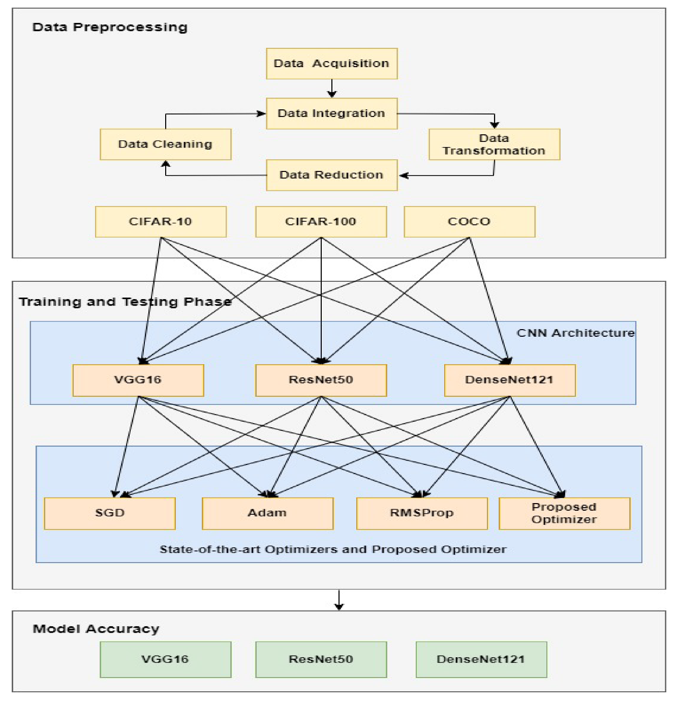
The primary purpose of this work is to develop an optimization technique to improve the accuracy of neural networks. In addition, the optimization technique should reduce the time and complexity of the neural network. In this section, we will briefly explain the proposed methodology. In Figure 1, there are three layers, i.e, the data pre-processing layer, the training and testing phase, and the evaluation of machine learning models. The data pre-processing layer deals with the dataset, the training and testing phase deals with the CNN models and optimizers, and the evaluation phase deals with the model accuracy.

In the data pre-processing layer, we used the CIFAR-10 and CIFAR-100 datasets. The CIFAR-10 and CIFAR-100 datasets are subset of the Tiny Images dataset. The Tiny Images dataset is too large (80 million images) and the images are so small that it can be difficult for people to visually recognize its content. It is one of the most widely used datasets for training machine learning and to compute vision algorithms. The purpose of using the CIFAR-10 and CIFAR-100 datasets is that the images are low-resolution (32 × 32 pixels), due to which we are able to experiment on various models. Data pre-processing is used in machine learning, which refers to the technique for cleaning and organizing the data such that it is suitable for training and testing machine learning models. The CIFAR-10 and CIFAR-100 datasets are available in binary form. We converted the binary form into images. There are 10 classes in the CIFAR-10 dataset and 100 classes in the CIFAR-100 dataset. There are 60,000 images in the CIFAR-10 and CIFAR-100 datasets. In each dataset, 50,000 images are used for training the dataset whereas 10,000 images are used for testing the dataset. In this layer, four steps are performed: firstly, data is integrated, secondly, data is transformed into a usable form, thirdly, the number of input variables is reduced in the training dataset, and lastly, the data is cleaned. Cleaning the data is the process of removing or fixing the corrupt, incorrect formatted data. All the steps involved in the pre-processing phase is for the verification, so that the training of a neural network is smooth.

The training and testing phase includes two parts. In the first part, we selected the current state-of-the-art CNN architectures. In the second part, we selected the current state-of-the-art optimizers and compared it with the proposed optimizer technique. In the training and testing phase, we used different CNN architectures. We used current-state-of-the-art neural networks, i.e., VGG16, ResNet50, and DenseNet121. The details of these CNN architectures is given in Section 4. We used SGD, Adam, and RMSProp. The details of these optimizers is given in Section 3. In the third layer, we evaluate the model accuracy of the selected CNN architectures with various optimizers and the proposed optimizer.

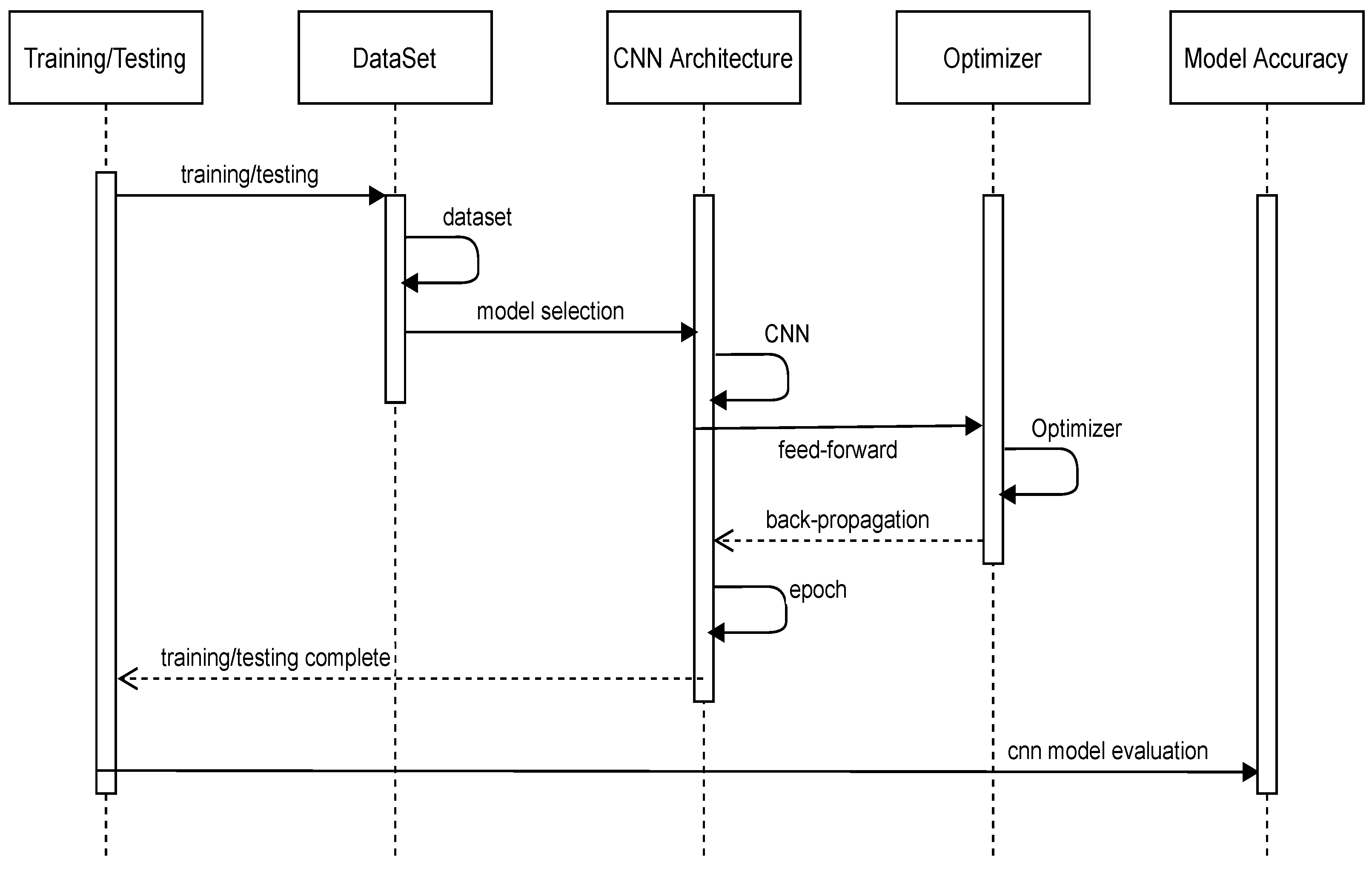
Figure 2 describes the sequence of the proposed optimization technique. There are five phases in the sequence diagram. In this figure, it starts with the training or testing of a neural network. In the first phase, it selects the dataset, i.e., CIFAR-10 or CIFAR-100. The dataset is pre-processed so that it is in a usable format. After selection of the dataset, it selects the CNN architecture, i.e., VGG16, ResNet50, or DenseNet121. We have selected the models in our experiment that require lower hardware requirements and shorter training times compared to their deeper counterparts. Shorter training times allow us to test more hyperparameters and facilitate the overall training process. Finally it selects the optimizer, i.e., SGD, Adam, RMSProp, or Proposed Optimizer. The proposed optimization method is a modified version of the Adam optimizer in which we removed the additional hyper-parameter and also changed the position of the epsilon. After the completion of the training and testing of a neural network, the model is evaluated based on its accuracy. The results show that the proposed optimization method performs well as compared to most of the optimizers.

In deep neural networks, we would like to find the parameters that minimize the loss function. By using those parameters we get the lowest loss on the dataset. In Figure 3, we can see there are local and global minimum points. A local minimum of a function is a point where the function value is smaller than at nearby points, but greater at a distant point. A global minimum is a point where the function is smaller than at all other feasible points. If the loss function is convex, various optimizers such as gradient descent can converge towards global minima, i.e., where the loss value is the lowest. On the other hand, if the function is non-convex, convergence to global minima is not always guaranteed. Due to which, the optimizer may lead towards the local minima convergence, where the loss value is higher than the global minima. More than one local minima can occur in a curve, but there is only one global minima in a curve. The purpose of finding a local and global minima point is to decrease the loss function.

Algorithm 1 is a modified version of the Adam Optimizer. In any optimizer, the learning rate is responsible for alteration of the weights in the neural network concerning the loss gradient. The lower the value, the slower it moves downhill. The reason for keeping a low learning rate is to ensure that the algorithm does not miss the local minimum point. On the other hand, convergence is also proportionally increased. In Algorithm 1, we set the learning rate to 0.001. The learning rate is set to a constant and minimum. In the default Adam Optimizer, there are two hyper-parameters [43]. The Adam utilizes the first hyper-parameter from Momentum and the second hyper-parameter from RMSProp. RMSProp does not treat the learning rate as the hyper-parameter, instead it uses an adaptive learning rate. Due to which the learning rate changes over time in RMSProp [36]. In this study, we removed the additional hyper-parameter from RMSProp because we did not want the learning rate to change over time and observed that the optimizer works well without the second hyper-parameter. In addition, we have modified the position of epsilon in the algorithm. By doing so, epsilon is added to the weights at each step, thus improving the updating process of a neural network. In the default Adam optimizer, the epsilon is added to the factor after the bias correction step. In the proposed optimization method, epsilon is added at every step before the bias correction. Due to which it accumulates through the updating process. Bias-correction gives a better estimate for the moving averages. The difference between EAdam and the proposed optimization method is that in EAdam, the position of epsilon is changed in the default Adam optimizer, whereas in this study, we changed the position of epsilon while removing the additional hyper-parameter in the default Adam optimizer. The change is simple but it requires less computation and hyper-parameter settings. The steps involved in the pseudo-code of the optimization method are as follows.

• $m=0$, first moment vector from Momentum is initialized;
• $t=0$, timestamp is initialized;
• $t=t+1$, update t on each iteration;
• Get the gradients with respect to t;
• Update the first moment vector;
• Epsilon is added at every step before computing the bias;
• Finally update the parameters;
• The loop will continue until the proposed optimization method converges to a solution.

Algorithm 1: Pseudo-code for the proposed optimizer method

1: Learning rate $\partial =0.001$  2: $\beta 1\in [0,1):$ Exponential decay rates for the moment estimates  3: C(w): Cost function with parameters w  4: $w_0$: Initial parameter vector  5: $m_0\leftarrow 0$  6: $i\leftarrow 0$ (Initialize Timestamp)  7: while w not converged do  8:     $i\leftarrow i+1$  9:     $m_i\leftarrow {\beta }_1.m_{i-1}+(1-{\beta }_1).\frac{\partial C}{\partial w}\left(w_i\right)$ 10:     $\widehat{m_i}\leftarrow \frac{m_i}{(1-{\beta }_{1^i})}$ 11:     $w_{i+1}\leftarrow ϵ+w_i-\eta \widehat{m_i}$ 12: end while 13: return $w_i$ (Resulting parameters)

6. Experimental Environment and Results

This section explains the tools and technologies used in implementing and evaluating the proposed optimization technique during the training of neural networks. In this section, we will explain the experimental setup and results obtained during training and testing the deep neural network.

Table 2. Hardware and software details.

Component	Description
System Model	AMD Ryzen 9 5950X
CPU	16-Core Processor 3.4 GHz
GPU	GeForce GT 1030
Operating System	Windows 10
RAM	64 GB
Hard Drive	100TB SSD
Software Tool	PyCharm Professional 2021.12
Programming Language	Python 3.8
Libraries	TensorFlow
Visualizing Tool	TensorBoard

consists of the hardware and software details used during the experiment. We used the AMD based processor with model Ryzen 9. It contained 16-Core Processor with 3.4 GHz. We used a GPU of NVIDIA GeForce GT 1030. For the development we used the Python programming language and PyCharm as a software tool. We used tensorflow libraries for training the deep neural network. Tensorboard is used for visualization process.

Table 3. Summary of the dataset properties.

Dataset	No. of Images	No. of Classes	Images per Class	Image Size	Training Images	Testing Images
CIFAR-10	60,000	10	6000	32 × 32	50,000	10,000
CIFAR-100	60,000	100	600	32 × 32	50,000	10,000

presents the dataset properties used in the experiment. In our experiment, we used the opensource dataset. CIFAR-10 and CIFAR-100 include 60,000 images. Each dataset has 50,000 images for training and 10,000 images for testing the data. In CIFAR-10, there are 10 classes whereas in CIFAR-100 there are 100 classes.

Table 4. Training accuracy for various machine learning models.

Model	Dataset	SGD	Adam	RMSProp	Proposed Method
VGG16	CIFAR-10	97.56	97.77	97.80	97.98
	CIFAR-100	97.60	97.45	97.89	97.50
ResNet50	CIFAR-10	96.25	96.45	96.30	96.89
	CIFAR-100	96.25	96.30	96.45	96.50
DenseNet121	CIFAR-10	97.45	97.45	97.95	97.95
	CIFAR-100	97.20	97.85	97.45	97.85

explains the training accuracy results achieved during the training of the neural network. We used the VGG16 model and CIFAR-10 dataset. We used different optimizers such as SGD, Adam, and RMSProp, and compared the results with the proposed method. The learning rate is set to 0.001, the momentum is set to 0.8, and the weight decay is set to 0.1. The results indicate that the proposed method achieves better training accuracy as compared to the most of the optimizers. Details of the training and testing accuracy are given in Figure 4a. In Figure 4, we used the VGG16 model for training and testing purposes. During the experiment, we used CIFAR-10 and CIFAR-100 datasets. In addition, we used various optimizers and performed a comparison of the proposed optimizer with current state-of-the-art optimizers. During the training process, the proposed optimizer achieved an accuracy of 97.98% whereas during the testing process it achieved an accuracy of 95.95%. We also observed that the training accuracy of the proposed optimization method when using VGG16 model is slightly less than the RMSProp optimizer.

Table 5. Testing accuracy for the various machine learning models.

Model	Dataset	SGD	Adam	RMSProp	Proposed Method
VGG16	CIFAR-10	95.45	95.89	95.54	95.95
	CIFAR-100	95.30	95.10	95.55	95.60
ResNet50	CIFAR-10	94.40	94.60	94.70	94.80
	CIFAR-100	94.10	94.50	94.40	94.60
DenseNet121	CIFAR-10	95.10	95.70	95.20	95.80
	CIFAR-100	95.00	95.20	95.40	95.50

explains the testing accuracy results achieved during the testing of the neural network. We used the VGG16 model and CIFAR-10 dataset. We used different optimizers such as SGD, Adam, and RMSProp, and compared the results with the proposed method. The results indicate that the proposed method achieves better training and testing accuracy as compared to most of the optimizers. Details of the training and testing accuracy are given in Figure 4.

Figure 5 shows the performance of the ResNet50 model for training and testing purposes. During the experiment, we used CIFAR-10 and CIFAR-100 datasets. In addition, we used various optimizers and performed a comparison of the proposed optimizer with current state-of-the-art optimizers.

Figure 6 shows the performance of the DenseNet121 model for training and testing purposes. During the experiment, we used CIFAR-10 and CIFAR-100 datasets. In addition, we used various optimizers and performed a comparison of the proposed optimizer with current state-of-the-art optimizers.

7. Analysis and Discussion of the Results

In this section, we will discuss various performance metrics used during the training, validation, and testing phase of the different models. We will compare the results of each model and evaluate their performance.

Performance Metrics

Accuracy, precision, recall, and f-measure are all measures of the closeness of a result to the true value. Accuracy measures how close the result is to the true value. Equation (4) is the formula used to calculate the accuracy. In Figure 7, DenseNet121 has higher accuracy during the training as compared to other models, i.e., VGG16 and ResNet50. Whereas during testing, VGG16 has higher accuracy as compared to other models.

$$Accuracy=\frac{TP+PN}{TP+PN+FP+FN}$$

(4)

Precision measures how often the results are within a certain range. Precision can be thought of as the number of correct results divided by the total number of possible results. Equation (5) is used to calculate precision. In Figure 7, DenseNet121 has a higher precision value as compared to other models during the training and testing phase.

$$Precision=\frac{TP}{TP+FP}$$

(5)

Recall can be thought of as the percentage of results that are correct divided by the total number of results that the model predicts. Equation (6) is used to calculate the recall. DenseNet121 has a higher recall value as compared to other models during the training and testing phase.

$$Recall=\frac{TP}{TP+FN}$$

(6)

Specificity itself can be described as the algorithm/model’s ability to predict a true negative of each category available. Equation (7) is used to calculate specificity. VGG16 has a higher specificity value as compared to other models during the training and testing phase.

$$Specificity=\frac{TN}{TN+FP}$$

(7)

F-measure is a measure of the accuracy of a model’s predictions in relation to its complexity. The higher the F-measure, the better the model is performing (F = F1 + F2). An accuracy of 100% means that the model is perfectly accurate. Equation (8) is used to calculate the F-measure. ResNet50 has a higher F-measure value as compared to other models during the training and testing phase.

$$F-measure=\frac{2\ast Precision\ast Recall}{Precision+Recall}$$

(8)

Figure 8 shows the training and validation loss of the various models used with the proposed optimization methods. During the experiment, we used the CIFAR-100 dataset. Training loss is a metric used to assess how a deep learning model fits the training data. The error of the model is assessed on the training set. It is calculated by taking the sum of errors, for each example in the training set.

On the other hand, validation loss is a metric used to assess the performance of the deep learning model on the validation set. The validation set is a portion of the dataset used to validate the performance of the model. It is calculated by taking the sum of errors for each example in the validation set.

If the validation loss is greater than the training loss, it indicates that the model is underfitting. It occurs when the model is unable to train data accurately and generates errors. If the validation loss is greater than the training loss and changes frequently, it is known as overfitting. This model is not trained accurately and cannot generalize on new data. The model performs well on training data but poorly on new data. In overfitting, the validation loss decreases at some point but starts to increase again. If the training and validation loss both decrease and stabilize at a specific point, it indicates an optimal fit. It means that the model is well trained and does not overfit or underfit. In Figure 8, we can see that all the curves are at an optimal fit while using various models with the proposed optimization method.

A limitation of the present work is that only two openly available datasets were used. As a consequence, an overfitting with a lower generalizability of the results cannot be excluded and should be considered when interpreting our results. However, this is a common problem in deep learning research.

8. Conclusions

In this study, we aim to improve the optimization technique for training deep neural networks. Deep learning plays a major role in computer vision tasks such as image classification, natural language processing, and object detection. During deep neural network training, optimizers play an important role in improving the accuracy and reducing the training time. Optimizers are algorithms that are used to maximize the efficiency of the model or minimize the loss function. Recent studies have proposed many state-of-the-art optimizers to support the neural network training. Each optimizers has its own advantages and disadvantages. In this study, we focus on different variants of optimization techniques and aim to introduce a optimization method to improve the accuracy of the deep neural networks. We conducted an experiment using the VGG16, ResNet, and DenseNet model with the CIFAR-10 and CIFAR-100 datasets. We have made some modifications in the Adam optimizer by minimizing the cyclic path in the algorithm, removing the additional hyper-parameter, and changing the position of the epsilon. We used SGD, Adam, and RMSProp optimizers and compared the training and testing accuracy with the proposed optimization method. As shown in Section 6, the proposed methodology outperforms the current-state-of-the-art optimizers with a marginal improved accuracy. During the training process, the proposed optimizer achieved an accuracy of 97.98%, whereas during the testing process it achieved an accuracy of 95.95%. We also observed that the training accuracy of the proposed optimization method when using VGG16 model is slightly less than the RMSProp optimizer. To conclude, the overall results indicate that the proposed method is effective in achieving the accuracy and works well with the current architectures.