Article

Predicting the Future Appearances of Lost Children for Information Forensics with Adaptive Discriminator-Based FLM GAN

1
Department of Computer Science and Engineering, Swami Vivekananda Institute of Science & Technology, Kolkata 700145, West Bengal, India
2
Amity Institute of Information Technology, Amity University, Kolkata 700135, West Bengal, India
3
Department of Information Technology, Maulana Abul Kalam Azad University of Technology, West Bengal, Haringhata 741249, West Bengal, India
4
Department of Computer Science and Engineering, Sikkim Manipal Institute of Technology, Majitar 737136, Sikkim, India
5
Department of Environmental Health, Harvard T. H. Chan School of Public Health, Boston, MA 02115, USA
6
Department of Pharmacology & Toxicology, The University of Arizona, Tucson, AZ 85721, USA
7
Department of Computer Science and Engineering, Maulana Abul Kalam Azad University of Technology, West Bengal, Haringhata 741249, West Bengal, India
*
Author to whom correspondence should be addressed.
Mathematics 2023, 11(6), 1345; https://doi.org/10.3390/math11061345
Submission received: 23 January 2023 / Revised: 1 March 2023 / Accepted: 6 March 2023 / Published: 10 March 2023
(This article belongs to the Section Mathematical Biology)

Abstract

:
This article proposes an adaptive discriminator-based GAN (generative adversarial network) model architecture with different scaling and augmentation policies to investigate and identify the cases of lost children even after several years (as human facial morphology changes after specific years). Uniform probability distribution with combined random and auto augmentation techniques to generate the future appearance of lost children’s faces are analyzed. X-flip and rotation are applied periodically during the pixel blitting to improve pixel-level accuracy. With an anisotropic scaling, the images were generated by the generator. Bilinear interpolation was carried out during up-sampling by setting the padding reflection during geometric transformation. The four nearest data points used to estimate such interpolation at a new point during Bilinear interpolation. The color transformation applied with the Luma flip on the rotation matrices spread log-normally for saturation. The luma-flip components use brightness and color information of each pixel as chrominance. The various scaling and modifications, combined with the StyleGan ADA architecture, were implemented using NVIDIA V100 GPU. The FLM method yields a BRISQUE score of between 10 and 30. The article uses MSE, RMSE, PSNR, and SSMIM parameters to compare with the state-of-the-art models. Using the Universal Quality Index (UQI), FLM model-generated output maintains a high quality. The proposed model obtains ERGAS (12 k–23 k), SCC (0.001–0.005), RASE (1 k–4 k), SAM (0.2–0.5), and VIFP (0.02–0.09) overall scores.
MSC:
68T07

1. Introduction

This article aims to show a deep learning-based investigation method for missing children’s cases. A breach of the law in disappearing children cases increases the risks of exploitation through criminal activity. A detailed description of the lost children, recorded through the initial investigation, leads to failure as after a few years, the missing children’s faces start to change with aging. Our method tries to predict the aging effect while presenting the personalized attributes of the children’s faces. The supervised-based DNN explored in this literature requires a range of faces of a similar object for a long time to perform training. In recent years, GAN and its variant (viz., cGAN) achieved poor performance compared to physical and prototype-based methods [1,2,3] to train the facial aging method with solitary data. The Tufts [4] face dataset are used to evaluate the performance of the proposed work. cGans-based [5,6,7,8] approaches fail to achieve the demands for picture quality (i.e., aging precision and identity retention) while training the network to understand the effects of aging between the two rare age groups.
On the contrary, GAN tries to increase the performance by loading facial attribute vectors into the generator and discriminator by presenting the congruent face characteristics. Therefore, these works offer a StyleGan ADA [1] based framework to generate the prediction. The StyleGan ADA feed discriminator with information about the type of errors produced by generator. The statistical evaluation of activation function performs real and model generated data identification through feature matching. The proposed approach was tested with multiple hyperparameters using the KinFaceW dataset. The best accuracy was achieved with F1L2M8 hyperparameter, where F1 represents the feature map as 1×, L2 is the learning rate set to 2 and M8 as 8 parameter mapping net depth. F1L2M8 obtains a 10–30 BRISQUE score for the image quality using KinFaceW-I and KinFaceW-II datasets. The model-generated outputs obtain MSE (2 k–5 k), RMSE (4–7), PSNR (10–14), SSIM (0.2–0.5), UQI (0.7–0.8), and MSSSIM (0.2–0.5).

2. Related Works

A latent distribution strategy using generator mapping was implemented by Fokker Plank [9] in the data space. It includes a plug-and-play facility to use directly the pre-trained GAN [10] models. The article consists of several rigorous experiments on the complex data distribution. It has Wasserstein gradient flow with the convexity of the f-divergence method [11] that preserves informational identity by evaluating applicability for structural correspondence. The following approach utilizes the FRGS-V2 dataset to generate real-life application scenarios. We compare the results with the MAD and SOTA procedures. To maintain robust and accurate performance, MIPGAN [11] applies Arcface. MIPGAN [11] Combined few pre-trained GAN architectures to produce images maintaining perceptual quality metrics. MIPGAN minimizes binary cross entropy loss by balancing inner product between real and generated samples. This GAN framework avoid generation of unrealistic samples from distance-based objectives. The generated data are re-digitized for morphing attack detection mechanisms. Applying deformation via prints or lines controls the image curves in MLS [12]. In [12], it implements the slightest square deformation to produce a linear system from partial derivatives of the plotted matrix. MLS represents affine deformation for stretching the result. Uniform scaling is updated with similarity deformation to learn from observations. Rigid deformation iterates eigenvalue and vectors for covariance evaluation. In Automatic Interpolation and Recognition (AIRF) [13], new views are generated via linearly interpolated fields of the given input. This evaluation mechanism uses Gaussian probability distribution for approximation. AFR [14] applies discrete cosine transformation to classify featured vectors. It combines Benford features with the linear support vector machine as the classifier. [15] proposed a distribution scale-specific latent factor variation to quantify disentanglement.

3. Major Contribution

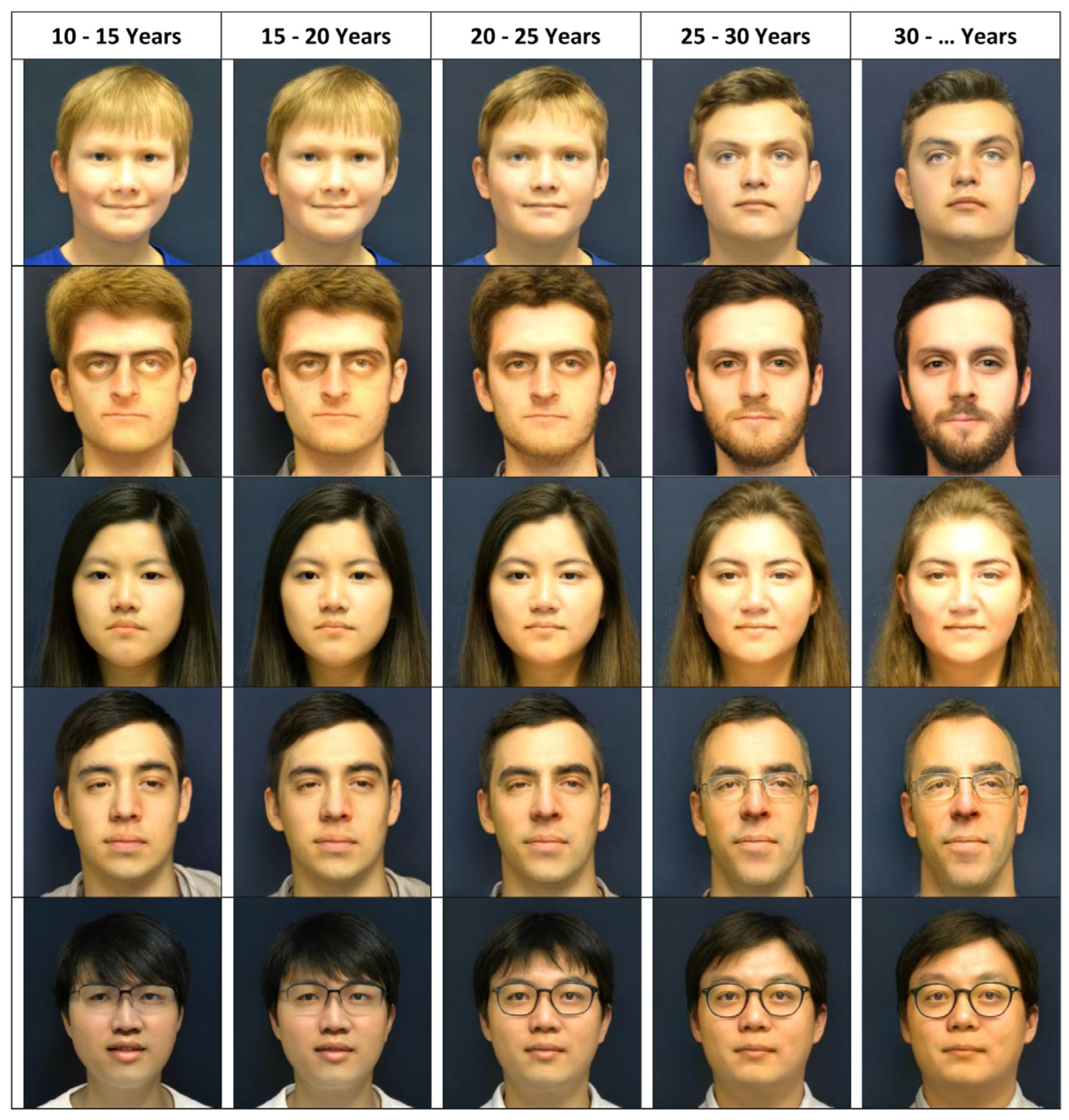
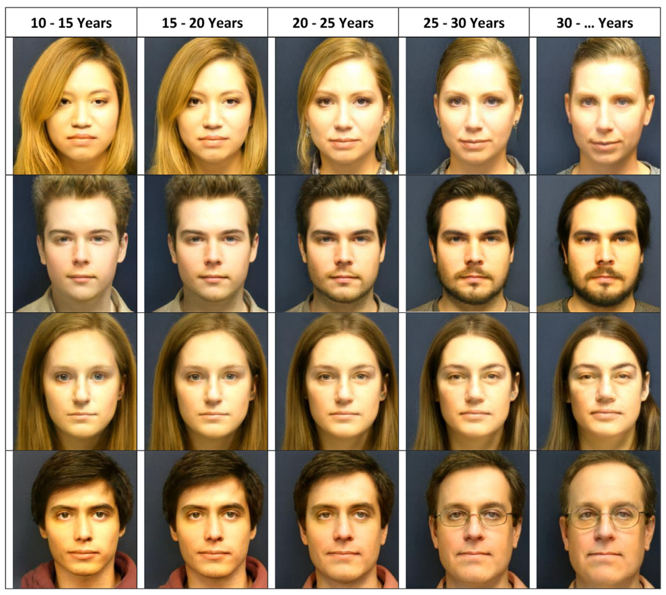
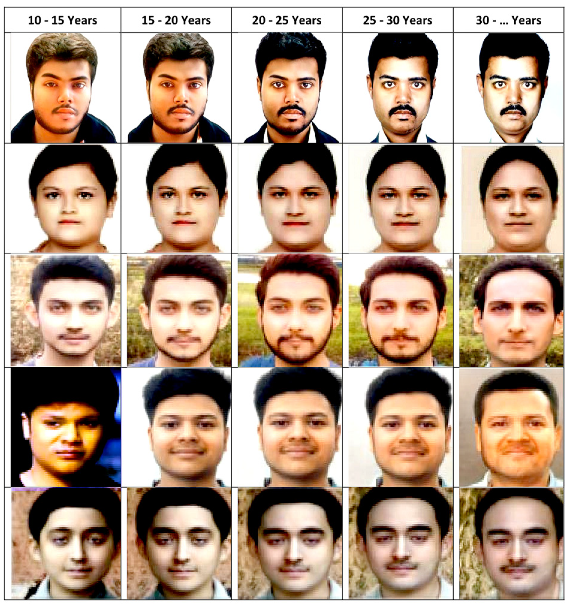
  • The proposed approach generates future faces that help to continue the investigation, using the Tufts [4] dataset.
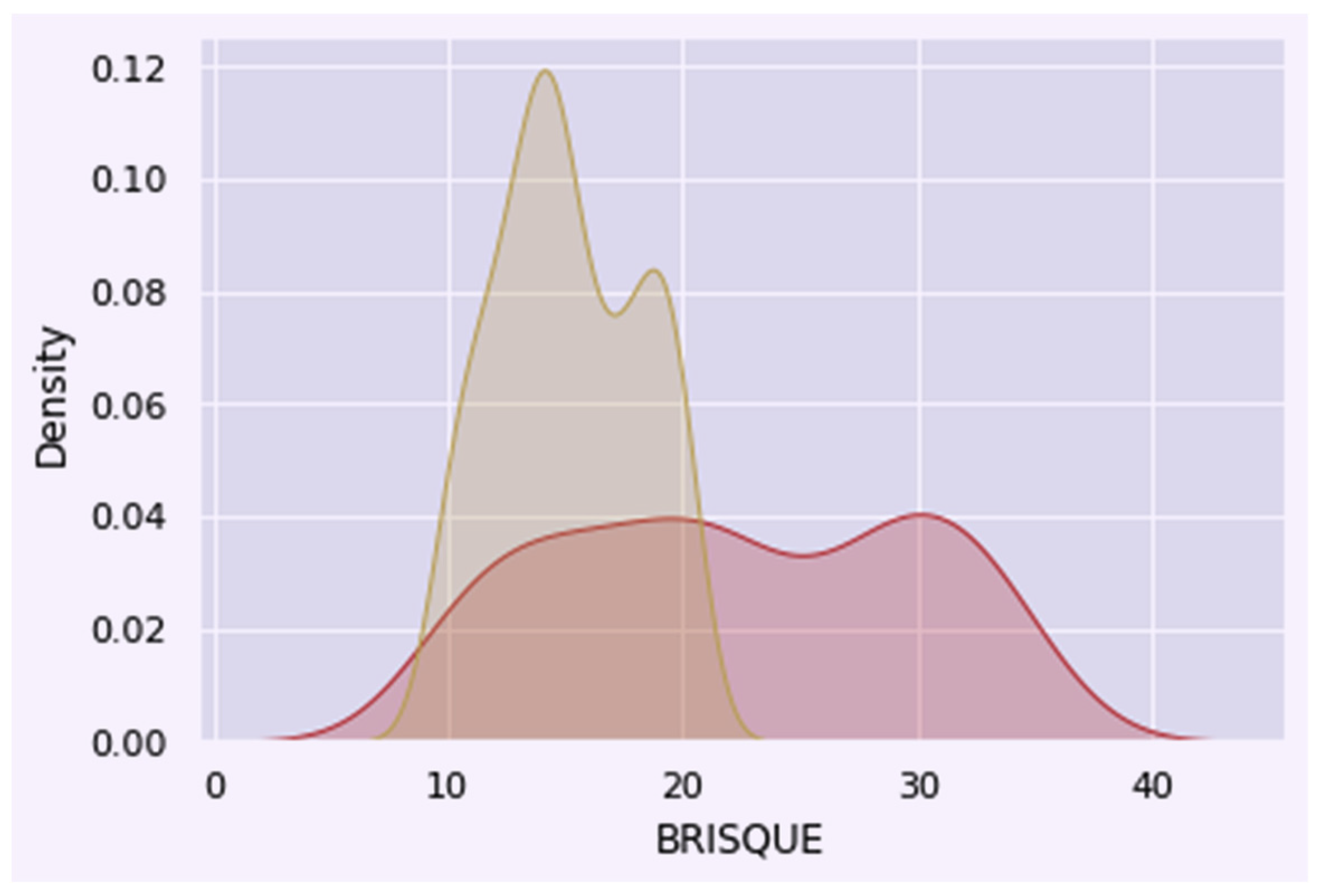
  • The BRISQUE quality metrics are analyzed to illustrate model-generated images’ visual quality using KINFACE I and KINFACE II datasets.
  • An extensive experiment was carried out to compare the original parent image with the model-generated children’s ideas of equal age using MSE, MSSSIM, ERGAS, SCC, RASE, SAM, and VIFP.
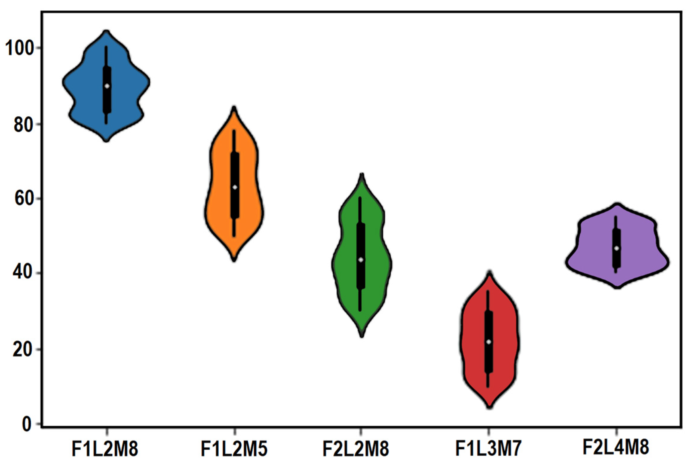
  • Various hyper parameters such as F1L2M8, F2L3M5, F2L2M8, F1L3M7, and F2L4M3 compare the proposed model-generated images.

4. Background Analysis

We use the convolution method as a kernel to extract features from images and modify the input as a matrix, referred to as a kernel which enhances the output. During this modification process, V as a convolution kernel with probability h, normally distributed, is measured as   Z θ ( e ) = V × e + θ [1]. Instead of manual extraction by Equation (1), CNN learn v extracts latent feature e by Z θ ( e ) . The following are a few important properties of the Cauchy distribution:
  • Multidimensional Cauchy distribution can be used to fill the latent space for any random variable u:
C ν ( u ) = 1 π 1 + u 2   u   Є  
Here, 1 π act as a density function.
  • In the absence of an appropriate moment generating function, the characteristic function is defined as follows:
  Φ u ( ν ) = E [ e ivU ]
where i = 1   and   v   is   a   real   number
| Φ u ( ν ) | = | E [ e ivU ] |   E [ | e ivU | ]   1
| e i v U | = 1   , where v is a real valued random variable.
  • The value of distribution Φ u ( ν ) greater than one may produce a negative impact on the GAN training process. It leads to the inappropriate formation of data points for generator-generated samples.
  • In order to train the proposed GAN model with latent space e , n independent random variables U 1 ,   U 2 ,   ,   U N   are   distributed with a fixed latent probability distribution as follows:
U 1 + U 2 + + U N ( ν ) = Φ   U 1 ( ν ) Φ   U 2 ( ν ) Φ   U 3 ( ν )   . Φ   Un ( ν )
  • The augmentation strategies in our proposed work are closely related to the approaches referred to as random masking [16]. This combines regularizing with augmentation of the existing data for better model performance: the projection of a random subset of dimension interpreted by cut-out augmentation. For a set of deterministic projections R 1 , R 2 ,   , R N , the condition is defined as R i 2 = R i   . Such projections include pixel permutation [17], scaling, and squeezing [18,19,20]. The discrete probabilities to choose identity operator O i are r 0 , r 1 ,     r n . For remaining discrete probabilities, it is RK. The mixed form of the projection is represented as follows:
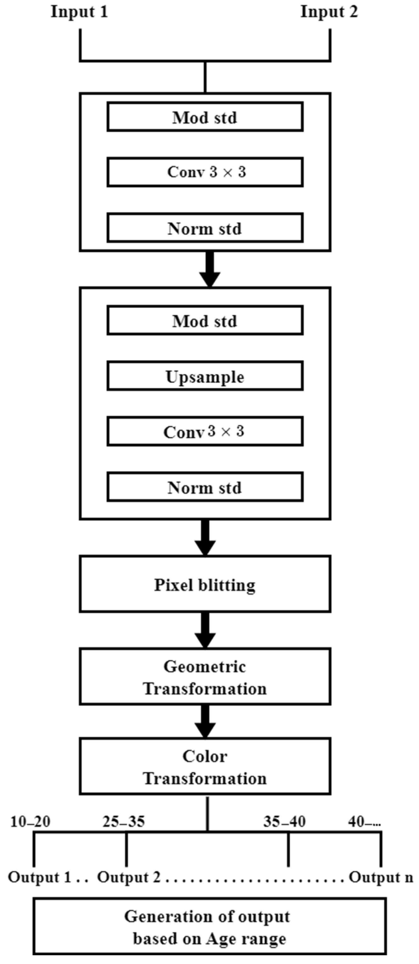
μ ρ = r 0 O i + i = 1 N   r i R i
For probability distribution z ≠ 0 and μ ρ z = 0 , the representation of this combination becomes the following:
r 0 z + i = 1 N   r i R i z = μ ρ z = 0 = i = 1 N   r i R i z       = r o z
Applying the theorem mentioned in Ambient GAN [21], probability for block pixel measurement, where n   Є   t i Є i if t > 1 , there exists a unique distribution t n r   and t m g for a given dataset, = Ω   ( | t | 2 i ( 1 t ) ϵ 2 2 i   log   ( | t | i δ ) ) where ϵ > 0   and   δ   Є   ( 0 , 1 )   Equation (5) becomes, i = 1 N   r i ( z , R i Z ) = r 0 Z , z .

5. Proposed Method

Overview of the FLM approach represented in Figure 1. The proposed method performs pixel blitting by duplicating pre-existing pixels. This operation does not blend with adjacent pixels. The adjustments aggregate into a 3 × 3 matrix V with input pixel ( a i , b ) placed as the output [ a 0 , b , 1 ] T = V [ a i , b i , 1 ] T x flip applied to each transformation with probability P by sampling i ~ μ { 0 , 1 } uniform distribution, then update V   by scale ( 1 2 i , 1 ) V . If rotation is applied to sample i ~ μ { 0 , 3 } ,   then   V is updated to rotate ( π 2 i ) V . Apply the integer translation to sample t a , t b ~ μ ( 0.125   , + 0.125 ) . During this translation, V is updated to translate ( round ( t a w ) , round ( t b h ) ) Matrix   V sample parameter s from a log normal distribution as s ~ N ( 0 , ( 0   2 , 1 n 2 ) 2 ) . Further general geometric transformation can be achieved by isotropic scaling of the sample   θ ~ μ ( π , + π ) and setting   Rotate ( θ ) V , then performing arbitrary rotation. Anisotropic scaling is performed along with fractional transformation with probability P by sample t a , t b ~ N ( 0 , ( 0.125 ) 2 )   and updating translate ( t a w , t b h ) V . Padding the image with reflection is done to avoid the unwanted effect of the image boundaries. The orthogonal low pass filter O ( z ) calculates the amount of padding by ( P 0 , P ni ) = CalcPad ( V , W , h , O ( P ) ) J = Pad ( J , P lo , P hi , reflect ) . Placing the origin at the image center is achieved by C = Translate ( 1 2 w 1 2 + P lo   , a   ,   1 2 h   ,   P lo   ,   b ) and V = C V C 1 . The method then up-samples J 1 = Upsample ( J , θ ( z 1 ) ) . Bilinear interpolation is applied to this higher resolution image. Down-sampling operation is applied to ( J , O ( z ) ) . Finally, color transformation is applied to gather the parameters of each separate transformation into 4 × 4 matrix. Sample θ ~ μ ( π , + π ) and setting R o t a t e ( θ ) V is conducted, followed by then performing arbitrary rotation. Anisotropic scaling is performed with fractional transformation with probability P by sample t a , t b ~ N ( 0 , ( 0.125 ) 2 ) and updating translation ( t a w , t b h ) V .

5.1. Data Augmentation

Machine learning systems of image augmentation improve instance segmentation-based image policies. Applying augmentation policies in models during training improves performances and accuracy for learned data. The augmentation approaches improve model accuracy and robustness by reducing overfitting. Few approaches like jittering helps to generalize different lighting conditions of contrast and saturation. Concerning the neural architecture search (NAS), the selection of an improper optimization procedure leads to increased computational complexity and computation cost. The optimal magnitude influences the training procedure in population-based augmentation (PBA 1). In our proposed method, Rand Augment [11] reduces computational expense caused by the search phase implementing several search policies [1,10,22]. The proposed system uses uniform probability to choose transformation to maintain image diversity.

5.2. Pixel Blitting

In order to detect pixel level errors, the discriminator implements rotation for geometric transformation. The given image accumulates into a matrix M of pixel values. The probability P is applied with x flip upon matrix M by M |   = x ( M ) . The M | is then periodically updated by sampling via discrete U {.} or continuous U (.) uniform distribution.   90 ° rotation is applied with sample 𝒾   ~   U { 0 , 3 } . Finally, the M R | updated ( M | M R | ) to T ( M R | ) by applying the translation matrix.
T   = [ 1 0 0 0 1 0 0.125 0.125 1 ]

5.3. Geometric Transformation

The proposed approach starts sampling t normally distributed with mean 0 and variance 1. The parameter S is evaluated via base 2 exponent of   0.2 *   t . Sample S is log normally distributed with μ = 0 , σ 2 = ( 0.2 · ln · 2 ) 2 . The previous probability is updated to   P | 1 1 P . The proposed approach performs uniform distribution upon sample θ with parameter π and   π . The previous pixel matrix is again updated as follows:
T | ( M R | ) [ cos θ sin θ 0 sin θ cos θ 0 0 0 1 ] T ( M R | )
After anisotropic scaling again with probability P , the parameters of the translation matrix show a normal distribution with mean 0 and variance ( 0.125 ) 2 [ T | | ( M R | ) ] . The geometric transformation is executed by setting up padding based on reflection. The amount of padding is evaluated based on   T (   M   R ) bilinear interpolation that is carried out through up-sampling and down-sampling of isotropic scaling value interpolation. The proposed approach uses sym6 to maintain the balance between model execution cost and sampling quality.

5.4. Color Transformation

The transformation starts by setting a homogeneous 3 d transformation brightness which is applied based on the probability where samples are normally distributed with μ = 0   and   σ = 0.2 . Uniform distribution is applied to achieve a Luma flip. We carried out Hue notation via a rotation matrix and ended the process with saturation through log-normal distribution.

6. Results

6.1. The proposed model accuracy evaluation with Similarity Index Evaluation Metrices

Image Quality Assessment (IQA) compares the amount of degradation with the perceived image. Inappropriate correlation leads to a reduction of image quality and was reflected as noise. Transmission, compression, enhancement, and acquisition are the features that play an essential role in the case of visual information analysis. Table 1 and Table 2 were performed on naturally existing persons. The model generated column contains images generated via the FLM approach compared with the original image. We chose children aged between 7 and 18 years for this experiment with their birth parents. The Image Quality Assessment quantifies with the mean square error (MSE) [21]. It evaluates the quality via the mean square deviation method.
MSE   = 1 IJ j = 0 I i = 1 J [ k ^ ( x , y ) k ( x , y ) ] 2
Here, MSE evaluation is conducted between two images, K ( m , n )   and K ^ ( m , n ) , to obtain the forecasting error root mean square error used to evaluate the absolute error.
RMSE   = M S E
PSNR (Peak Signal to Noise Ratio) [21] uses the logarithmic decibel scale to obtain a wide dynamic range. A ratio is obtained of possible signal power compared with distorting noise. The evaluation is expressed as follows:
PSNR   = 10 log 10 ( p 2 ) / MSE
where p represents the peak value. Important perception-based facts are evaluated with the help of the Structure Similarity Index (SSIM) [21]. The measurement is expressed as follows:
SSIM   = ˥ N ( m , n ) . K = 1 N F K ( m , n ) T K ( m , n   )
where the scale N represents the highest scale, F K ( m , n ) represents the contrast compression, and T K ( m , n ) represents the structure compression. ˥ N ( m , n ) is the compression based on luminance. They are evaluated by the following equations:
˥ N ( m , n ) = 2 μ m μ n + c 1 μ m 2 + μ n 2 + c 1
F K ( m , n ) = 2 σ m σ n + c 2 σ m 2 + σ n 2 + c 2
T K ( m , n ) = σ m n + c 3 σ m σ n + c 3
Here, μ m , μ n are the local mean, σ m , σ n =   standard   deviation   and σ m n = covariance for image.
The evaluation based on Table 1 and Table 2 observes that the MSE score ranges from 1 k to 5 k. Results with MSE score below 6 k expected to be perfect for similarity index. The proposed approach obtains RMSE between 30 and 80; lower RMSE reflects better accuracy. The PSNR score in Table 1 is better in comparison to Table 2. SSIM index also scores better for the proposed method.

6.2. FLM Model Performance Evaluation-Based Multiscale Extension, Spectral Property, and Visual Information

Multiscale extension SSIM (MSSSIM) [23] is the extension of SSIM that focus on low-pass sub-sampling and filtering through variance and cross-correlation. The FLM approach was tested on MSSSIM with a score of less than 0.5, representing edge similarities in Table 3 images across the image scale. In some situations, for images with different spatial resolutions, the comparison is performed using Error Relative Global Dim Synthesis (ERGAS) [24]. ERGAS-based comparative approaches applied in Table 3 obtained results below 30 k. A close score of less than 20 k represents the similarity based on correlation and normalization. A Relative Average Square Error (RASE) [25] score ranging average to 3 k means good similarity among all the generated images. The Spectral Angle Mapper (SAM) evaluates the spectral angle formed between two image spectrums [26]. SAM treats image bands as vectors in spectral space. The angle with the lower value represents a closer match between the two image spectrums. In the table, our proposed approach secured a meager SAM value reflecting our model’s efficiency. Visual Information Fidelity (VIFp) [27] achieves scores close to zero, representing close similarity among the model-generated and original images.

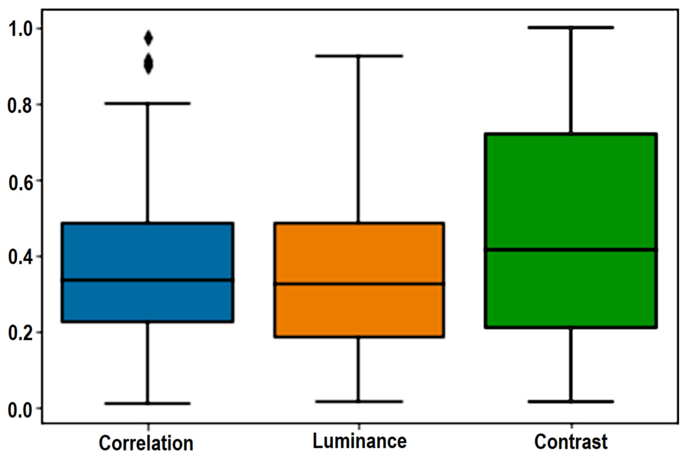
6.3. Experiment carried out for the Level of Distortion Using Universal Quality Index

To observe the level of distortion in our generated output of the proposed approach, the Universal Image Quality Index (UIQI) [28] was evaluated on 100 selected images of the KinfaceW dataset. UIQI metric is a full reference image quality assessment technique to evaluate quality of an image by comparison. UIQI takes into account both enhance-ment and restoration for assessing the quality of image. The scores measured locally combined with the local region plotted in Figure 2. From Figure 2, it is observed that the loss of correlation and luminance distortion are in the proper balance within 0.2 to 0.5. Contrast distortions are also close but slightly more significant compared to other factors. For future work, this factor helps to set the hyper parameter to maintain all three aspects in equal measure, with the lower value representing a closer match between the two image spectrums. In the table, our proposed approach secured a meager SAM value reflecting our model’s efficiency. Visual Information Fidelity (VIFp) [27] achieves scores close to zero, representing close similarity among the model-generated and original images.

6.4. Experiment for the Level of Distortion Using Universal Quality Index

FLM-generated images are very natural and difficult to distinguish as a machine generated output. To check the quality of the generated images, Blind/Reference less Image spatial Quality Evaluator (BRISQUE) [29] was applied on the results of the kinfaceW [30] dataset.
BRISQUE [29] first measures the distortion amount and prepares to extract natural scene statistics. Next, the pairwise neighborhood relationship using pixel intensities as a vector is established by subtracting the contrast normalization. In Figure 3, the red section represents the result evaluated on Kinface II, and the yellow bar represents Kinface I, two separate parts of the same dataset. Figure 3 shows that the proposed work achieves an excellent BRISQUE score for the Kinface I value ranging from 10 to 20. In Kinface II, the result varies depending on multiple images. Take this as the average.

6.5. Experiment for Hyperparameter Selection

The proposed model tests 200 images of the KinfaceW [30] and Tufts [4] datasets. The dataset [30] contains unconstrained face images specially designed for kinship verification. The data are organized as a pair to determine the kin relationship between father, mother, daughter, and son.
The four biological relationships distribute within 134, 156, 127, and 116 pairs. Moreover, another part of the dataset [30] consists of 250 pairs of images. The KinfaceW [30] images are applied to the proposed approach to evaluate the future appearance of the children. The human observer assesses the generator-generated images. The KinfaceW dataset designed to automatically determine kin or non-kin pairs through preserving facial expression based on genealogy records. This dataset provides valuable resource for biometric authentication, forensic investigations and genealogy research. The violin plot in Figure 4 represents the various hyperparameter evaluations based on the proposed method. Feature map one, learning rate two, and mapping net depth eight are F1L2M8. Based on this hyperparameter, the investigating officers generate the future appearance of the lost children based on the input such as in Figure 5, Figure 6 and Figure 7.

6.6. Comparison Carried Out with Other Related Models

This section represents comparison between proposed work with other related state of the art models. Table 4 illustrates conceptual comparison along with limitations. Table 5, Table 6, Table 7 and Table 8 contains detailed hyperparametric and architectural implementation details of other similar approaches compared with our FLM approach of Table 9.
The architecture maintains style mixing by providing latent based inference evaluation. The order of magnitude amplifies features with style modulation. The learned affline transformation combines normalization with phase modulation during feature convolution. The architecture scales the convolution weight such that w   c =   s k w , where w is the original weight and w   c represents the modulated weight. s k represents the scale corresponding to kth infant. Instant normalization updates output feature maps by eliminating the result of s k from statistics. The standard deviation of the output activation is updated.
σ i = i K     w c k i 2
The demodulation is similar to the re-parameterized weight tensor. Formulate regularizations, [ I ] m , n   ~   N ( O , T ) ( K S P χ 2 b ) 2 , where k s represents the Jacobian matrix, X are random images, K S P represents explicit computation of the Jacobian matrix latent space point S , and the scale of the gradient is represented as b   Є   . AMFIFV [13] and uses Darwin’s theory of natural evolution with (1+1)-ES algorithm [37] to prepare the initial population formulation on the face. Affline transformation acts as a mutation operator with scale and transformation parameters. The image deformation performed via warp generation requires feature mapping with source images. This approach leads to scattered data interpolation problems. The proposed approach uses augmentation with pixel blitting that does not require an inverse distance weighted interpolation method. AFR [14] uses Benford Features and a linear SVM classifier to perform training.
VAFM [33] is a software-based approach that uses the OpenCV landmark-based algorithm with WebMorph [41], an online tool and convolution layer for training [42,43,44]. FaceMorpher [33] is an open-source platform with a STASM [45] landmark detector. In Table 8, VAFM [33] is restricted to the FRLL dataset and is unable to obtain the expected result in another database such as FERET and FRGC [46]. The article also shows the calculations of MSE, RMSE, and PSNR [47,48]. Evaluation is performed on the parameters using 60 to 80 pixel cropping, an average of one scaling factor, and a minus three to three (degree) rotation angle. The AFR [14] approach in Table 9 lacks tampering detection. The AFR [14] also contains visual flaws while extracting the facial landmark.

7. Conclusions

The proposed approach obtains a BRISQE score within 10–30 by applying various flip and rotation mechanisms during pixel blitting. The score evaluated by comparing contrast, luminance and texture of the model generated pictorial statistics. Combining scaling and a few probabilistic transformations with StyleGan-ADA, the model obtains an SSIM score of 0.2 to 0.5 and MSSIM. For quality evaluation, the model brings a loss of correlation and luminance distortion within 0.2 to 0.5 during UQI [25] indexing. For future work, a few parameters need to change to balance the contrast distortion with loss of correlation and luminance distortion. To evaluate correlation and normalization, the proposed model scores 12 k to 23 k for ERGAS. The image spectrum was measured using SAM [26], score between, 0.2 to 0.5, reflecting its efficiency for generating output with reasonable accuracy. Such applications can also use for bioinformatics and other medical applications [49,50,51].
To carry out further research during pixel blitting, one can apply more color transformation strategies which improves the visual information fidelity (VIFP) score. During the experiment on hyperparameters, FLL2M5 scores quite near to the proposed FIL2M8.

Author Contributions

Conceptualization, methodology, and validation: B.B., B.D. and J.C.D.; formal analysis and investigation: B.B., S.K. and N.B.; resources and writing—review: B.B., B.D. and S.M.; writing—review and editing: S.M. and D.D. All authors have read and agreed to the published version of the manuscript.

Funding

This research received no external funding.

Data Availability Statement

Acknowledgments

The authors would like to thank all the lab members of our institutes for their valuable suggestions, which improved the quality of the article.

Conflicts of Interest

The authors declare no conflict of interest.

Abbreviations

V Convolution Kernel
Z θ ( e )     Feature extraction function
e Latent Feature
C ν Cauchy Distribution
u For any random variable
  Φ u ( ν )   Generating Function
U 1 ,   U 2 ,   ,   U N           Independent random variable distributed with fixed latent
R 1 , R 2 ,   , R N   Set of deterministic projection
O i Identity Operator
t n r   and t m g Unique Distribution
t a , t b   Transformation Variable
Θ Rotation Angle
( P 0 , P ni ) Variable for padding
U (.)Uniform Distribution
M Pixel value accumulated into matrix for image
T Translation Matrix

References

  1. Karras, T.; Aittala, M.; Hellsten, J.; Laine, S.; Lehtinen, J.; Aila, T. Training generative adversarial networks with limited data. Adv. Neural Inf. Process. Syst. 2020, 33, 12104–12114. [Google Scholar]
  2. Kennett, D. Using genetic genealogy databases in missing persons cases and to develop suspect leads in violent crimes. Forensic Sci. Int. 2019, 301, 107–117. [Google Scholar] [CrossRef] [PubMed]
  3. Tong, C.; Li, Y.; Jacob, A.P.; Bengio, Y.; Li, W. Mode regularized generative adversarial networks. arXiv 2016, arXiv:1612.02136. [Google Scholar]
  4. Karen, P.; Wan, Q.; Agaian, S.; Rajeev, S.; Kamath, S.; Rajendran, R.; Rao, S.; Rao, S.P.; Kaszowska, A.; Taylor, H.; et al. A comprehensive database for benchmarking imaging systems. IEEE Trans. Pattern Anal. Mach. Intell. 2018, 42, 509–520. [Google Scholar]
  5. Teterwak, P.; Sarna, A.; Krishnan, D.; Maschinot, A.; Belanger, D.; Liu, C.; Freeman, W.T. Boundless: Generative adversarial networks for image extension. In Proceedings of the IEEE/CVF International Conference on Computer Vision, San Francisco, CA, USA, 19 June 1985; pp. 10521–10530. [Google Scholar]
  6. Cai, Z.; Xiong, Z.; Xu, H.; Wang, P.; Li, W.; Pan, Y. Generative adversarial networks: A survey toward private and secure applications. ACM Comput. Surv. (CSUR) 2021, 54, 1–38. [Google Scholar] [CrossRef]
  7. Jabbar, A.; Li, X.; Omar, B. A survey on generative adversarial networks: Variants, applications, and training. ACM Comput. Surv. (CSUR) 2021, 54, 1–49. [Google Scholar] [CrossRef]
  8. Pascual, S.; Bonafonte, A.; Serra, J. SEGAN: Speech enhancement generative adversarial network. arXiv 2017, arXiv:1703.09452. [Google Scholar]
  9. Yufan, Z.; Chen, C.; Xu, J. Learning High-Dimensional Distributions with Latent Neural Fokker-Planck Kernels. arXiv 2021, arXiv:2105.04538. [Google Scholar]
  10. Goodfellow, I.; Pouget-Abadie, J.; Mirza, M.; Xu, B.; Warde-Farley, D.; Ozair, S.; Courville, A.; Bengio, Y. Generative adversarial networks. Commun. ACM 2020, 63, 139–144. [Google Scholar] [CrossRef]
  11. Zhang, H.; Venkatesh, S.; Ramachandra, R.; Raja, K.; Damer, N.; Busch, C. MIPGAN-Generating Strong and High Quality Morphing Attacks Using Identity Prior Driven GAN. IEEE Trans. Biom. Behav. Identity Sci. 2021, 3, 365–383. [Google Scholar] [CrossRef]
  12. Schaefer, S.; McPhail, T.; Warren, J. Image deformation using moving least squares. In ACM SIGGRAPH 2006 Papers; Association for Computing Machinery: New York, NY, USA, 2006; pp. 533–540. [Google Scholar]
  13. Bichsel, M. Automatic interpolation and recognition of face images by morphing. In Proceedings of the Second International Conference on Automatic Face and Gesture Recognition, Killington, Vermont, 14–16 October 1996; IEEE: New York, NY, USA, 1996. [Google Scholar]
  14. Makrushin, A.; Neubert, T.; Dittmann, J. Automatic generation and detection of visually faultless facial morphs. In Proceedings of the International Conference on Computer Vision Theory and Applications, Porto, Portugal, 27 February–1 March 2017; SciTePress: Setubal, Portugal, 2017. [Google Scholar]
  15. Tero, K.; Laine, S.; Aila, T. A style-based generator architecture for generative adversarial networks. In Proceedings of the IEEE/CVF Conference on Computer Vision and Pattern Recognition, Long Beach, CA, USA, 15–20 June 2019; pp. 4401–4410. [Google Scholar]
  16. DeVries, T.; Taylor, G.W. Improved regularization of convolutional neural networks with cutout. arXiv 2017, arXiv:1708.04552. [Google Scholar]
  17. Anwar, S.; Meghana, S. A pixel permutation based image encryption technique using chaotic map. Multimed. Tools Appl. 2019, 78, 27569–27590. [Google Scholar] [CrossRef]
  18. Atkins, C.B.; Bouman, C.A.; Allebach, J.P. Optimal image scaling using pixel classification. In Proceedings of the 2001 International Conference on Image Processing (Cat. No. 01CH37205), Thessaloniki, Greece, 7–10 October 2001; IEEE: New York, NY, USA, 2001. [Google Scholar]
  19. Jamitzky, F.; Stark, R.W.; Bunk, W.; Thalhammer, S.; Räth, C.; Aschenbrenner, T.; Morfill, G.E.; Heckl, W.M. Scaling-index method as an image processing tool in scanning-probe microscopy. Ultramicroscopy 2001, 86, 241–246. [Google Scholar] [CrossRef] [PubMed]
  20. Prashanth, H.S.; Shashidhara, H.L.; Murthy, K.B. Image scaling comparison using universal image quality index. In Proceedings of the 2009 International Conference on Advances in Computing, Control, and Telecommunication Technologies, Bangalore, India, 28–29 December 2009; IEEE: New York, NY, USA, 2009. [Google Scholar]
  21. Bora, A.; Price, E.; Dimakis, A.G. AmbientGAN: Generative Models from Lossy Measurements, Vancouver Convention Center, Vancouver, BC, Canada, 30 April–3 May 2018; ICLR, 2018. [Google Scholar]
  22. The CIFAR-10 Dataset. Available online: https://www.cs.toronto.edu/~kriz/cifar.html (accessed on 2 February 2023).
  23. Rouse, D.M.; Hemami, S.S. Understanding and simplifying the structural similarity metric. In Proceedings of the 15th International Conference on Image Processing, Vietri sul Mare, Italy, 12 October 2008; IEEE: New York, NY, USA, 2008; pp. 1188–1191. [Google Scholar]
  24. Renza, D.; Martinez, E.; Arquero, A. A new approach to change detection in multispectral images by means of ERGAS index. IEEE Geosci. Remote Sens. Lett. 2012, 10, 76–80. [Google Scholar]
  25. Willmott, C.J.; Matsuura, K. Advantages of the mean absolute error (MAE) over the root mean square error (RMSE) in assessing average model performance. Clim. Res. 2005, 30, 79–82. [Google Scholar]
  26. Yang, C.; Everitt, J.H.; Bradford, J.M. Yield estimation from hyperspectral imagery using spectral angle mapper (SAM). Trans. ASABE 2008, 51, 729–737. [Google Scholar] [CrossRef]
  27. Kuo, T.Y.; Su, P.C.; Tsai, C.M. Improved visual information fidelity based on sensitivity characteristics of digital images. J. Vis. Commun. Image Represent. 2016, 40, 76–84. [Google Scholar] [CrossRef]
  28. Wang, Z.; Bovik, A.C. A universal image quality index. IEEE Signal Process. Lett. 2002, 9, 81–84. [Google Scholar] [CrossRef]
  29. Mittal, A.; Moorthy, A.K.; Bovik, A.C. Blind/referenceless image spatial quality evaluator. In Proceedings of the Conference Record of the Forty Fifth Asilomar Conference on Signals, Systems and Computers (ASILOMAR), Pacific Grove, CA, USA, 6–9 November 2011; IEEE: New York, NY, USA, 2011; pp. 723–727. [Google Scholar]
  30. Lu, J.; Zhou, X.; Tan, Y.P.; Shang, Y.; Zhou, J. Neighborhood repulsed metric learning for kinship verification. IEEE Trans. Pattern Anal. Mach. Intell. 2014, 7, 331–345. [Google Scholar]
  31. Psychological Image Collection at Stirling (PICS). Available online: http://pics.psych.stir.ac.uk/2D_face_sets.htm (accessed on 12 January 2023).
  32. FEI Face Database. Available online: http://fei.edu.br/~cet/facedatabase.htm (accessed on 8 February 2023).
  33. Eklavya, S.; Korshunov, P.; Colbois, L.; Marcel, S. Vulnerability analysis of face morphing attacks from landmarks and generative adversarial networks. arXiv 2020, arXiv:2012.05344. [Google Scholar]
  34. Khan, M.; Chakraborty, S.; Astya, R.; Khepra, S. Face detection and recognition using OpenCV. In Proceedings of the 2019 International Conference on Computing, Communication, and Intelligent Systems (ICCCIS), Greater Noida, India, 18–19 October 2019; pp. 116–119. [Google Scholar]
  35. Phillips, P.J.; Wechsler, H.; Huang, J.; Rauss, P.J. The FERET database and evaluation procedure for face-recognition algorithms. Image Vis. Comput. 1998, 4, 295–306. [Google Scholar]
  36. Phillips, P.J.; Flynn, P.J.; Scruggs, T.; Bowyer, K.W.; Chang, J.; Hoffman, K.; Marques, J.; Min, J.; Worek, W. Overview of the face recognition grand challenge. In Proceedings of the 2005 IEEE Computer Society Conference on Computer Vision and Pattern Recognition (CVPR’05), San Diego, CA, USA, 20–25 June 2005; IEEE: New York, NY, USA, 2005; Volume 1, pp. 947–954. [Google Scholar]
  37. Kozyra, K.; Trzyniec, K.; Popardowski, E.; Stachurska, M. Application for Recognizing Sign Language Gestures Based on an Artificial Neural Network. Sensors 2022, 22, 9864. [Google Scholar] [CrossRef] [PubMed]
  38. Back, T.; Gunter, R.; Hans-Paul, S. Evolutionary Programming and Evolution Strategies: Similarities and Differences. In Proceedings of the Second Annual Conference on Evolutionary Programming, Evolutionary Programming Society, San Francisco, CA, USA, 10–12 July 1993; pp. 11–22. [Google Scholar]
  39. Salimans, T.; Goodfellow, I.; Zaremba, W.; Cheung, V.; Radford, A.; Chen, X. Improved techniques for training GANs. In Proceedings of the 30th Conference on Neural Information Processing System (NIPS), Bercelona, Spain, 5–10 December 2016. [Google Scholar]
  40. Federic, P.; Keith, W. Computer Facial Animation; AK Peters: Wellesley, MA, USA, 1996. [Google Scholar]
  41. Lecture Notes Series on Computing: Volume 4, Computing in Euclidean Geometry, 2nd ed.; World Scientific: Singapore, 1995; pp. 225–265. Available online: https://www.worldscientific.com/worldscibooks/10.1142/2463#t=aboutBook (accessed on 11 December 2022).
  42. Das, H.S.; Das, A.; Neog, A.; Mallik, S.; Bora, K.; Zhao, Z. Early detection of Parkinson’s disease using fusion of discrete wavelet transformation and histograms of oriented gradients. Mathematics 2022, 10, 4218. [Google Scholar] [CrossRef]
  43. Ghosh, S.; Banerjee, S.; Das, S.; Hazra, A.; Mallik, S.; Zhao, Z.; Mukherji, A. Evaluation and Optimization of Biomedical Image-Based Deep Convolutional Neural Network Model for COVID-19 Status Classification. Appl. Sci. 2022, 12, 10787. [Google Scholar] [CrossRef]
  44. Bhandari, M.; Neupane, A.; Mallik, S.; Gaur, L.; Qin, H. Auguring Fake Face Images Using Dual Input Convolution Neural Network. J. Imaging 2022, 9, 3. [Google Scholar] [CrossRef] [PubMed]
  45. Liu, C.; Chen, K.; Xu, Y. Study of face recognition technology based on STASM and its application in video retrieval. In Computational Intelligence, Networked Systems and Their Applications: International Conference of Life System Modeling and Simulation, LSMS 2014 and International Conference on Intelligent Computing for Sustainable Energy and Environment, ICSEE 2014, Shanghai, China, 20–23 September 2014, Proceedings, Part II; Springer: Berlin/Heidelberg, Germany, 2014; pp. 219–227. [Google Scholar]
  46. Milborrow, S.; Nicolls, F. Active Shape Models with SIFT Descriptors and MARS; VISAPP: Setubal, Portugal, 2014. [Google Scholar]
  47. Saladi, S.; Karuna, Y.; Koppu, S.; Reddy, G.R.; Mohan, S.; Mallik, S.; Qin, H. Segmentation and Analysis Emphasizing Neonatal MRI Brain Images Using Machine Learning Techniques. Mathematics 2023, 11, 285. [Google Scholar] [CrossRef]
  48. Bora, K.; Mahanta, L.B.; Borah, K.; Chyrmang, G.; Barua, B.; Mallik, S.; Zhao, Z. Machine Learning Based Approach for Automated Cervical Dysplasia Detection Using Multi-Resolution Transform Domain Features. Mathematics 2022, 10, 4126. [Google Scholar] [CrossRef]
  49. Levi, O.; Mallik, M..; Arava, Y.S. ThrRS-Mediated Translation Regulation of the RNA Polymerase III Subunit RPC10 Occurs through an Element with Similarity to Cognate tRNA ASL and Affects tRNA Levels. Genes 2023, 14, 462. [Google Scholar] [CrossRef]
  50. Mallik, S.; Seth, S.; Bhadra, T.; Zhao, Z. A Linear Regression and Deep Learning Approach for Detecting Reliable Genetic Alterations in Cancer Using DNA Methylation and Gene Expression Data. Genes 2020, 11, 931. [Google Scholar] [CrossRef]
  51. Mallik, S.; Mukhopadhyay, A.; Maulik, U. ANWAR: Rank-based weighted association rule mining from gene expression and methylation data. IEEE Trans. Nanobioscience 2014, 14, 59–66. [Google Scholar]
Figure 1. Overview of the proposed FLM method.
Mathematics 11 01345 g001
Figure 2. UQI evaluation score plot of kinfaceW dataset.
Mathematics 11 01345 g002
Figure 3. BRISQUE result on kinfaceW dataset generated result.
Mathematics 11 01345 g003
Figure 4. Human observer evaluation score on Multiple Hyperparameter.
Mathematics 11 01345 g004
Figure 5. Model trained on F1L2M8 tested on Tufts face dataset sample set 1.
Mathematics 11 01345 g005
Figure 6. Model trained on F1L2M8 tested on Tufts face dataset sample set 2.
Mathematics 11 01345 g006
Figure 7. Model trained on F1L2M8 tested on selected real existing persons.
Mathematics 11 01345 g007
Table 1. MSE, RMSE, PSNR, and SSIM evaluation on real existing persons using the proposed approach.
Model Generated
Image
Original ImageMSERMSEPSNRSSIM
Mathematics 11 01345 i001Mathematics 11 01345 i0023505.102440.042512.5616(0.3667, 0.5163)
Mathematics 11 01345 i003Mathematics 11 01345 i0043605.108430.042511.4312(0.4334, 0.5132)
Mathematics 11 01345 i005Mathematics 11 01345 i0061505.103448.031613.2114(0.4667, 0.4328)
Mathematics 11 01345 i007Mathematics 11 01345 i0081202.627341.856111.1255(0.4107, 0.4630)
Mathematics 11 01345 i009Mathematics 11 01345 i0101403.688342.575713.2367(0.5817, 0.5532)
Mathematics 11 01345 i011Mathematics 11 01345 i0121515.686141.573114.1244(0.3836, 0.4111)
Mathematics 11 01345 i013Mathematics 11 01345 i0146419.210080.119910.0559(0.2712, 0.3246)
Mathematics 11 01345 i015Mathematics 11 01345 i0161906.797243.666815.3277(0.4908, 0.5103)
Table 2. MSE, RMSE, PSNR, and SSIM evaluation on sample images.
Model Generated
Image
Original ImageMSERMSEPSNRSSIM
Mathematics 11 01345 i017Mathematics 11 01345 i0182235.054550.342312.8512(0.5127, 0.5687)
Mathematics 11 01345 i019Mathematics 11 01345 i0202347.464945.347014.2722(0.5032, 0.6289)
Mathematics 11 01345 i021Mathematics 11 01345 i0222213.891341.070412.6132(0.5381, 0.6013)
Mathematics 11 01345 i023Mathematics 11 01345 i0242532.128146.358711.5791(0.6212, 0.6864)
Mathematics 11 01345 i025Mathematics 11 01345 i0262730.074452.250113.7690(0.5308, 0.6178)
Mathematics 11 01345 i027Mathematics 11 01345 i0282402.991549.020314.3232(0.5122, 0.5651)
Mathematics 11 01345 i029Mathematics 11 01345 i0302156.575846.438914.7931(0.5032, 0.6289)
Mathematics 11 01345 i031Mathematics 11 01345 i0325314.247672.898810.8763(0.5459, 0.5977)
Table 3. MSSSIM, ERGAS, RASE, SAM, and VIFP evaluated on sample images.
Model Generated
Image
Original ImageMSSSIMERGASRASESAMVIFP
Mathematics 11 01345 i033Mathematics 11 01345 i034(0.5021 + 0j)16,381.10311573.82160.35770.0892
Mathematics 11 01345 i035Mathematics 11 01345 i036(0.3174 + 0j)16,522.58012503.25240.31520.0823
Mathematics 11 01345 i037Mathematics 11 01345 i038(0.3667 + 0j)19,423.1972807.75060.27280.0557
Mathematics 11 01345 i039Mathematics 11 01345 i040(0.3250 + 0j)19,535.80212632.07590.32080.1354
Mathematics 11 01345 i041Mathematics 11 01345 i042(0.3067 + 0j)10,832.98072005.23240.30540.0720
Mathematics 11 01345 i043Mathematics 11 01345 i044(0.3100 + 0j)18,026.68012557.69520.37260.0990
Mathematics 11 01345 i045Mathematics 11 01345 i046(0.2519 + 0j)29,463.85124270.37930.54290.0299
Mathematics 11 01345 i047Mathematics 11 01345 i048(0.5167 + 0j)12,382.30811770.85130.31760.0993
Mathematics 11 01345 i049Mathematics 11 01345 i050(0.2121 + 0j)18,222.72272551.41870.25210.0382
Mathematics 11 01345 i051Mathematics 11 01345 i052(0.2568 + 0j)11,582.31762351.72260.38610.0392
Mathematics 11 01345 i053Mathematics 11 01345 i054(0.2428 + 0j)19,252.74212151.46840.24240.0186
Mathematics 11 01345 i055Mathematics 11 01345 i056(0.2167 + 0j)11,583.21722551.74250.28630.0595
Mathematics 11 01345 i057Mathematics 11 01345 i058(0.4250 + 0j)19,637.90012831.07890.46090.1253
Mathematics 11 01345 i059Mathematics 11 01345 i060(0.4067 + 0j)20,832.98073005.23240.40540.0720
Mathematics 11 01345 i061Mathematics 11 01345 i062(0.5100 + 0j)18,026.68012557.69520.37260.0990
Mathematics 11 01345 i063Mathematics 11 01345 i064(0.3355 + 0j)23,438.19783370.89040.42370.0716
Table 4. Comparison of the proposed work with related models.
ModelProposed WorkLimitationDataset
Latent Neural Fokker [9]
–Planck kernels
It is a latent distribution-based approach with a plug and play implementation of GAN-based methods.Dwinghyper-parameter tuning KL divergence became more sensitive.CIFARIO [22]
MIPGAN [11]The shelf verification and face recognition system [12] for studying vulnerability to generate new data.Pre-selection of ethnicity, Mad performance detonated in empirical evaluation.FFHQ [15]
AIRF [13]This approach combines optimal morph field with Gaussian distribution to evaluate Bayes’ formation.The illustration is implemented, or the images are grayscale.MIT face
AFR [14]This method extracts facial landmark coordinates and averages them, splicing the visual flaws with inverse warping.The local analysis of skin texture produces color inconsistencies.ECVP [31], FET [32]
VAFM [33]It is a combined approach based on OpenCV [34] and Face Morpher [33].Lack of quality index factors.FERET [35], FRGC [36], FRLL [37].
Our ModelIt is based on StyleGan ADA with enhanced augmentation and scaling features.Further research needs to be carried out for output quality improvement.FFHQ [15],
kinfaceW [30]
Table 5. Comparison of the proposed model with MIPGAN [11].
Model Generated
Image
Original Image
MIPGAN [11]
Network ArchitectureArchitecture of StyleGan [15]
ApproachThe input latent code embedded into an intermediate latent space.
Convolutional Layer 3 × 3
Feature Maps
Weight DemodulationStyleGan [15]
Path Length RegularizationX
Lazy RegularizationX
GPU
Mixed ProcessorX
Learning Rate 5
OptimizerAMSGrad [38]
Table 6. Comparison with model [31] based on AMFIFV [15].
Model Generated
Image
Original Image
AMFIFV [13]
Network Architecture/ModelSPFM (Simple parameterized Face Model) [39]
ApproachFrontal view-based metamorphosis with automatic uniform illumination.
Convolutional Layer --
Feature MapsSPFM [39]
Weight DemodulationInverse Distance
Path Length Regularization
Lazy RegularizationX
Number of GPU--
Mixed ProcessorX
Learning Rate --
Table 7. Comparison with model [31] based on AFR [15].
Model Generated
Image
Original Image
AFR [16]
Network ArchitectureDelaunay triangulations [40]
ApproachForward and Backward Mapping performed to warp
Convolutional Layer --
Feature Maps[14]
Weight Demodulation[14]
Path Length RegularizationX
Lazy RegularizationX
Number of GPU--
Mixed ProcessorX
Learning Rate --
Table 8. Comparison of the proposed model with VAFM [33].
Model Generated
Image
Original Image
VAFM [33]
Network ArchitectureFaceMorph [33], Webmorph [41]
Approach
Convolutional Layer --
Feature Maps--
Weight DemodulationSTASM [42]
Path Length RegularizationX
Lazy RegularizationX
Number of GPU
Mixed ProcessorX
Learning Rate
Table 9. The Proposed Approach.
Model Generated
Image
Original Image
Network ArchitectureRevised architecture of AISG [1]
ApproachBroken into modulation based on feature map
Convolutional Layer 3 × 3
Feature Maps
Weight DemodulationAISG [1]
Path Length Regularization
Lazy RegularizationX
Number of GPU1
Mixed ProcessorX
Learning Rate 2
Mapping Net Depth8
Disclaimer/Publisher’s Note: The statements, opinions and data contained in all publications are solely those of the individual author(s) and contributor(s) and not of MDPI and/or the editor(s). MDPI and/or the editor(s) disclaim responsibility for any injury to people or property resulting from any ideas, methods, instructions or products referred to in the content.

