Prediction of Coal Dilatancy Point Using Acoustic Emission Characteristics: Insight Experimental and Artificial Intelligence Approaches

Abstract

This research offers a combination of experimental and artificial approaches to estimate the dilatancy point under different coal conditions and develop an early warning system. The effect of water content on dilatancy point was investigated under uniaxial loading in three distinct states of coal: dry, natural, and water-saturated. Results showed that the stiffness-stress curve of coal in different states was affected differently at various stages of the process. Crack closure stages and the propagation of unstable cracks were accelerated by water. However, the water slowed the elastic deformation and the propagation of stable cracks. The peak strength, dilatancy stress, elastic modulus, and peak stress of natural and water-saturated coal were less than those of dry. An index that determines the dilatancy point was derived from the absolute strain energy rate. It was discovered that the crack initiation point and dilatancy point decreased with the increase in acoustic emission (AE) count. AE counts were utilized in artificial neural networks, random forest, and k-nearest neighbor approaches for predicting the dilatancy point. A comparison of the evaluation index revealed that artificial neural networks prediction was superior to others. The findings of this study may be valuable for predicting early failures in rock engineering.

1. Introduction

Coal’s mechanical properties and failure behavior are difficult to predict due to the complex outer geological conditions (e.g., tectonic structure and water intrusion) [1]. There is a complex mechanical environment at such depths, which results in prominent nonlinear mechanical properties of coal as well as the surrounding rock mass. The coal is exposed to a high degree of stress, high gas concentrations, high temperatures, and a highly compressive environment [2,3]. It is common practice in coal seams to use water injection and hydraulic flushing to reduce coal and gas outbursts, rock outbursts, coal dust, and spontaneous combustion of coal seams [4,5,6]. These hydraulic measures change the initial structural state of a coal seam, which has a substantial impact on its mechanical behavior and geophysical properties [7,8]. As a result of mining disturbances, dilatation is a mechanical phenomenon that occurs. Consequently, coal dilatancy generates fluctuations in the primary variables of coal [9]. According to rock mechanics, a dilatancy point occurs before the failure of the rock during the loading process. There is a direct relationship between the amount of water in the coal and the physio-mechanical properties of the rock, as well as the coal’s dilatancy point [10,11,12,13,14]. These effects influence the rock dilatancy point, which occurs earlier than in dry conditions, eventually leading to early rock failure [10]. The dilatancy point is an important structural factor contributing to rock engineering structures’ stability. Various processes cause coal samples to become saturated and lose their mechanical properties. Similarly, once the coal is dried in the mine due to high temperatures, its mechanical properties are also altered. Therefore, determining the rock dilatancy point at various coal states is crucial for providing an early warning for successful engineering project monitoring.

As a method for measuring rock stability in laboratories and engineering projects, acoustic emission monitoring (AE) is a mature technology that has been extensively used to monitor and predict coal failure in the past [15,16,17,18,19,20,21,22]. Considering energy fluctuations (which include elastic energy and dissipation energy), rock failure can be seen as a result of energy fluctuations [23]. The term unstable rock refers to rocks that fail due to energy [24,25]. Elastic waves are produced when a rock ruptures under a load because of the strain energy released [26]. In addition to dissipating rock energy, this material preserves information about the formation of rock fractures, which is crucial to a thorough understanding of the dissipation process. A series of sequence parameters, including counts, energy, and frequency characteristics, along with their three-dimensional positioning, can be used to interpret AE signals for the purpose of predicting the deformation and fracture of rocks by considering their characteristics over time, such as counts, energy, and frequency [27]. Researchers demonstrated that coal with varying water content reduced the release of elastic energy during the loading process, thereby weakening the AE signal. Additionally, AE energy was studied using the accelerating energy release theory and the distribution density function [2,3]. Despite the availability of the studies mentioned above, it is rare to find an AE that can be used to predict rock dilatancy points for coal in three different states (natural, water-saturated, and dry). To adequately monitor rock stabilization and early failure precursors, AE characteristics in dilatancy processes need to be explored in more detail. In addition, the available literature does not support the application of artificial intelligence (AI) for predicting rock dilatation points and other mechanical characteristics based on AE data. Despite this, a wide variety of AI-based algorithms were effectively applied to other rock engineering issues [28,29,30,31,32,33,34,35,36]. The AE characterization and AI-based algorithms are, therefore, essential for predicting rock dilatancy points.

To provide an early warning system for successful engineering project monitoring, we examined the dilatancy point of coal in different states under loading in the presence of AE. The coal samples were prepared in various states and subjected to uniaxial compression in order to achieve the stated objective. Sensors were attached to the coal samples during loading in order to collect acoustic emission (AE) data. Subsequently, the mechanical properties of the coal samples and their AE characteristics were analyzed in order to predict the dilatancy point. To calculate a new dilatancy point index, absolute dissipation strain energy rates were experimentally measured. In addition, the AE counts were used as an input parameter for AI approaches for predicting dilatancy points in stress–strain curves. The primary goal of this research is to estimate the rock dilatancy point under different coal conditions in order to develop an early warning system for engineering projects.

2. Materials and Methods

2.1. Sampling

For this research, samples were collected from the working face of a coal mine in the Shanxi province of China. Samples were prepared per the international rock mechanics standard and then used in laboratory experiments. The samples were drilled, wrapped in bubble film, and then delivered to the laboratory. Cylindrical-shaped samples with a 50 mm diameter and 100 mm height are shown in Figure 1. A total of 9 samples were collected from a total of twenty samples based on their batch and average density and divided into three groups: D, N, and S, of which the D and S groups were immersed in deionized water. These groups represented dry, natural saturated, and saturated samples, respectively. The samples were soaked in water for 24 h to achieve full saturation. During the drying process, samples from the D group were placed in an oven at 60 degrees Celsius for 24 h. The test results are summarized in

Table 1. The physio-mechanical parameters of saturated, dried, and natural coal samples.

Sample Number	State	Peak Stress (MPa)	Elastic Modulus (GPa)	Crack Initiation Stress (MPa)	Peak Strain 10−2	Dilatancy Stress (MPa)
D-1	Dry	16.1	1.280	5.2447	0.02257	14.7
D-2	Dry	16.3	1.259	5.194	0.01993	13.5
D-3	Dry	17.86	1.330	5.34	0.0264	15.0
N-1	Natural	10.73	0.946	4.3	0.0198	8.85
N-2	Natural	10.35	0.882	4.21	0.0138	8.55
N-3	Natural	9.70	0.841	3.9	0.0098	7.95
S-1	Saturated	5.92	0.721	2.599	0.01269	4.9
S-2	Saturated	5.5	0.683	2.556	0.01132	4.3
S-3	Saturated	6.7	0.755	2.88	0.01352	5.0

.

2.2. Experimental Scheme

The experimental scheme, illustrated in Figure 2, involves two main parts (1) a loading and sensing and (2) a data collection system.

The detail of the experimental scheme was as follows:

Figure 2. Experimental setup of the research.

Figure 2. Experimental setup of the research.

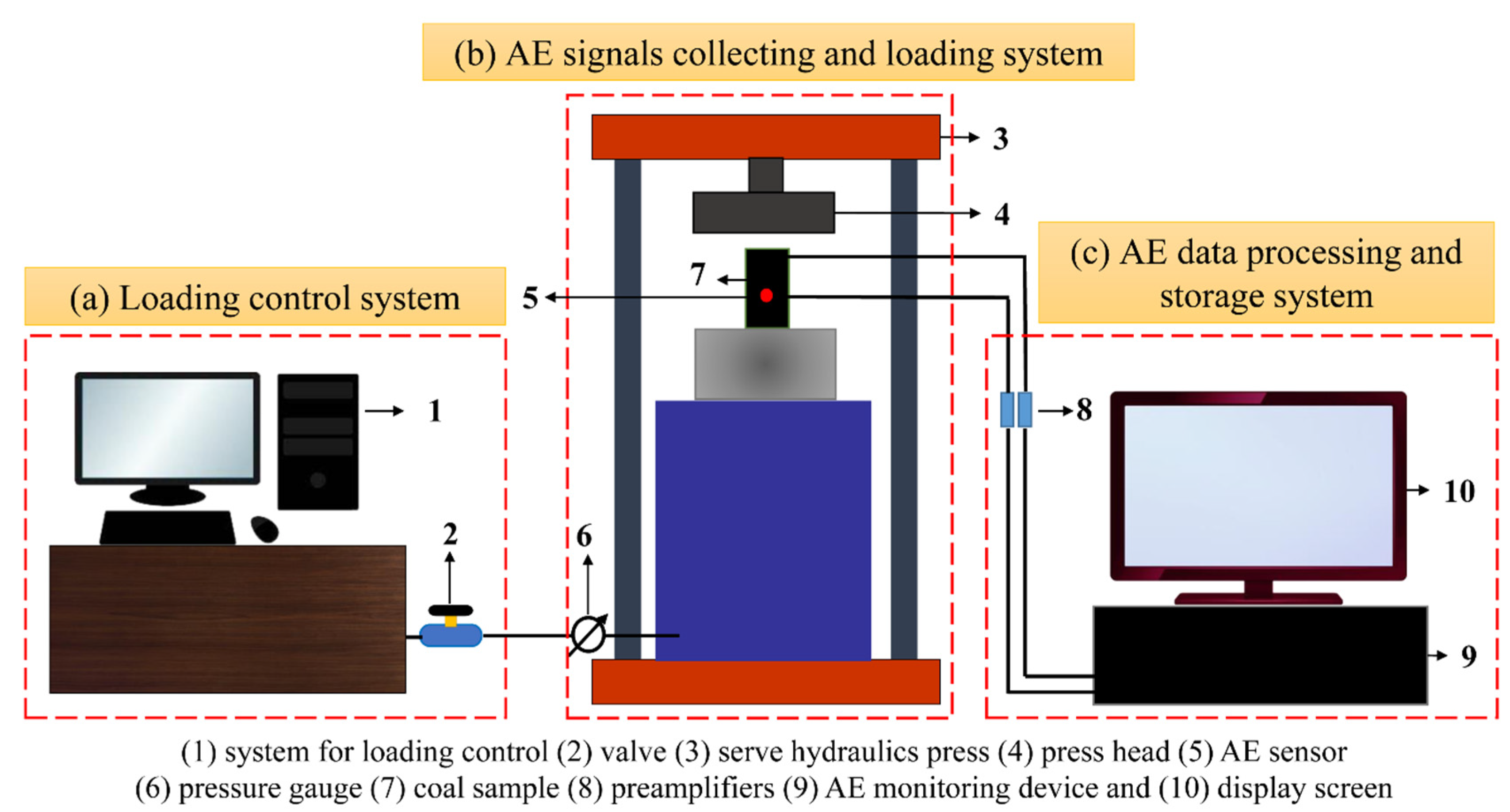
2.2.1. Loading System

The loading system is illustrated in Figure 3. This system comprised several uniaxial compression tests with (1) uniform loading, (2) cyclic loading, and (3) dynamic state. A 3000 kN pressure testing equipment (Y4306) was used for the loading system [37]. The system included a press host, a loading control system, a computer, and a power-test V33 control composition. During the experiment, the pressure head of the press produced pressure and displacement, which were transmitted with analog electrical signals to the loading control system via the pressure sensor and extensometer. Digital signals from the control system were transmitted to the computer, where the data signals were collected and stored by the software. The power-test V33 software drove the press via the control box to complete the loading operation in accordance with the manual instruction. Force and displacement data were sampled at up to a rate of 100 Hz. The experimental curves were recorded and displayed in real-time based on load time, deformation time, force deformation, and force displacement.

2.2.2. Data Collection System

The AE System (PCI-2), shown in Figure 4, was used to record the data. This system includes a digital-to-analog converter module with an A/D conversion rate of 18 bits, eight digital input/output channels, and two real-time data acquisition channels. Before the conversion module obtained the signal, the preamplifier amplified it. The amplifier provided three output levels: 20 dB, 40 dB, and 60 dB. AE sensors were equipped with a 20 dB electronic preamplifier that could respond to frequencies between 50 and 400 kHz.

3. Intelligent Model

3.1. Artificial Neural Network (ANN) Model

In geotechnical engineering, ANNs are considered intelligent tools for solving complex engineering problems [38,39]. The network consists of the input layer, the hidden layer, and the output layer. The number of neurons in each layer varies according to the particular application. The neurons of each layer are connected to those of the next layer, and each connection carries a certain amount of weight [40]. ANN model employs a number of algorithms, with backpropagation (BP) being the most efficient due to its simple training function. To train the BP algorithm, a group of examples was used to link and connect nodes and identify the parametric function (weight inadequate). By repeatedly reducing the mean square error (MSE), it is possible to minimize the discrepancy between actual and anticipated results. In addition, training facilitates the determination of the weights for each iteration. The BP method is often used when training various types of networks. An earlier study demonstrated that the BP method assumes a random value and takes this into account. As a result, the ANN operation uses this random value to compute the result. To reduce the margin of error, the weight is adjusted multiple times until the minimal result is achieved [10]. The model needs to be trained, and the literature contains recommendations on how to accomplish this [41].

3.2. Random Forest Regression (RFR)

RFR is used to facilitate the prediction of the stability of hanging walls by describing nonlinear interactions between inputs and outputs without making any statistical assumptions about the data. Thus, the procedure could be pinpointed. It is quite common for geotechnical engineers to use the RFR approach [42,43]. Zhou, Li [44] used it for the stability of rock pillars, Zhang, Wu [45] and Lagomarsino, Tofani [46] for landslide susceptibility assessment, Kohestani, Hassanlourad [47] for soil liquefaction potential, and Zhou, Shi [48] for ground settlement prediction. However, RFR has rarely been scientifically evaluated in relation to predicting the stability of hanging walls.

RFR makes predictions based on bagging the data, which serves as the foundation of this technique. Decorrelated decision trees (DTs) are formed by joining samples collected via the bagging method with samples collected using other methods. The results of averaging all DTs are used to improve the modeling quality without resorting to overfitting. Figure 5 illustrates the general architecture of RF. This figure represents the results of the individual DT as indicated by numbers k1, k2, etc., up to and including kn.

3.3. k-Nearest Neighbor (KNN)

KNN’s power and simplicity make it ideal for many applications [49]. In classification and regression, ANNs and RFs are similar techniques. This approach has advantages such as its easy comprehension and implementation. A nonlinear decision boundary can be learned if it is used for classification and regression, as well as an extremely flexible choice limit by adjusting the value of K and is capable of both. There is no dedicated training step in the KNN architecture. Due to the fact that there is only one hyperparameter, denoted by the letter K, it is quite simple to adjust the other hyperparameters.

Based on the calibration dataset, KNN locates a group of “k” samples close to unknown samples (for example, by applying distance functions). The sample groups may be compared by looking for similarities. As part of the KNN, the average of response variables is calculated and compared with the averages of the “k” samples to identify the class of unknown samples. Therefore, KNN performance depends heavily on k’s value [49]. Using Equations (1) to (3), the distance between neighboring points was calculated to analyze the regression issue:

$$\mathrm{F}(\mathrm{e})=\sqrt{{\displaystyle \sum _{\mathrm{i}=0}^{\mathrm{f}}({\mathrm{x}}_{\mathrm{i}}-{\mathrm{y}}_{\mathrm{i}}}}{)}^2$$

(1)

$$\mathrm{F}(\mathrm{m}\mathrm{a})={\displaystyle \sum _{\mathrm{i}=0}^{\mathrm{f}}\left|{\mathrm{x}}_{\mathrm{i}}-{\mathrm{y}}_{\mathrm{i}}\right|}$$

(2)

$$\mathrm{F}(\mathrm{m}\mathrm{a})={\left({{\displaystyle \sum _{\mathrm{i}=0}^{\mathrm{f}}\left(\left|{\mathrm{x}}_{\mathrm{i}}-{\mathrm{y}}_{\mathrm{i}}\right|\right)}}^{\mathrm{q}}\right)}^{\frac{1}{\mathrm{q}}}$$

(3)

This function has four components: F(e) = Euclidean function, F(ma), Manhattan function, F(mi) = Minkowski function, and xi, yi, and q.

4. Mechanical Characterization

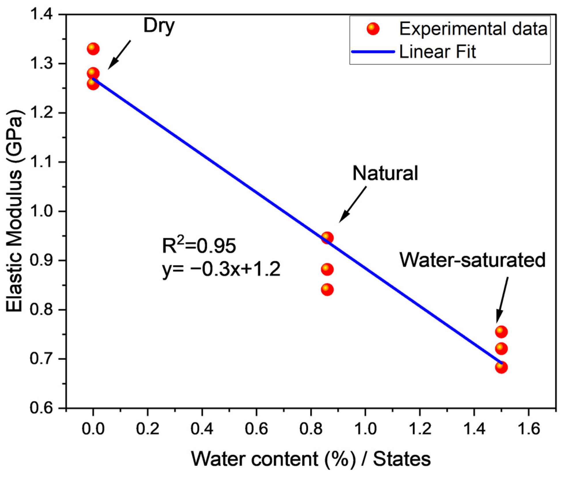
4.1. Elastic Modulus

Rock deformation is primarily caused by its intact elastic modulus (E), which corresponds to the stress–strain curve slope. A tangent modulus, a secant modulus, and an average modulus are the three methods for calculating it. The E was calculated from the stress–strain curve through the average modulus, using Equation (4) and assuming that σ = f(ε).

$$E=\frac{f({\epsilon }_2)-f({\epsilon }_1)}{({\epsilon }_2)-({\epsilon }_1)}$$

(4)

where f (ε₁) denotes the reference stress at the start of the elastic phase and f (ε₂) denotes the value of stress, whereas ε₁ and ε₂ represent the initial and final stain, respectively.

4.2. Stresses Associated with Dilatancy and Crack Initiation

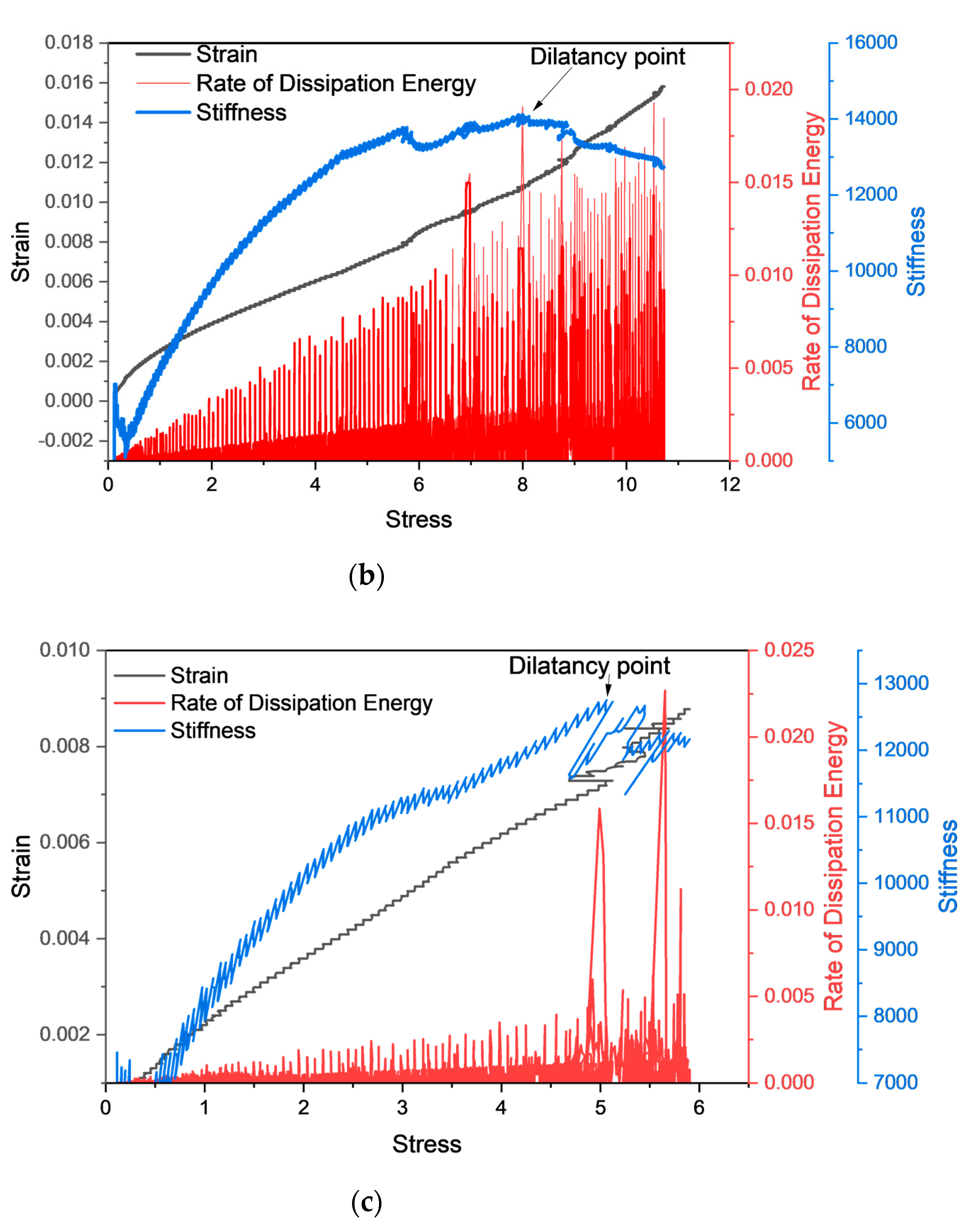
The crack closure, crack initiation, and dilatancy stresses were calculated from the stress–strain and stiffness–stress curves for the three batches of coal [50,51]. The test results are shown in Figure 6a–c, which illustrates the stiffness–stress and strain–stress curves under uniaxial loading. A point known as the crack closure (point A) was reached during the loading phase when both curves tended to converge. This curve climbed with loading until it reached the point of crack initiation (point B), where it reached its maximum curvature. Elastic deformation occurred at stage AB. In the stiffness curve, the slope rose progressively until point C, also known as the dilatancy point, which corresponded to the dilatancy stress. The fracture propagated continuously in segment BC. The curve gradually reached the maximum stress point D as loading increased, with the segment CD representing the propagation of unstable fractures. As a result, the rock sample produced audible sounds. The fractures rapidly widen, spread, and join together to form macro fracture surfaces, but the rock sample remains relatively undisturbed.

4.3. Strain Energy

The rock encounters dissipative and elastic strain energy during loading. The total strain can be calculated using the first law of thermodynamics, assuming that the rock does not lose heat during the loading process.

$$E=E_e+E_d$$

(5)

E denotes total strain energy, E_e represents elastic energy, and E_d refers to dissipated energy. The total strain energy was generally estimated from the area under the stress–strain curve. With loading, E_d is emitted during crack development and transmission while E_e is stored in the rock [10].

Calculations based on Equations (6)–(10) are possible for strain, dissipation strain, elastic strain, and the absolute rate of dissipation strain energy.

$$E={\displaystyle {\int }_0^{{\epsilon }_1}\partial \sigma {\epsilon }_1}$$

(6)

$$E_e=\frac{{\sigma }^2}{2E}$$

(7)

$$E_d=E-E_e$$

(8)

$$\Delta E_d=\frac{E_{d2}-E_{d1}}{t_2-t_1}$$

(9)

$$\left|\Delta E_d\right|=\left|\frac{E_{d2}-E_{d1}}{t_2-t_1}\right|$$

(10)

In the aforementioned equations, σ symbolizes axial stress, ε₁ denotes strain, E_d2 represents dissipation strain energy at the end position at time t₂, and E_d1 denotes dissipation strain energy at the beginning location at time t₁. The │ΔE_d│is the absolute rate of dissipated energy.

4.4. Water Content and Their Response to the Stress–Strain Curve

The water and coal interaction occur in a rich aquifer in the in situ environment due to any excavation operation during mining [52,53,54]. This interaction substantially impacts rock damage, reducing the mechanical characteristics of coals masses. The impact may cause a reduction in internal friction and bonding strength within the sample. This negative effect of water on the strength reveals that a lower dissipation strain energy would be required for the sample fracturing and micro-crack propagation [39]. The curves, stress–stiffness, strain, and stress were divided in different stages; crack closure stage (CCS), elastic deformation stage (EDS), stable propagation stage (SPS), and unstable propagation stage (USPS) [55]. The comparison of natural coal, dry coal, and saturated coal samples showed that the coal in different states exhibited different characteristics. In addition to decreasing the slopes of the curves, water also minimized the closure and propagation stages of cracks. In contrast, these water contents had the opposite effect on the EDS and USPS. Additionally, the disparity between CC and USPS in terms of stress and strain increased. As seen in Figure 6a, such variations declined in EDS and SCPS (c). Water content increased in the CCS and USCP stages, while the EDS and SCPS stages decreased. Table 1 illustrates the mechanical parameters of the stress–strain curve at various water contents.

Figure 7, Figure 8, Figure 9 and Figure 10 show the relationship between elastic modulus, peak stress, crack initiation stress, and dilatancy stress as a function of water content. Figure 7 depicts a negative linear correlation between elastic modulus and water content. It is concluded from Figure 7 that the elastic modulus declined with the increase in water content, as revealed in Table 1. In the case of peak stress and water content relation, a linear negative relation is shown in Figure 8. From Table 1, the peak stress of the dry sample was less than the natural sample but greater than the saturated sample. It can be observed in Figure 9 that the crack initiation of natural coal was 4.3 MPa, less than the dry sample’s initial crack stress of 5.2 MPa, but greater than the saturated coal sample, which was 2.80 MPa. The dilatancy point of the dry sample was approximately double that of natural coal while three times greater than saturated coal, as itemized in Table 1 and indicated in Figure 10. The water plays as a lubricating agent, resulting increase in the reduction in the rate of stress increase. Water reduces stress and increases the effect of weakening through its lubricating properties [39]. The rock encounters dissipative and elastic strain energy during loading. Assuming that the rock does not lose heat during the loading, the total strain can be calculated using the first law of thermodynamics.

As shown in Figure 11, stiffness, stress, and level of absolute dissipation energy in the three samples were determined. The results indicated that the absolute strain energy at the dilatancy point increased suddenly. This increase was due to the increase in volume at the point of dilatancy, which released a large amount of dissipation energy. The water content reduced the peak stress, resulting in an early dilatancy point in the D group, compared to the samples of the remaining two groups (N and S groups). In addition, even when the dried samples were compared with natural samples, the peak stress decreased when the water was removed by drying the sample. The two curves showed a drop at the dilatancy point, resulting in an absolute dissipation strain energy rise. In the early stages, this behavior was not identical to these curves. In spite of this, the significance of absolute dissipation strain energy, as described above, suggests a connection between the two curves. In Figure 11, the rise in absolute dissipation strain energy at a later stage caused a significant decrease in the corresponding strain–stress and stiffness–stress curves. It should be noted that stress levels associated with the initial abrupt change in absolute strain energy are analogous to those associated with other failure precursors used as early warning systems. The AE precursor occurs at around 79 percent of peak stress, as per the study by Wu, Liu [56]. Zhang, Li [57] observed the failure precursor of coal under uniaxial loading at approximately 90% of its peak stress. Wu, Gao [58] observed a failure precursor of brittle rock at approximately 80% of peak stress under uniaxial loading. Coal failure precursors amount to about 85 percent of the peak stress [57]. In summation, under a variety of conditions, a rapid change in stiffness–stress and absolute dissipation strain energy can serve as an early warning sign for coal failure.

4.5. Strain Energy Rate

Water plays a vital role in strain energy, showing a negative linear correlation with both total and elastic strain energy, while dissipation strain energy has an exponential correlation [59]. Under different water content conditions, strain energy for a dilatancy point was evaluated. At the dilatancy point, ΔE_d and amplitude rapidly grew and decreased with water content. However, dry sample amplitude decreased when correlated with the natural sample. This decrease was due to the dissipation energy which decreased with water content, as shown in Figure 12. Furthermore, it was observed that almost in all samples, rate of change in dissipation energy (ΔE_d) from the start of loading to peak stress was lower than ΔE_d at the point of dilatancy. This dissipation rate of strain energy evidently showed the dilatancy during the loading process under various water conditions. The average value of the absolute dissipation strain energy in the loading negatively correlates with water. This reveals an increase in the rock’s internal damage in the presence of water, ultimately lowering dissipation strain energy. In conclusion, the dissipation strain energy directly relates to the sample strength [60,61].

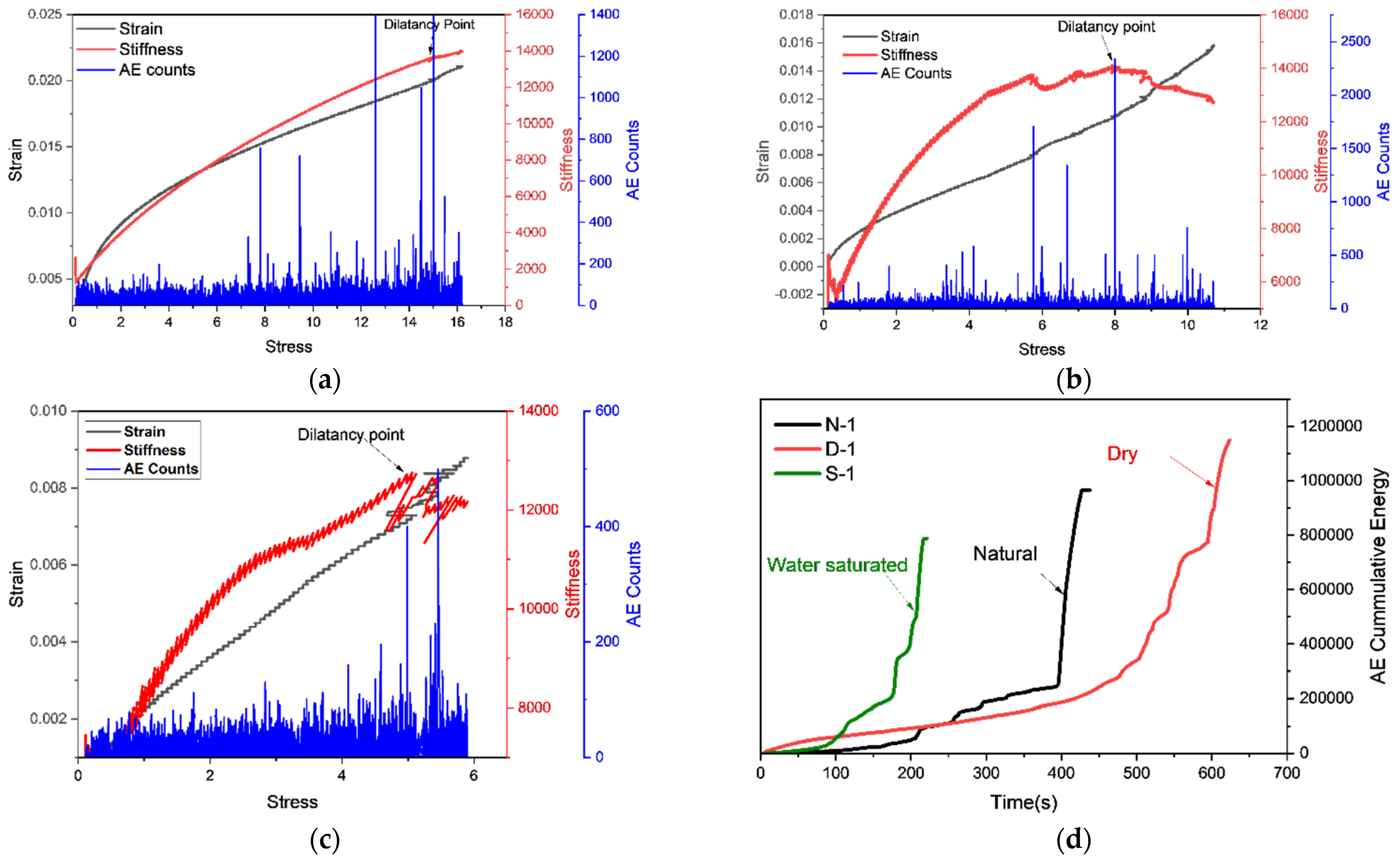
5. AE Counts Characteristics and Counts under Stress–Strain Curve Stages

A rapid elastic wave signal, known as AE, results from the sudden strain energy discharge in rock and other materials [2,62]. The energy produced by rocks can be reflected in AE signals. Water damages rock irreversibly, and as a result, it impacts the shape and intensity of the energy emitted from coal in the form of AE. It also exhibits the crack propagation criterion in failures [2,63]. To show the AE effects on the fracture damage in coal, the stress–strain AE counts along with stiffness are plotted in Figure 13. The figure reveals that AE counts varied depending on the amount of water in the crack and the stage of the crack. Under the stress–strain curve, the AE counts corresponded well with the crack generation. It can be concluded that stress and AE counts have an inverse relation. The rate of AE counts is defined at different stages of the stress–strain curve, including the CC, DS, SCP, and USCP stages. In natural conditions, their values are 100, 246, 155, and 1706, respectively. These values were 128, 330, 345, and 1049 in dry conditions and 68, 92, 101, and 499 for water-saturated samples, respectively.

Figure 13d illustrates the impact of water on coal cumulative counts. It shows that the cumulative counts of the coal sample reduced with the water content. In different water content, the AE counts and corresponding stress stages are shown in Figure 13. With water, stresses at dilatancy and crack initiation point decreased while the rate of AE counts increased, as shown in Figure 14. According to the literature [2], water is effective in decreasing stress, and the stress at crack initiation and damage have an inverse relationship with water content, and a negative linear relationship exists of water with corresponding AE counts at both crack initiation and damage. This behavior is due to water lubrication, which affects the crack initiation and the cracking. With increased water content, the rate of crack initiation stress decreased and crack damage stress increased, as shown in Figure 13. These experimental results were in line with the literature [59].

It can be observed from Figure 14 that the AE counts and rate of change in dissipation energy corresponded well with the change in stress. However, at the dilatancy point, the variation in the behavior of the AE counts and the rate of change in dissipation energy was quite similar. It provided a basic correlation between AE count and the rate of change in dissipation energy. At the dilatancy point, the AE counts and rate of dissipation energy showed a rise with the decrease in stress and followed the sample pattern. However, with the increase in water content, the dilatancy stress decreased and vice versa (Figure 15 and Figure 16).

6. Prediction Model

6.1. Network Phases and Regression Model

The parameters in this study were time, AE counts, stress, strain, and stiffness. Prediction of the remaining parameters was based on the input parameters, AE counts, and time.

Table 2. The statistical data of saturated, natural, and dry coal samples.

Parameters	Sample	Mean	Standard Deviation	Minimum	Median	Maximum
Time (s)	Natural	199.77	115.396	0	199.73	399.73
AE Counts		20.35	44.0407	1	9	2339
Stiffness		11.97	2342.02	2380.8	13,109.09	14,114.50
Strain		0.00806	0.00396	2.2843 × 10−4	0.00766	0.0198
Stress		5.47831	3.03331	0.11625	5.483	10.73
Time (s)	Dry	297.435	171.812	0	297.32	595.07
AE Counts		23.6691	84.35789	1	10	4091
Stiffness		9070.70	3600.09	842.51	9634.43	14,044.48
Strain		0.01482	0.0043	0.00127	0.01552	0.02257
Stress		8.21202	4.69204	0.11455	8.20839	16.35
Time (s)	Saturated	105.73	61.06808	0	105.7175	211.502
AE Counts		15.97	21.60477	1	8	499
Stiffness		10,476.31	1873.25	3382.03	11,157.28	14,192.85
Strain		0.00496	0.00227	2.80717 × 10−4	0.00499	0.01269
Stress		3.05973	1.65055	0.11565	3.06386	5.91878

shows the analysis results for different water contents. The input parameters in the model were systematically explained and elaborated in the literature [10,11,12]. Three groups of samples based on water content were focused on in the study in computation. Each condition in computation held more than eight thousand data points. The three groups’ data points were compiled into a single data set. Figure 17 shows the flow chart of the whole ANN model process. MATLAB’s workspace has inputs and outputs defined according to the flowchart. Since the stress time and AE time on the stress–strain curve did not correspond, extrapolation and interpolation were performed to make AE and stress time correspond. The data were then split by training (70%) and testing (15%), and validation (15%) after true labeling of AE and stress time was achieved. A model was trained by means of a variety of neurons. A total of 100 neurons were assigned in the loop, and the RMSE and R2 were determined for each neuron and saved with the name network1 for neuron 1, and network2 for neuron 2, etc. As a result, the model with the highest R2 and lowest RMSE was selected as the best, and the neuron associated with that model was selected as the optimal neuron. The performance indices were calculated after selecting the best model in terms of optimal neurons.

Based on the model, the predicted values can be replicated for all four conditions [64]. Training, testing, and authentication components/phases were examined in the data set. Phase distributions for these parts/networks were 75, 15, and 15 percent, respectively. In this study, the neural networks were trained using different neuron numbers for accounting for stiffness, stress, and strain. In

Table 3. Topology and characteristics of an optimal ANN model.

Output Parameters	Topology	R2	Neuron	RMSE	Epoch	Gradient	Mu
Stiffness	2.0-80-03	0.998	80	0.00703	5.12 × 10−2	246 × 10−6	0.01
Stress’s	2.0-80-03	0.999	80	0.00703	5.12 × 10−2	246 × 10−6	0.01
Strain	2.0-80-03	0.984	80	0.00703	5.12 × 10−2	246 × 10−6	0.01

, the ANN properties of 80 neurons were shown to yield the optimal regression model of these parameters. Stress–strain and stiffness are the optimal design parameters for the ANN model.

Momentum update (Mu) controls the weight of iterations in the neural network, and its value ranged from 0 to 1. The paratrooper analogy suggests that the network may converge very gently when the values are very small. High values, on the other side, will result in erratic convergence, resulting in chaotic fluctuations in the final solution. The performance of a well-balanced ANN model can be seen in Figure 18.

Performance of Model

ANN model parameters stiffness, strain, and stress are shown in Table 3, indicating where networks were convergent. Efficiencies will be achieved in the convergence and implementation of networks. According to RMSE and R2, stiffness > strain > stress is the network’s rating. In addition to evaluating the model based on its rating, gradient analysis can also be used to assess its performance. The bigger the value, the greater the error between the actual value and the estimated value [65]. It is evident from Figure 19 that the model reduced its error level. We identified the optimal ANN models based on maximum R2 and minimum RMSE for all outputs, which used the optimal stiffness, stress, and strain, put together (0.00703, 0.998), (0.00890, 0.999), and (0.00703, 0.981), respectively. An ANN was used to predict the absolute strain energy rate of dissipation. The optimal RMSE and R2 based on ANN were 0.00703 and 0.999, respectively, as shown in Figure 19a,b.

6.2. Random Forest (RF)

In this case, the KNN and RFR models were constructed using the Scikit-Learn package in Python [66]. Several machine learning algorithms are included in this Python package, making them accessible for use in a wide range of applications. To match the values measured on multiple scales to a standard scale, the data were normalized at the beginning of this research project. Following this, models were trained using 70% of the data. The remaining 30% of the data was divided into two equal parts (15% for testing and 15% for validation). The testing dataset was utilized for hyperparameter tuning. A range of values was applied to the hyperparameters of the RFR model, including “n_estimators” and “max_depth”. An RFR model consists of a number of DTs constructed before determining the maximum averages of predictions. Increasing the number of trees increases the computational burden of the model. However, it also improves its performance. In an RF, the maximum depth hyperparameters indicate the depth of each DT. Since the maximum depth hyperparameter was set to a very high value, the model was overfitted. According to

Table 4. Optimized RFR hyperparameters.

Parameters	Values	Details
n_estimators	100	Number of trees in RFR
max_depth	18	Maximum depth of tree
random_state	10	Random state

, the optimum value of n_estimators, max_depth, and random_state can be obtained by adjusting these parameters. Furthermore, a high correlation coefficient (R² = 0.97) existed between the predicted value and the output parameters at this optimum parameter’s value, as shown in Figure 19.

6.3. k-Nearest Neighbor

The number of neighbors in KNN models was subject to change, as indicated by the variable “n_neighbors”. During forecasting, a hyperparameter known as the “number of neighbors” to be included in the averaging process. In addition to becoming more accurate, the method becomes more computationally intensive when the n_neighbors hyperparameter was increased to a large number. Hyperparameters were optimized using the grid search approach [66]. In the grid search approach, the optimal combination was determined by testing the values of a variety of hyperparameters and then choosing one of those values. In the case of large datasets, selecting a broad range for each of the hyperparameters may be computationally expensive, which makes it difficult to select the optimal combination of hyperparameters. The purpose of this was to maximize the accuracy of the results. It was necessary to play around with the value of each hyperparameter on a number of different levels in order to determine a workable range while maintaining the other hyperparameters. It is possible to predict the performance of the RFR model by adjusting the “number of estimators” and “max depth” hyperparameters within this range. The ideal combination of metric values and neighboring n is described in

Table 5. Optimized KNN hyperparameters.

Parameters	Values	Descriptions
n_neighbors	9	Number neighbors
Metric	Minkowski	The distance metric to use

. Furthermore, Figure 19 shows a strong correlation coefficient between the predicted value and the ideal value for the parameters (R² = 0.94).

6.4. Comparison of Statistical and Intelligent Techniquesff

This study compared correlation efficiencies between various developed models to improve prediction performance. A comparison of the results was conducted to evaluate subsequent performance indices, including R², MAPE, RMSE, and VAF. Typical performance indices for an excellent model are R² = 1, MAPE = 0, RMSE = 0, and VAF = 100%. As a result of Equations (11)–(14), the following performance indicators were calculated:

$${\mathrm{R}}^2=\frac{{\displaystyle {\sum }_{\mathrm{i}=1}^{\mathrm{n}}{{(\mathrm{y}}_{\mathrm{i}})}^2-{\displaystyle {\sum }_{\mathrm{i}=1}^{\mathrm{n}}{({\mathrm{y}}_{\mathrm{i}}-{\mathrm{k}}_{\mathrm{i}}^{\prime })}^2}}}{{\displaystyle {\sum }_{\mathrm{i}=1}^{\mathrm{n}}{{(\mathrm{y}}_{\mathrm{i}})}^2}}$$

(11)

$$\mathrm{MAPE}=\frac{1}{2}{\displaystyle {\sum }_{\mathrm{i}=1}^{\mathrm{n}}\left|\frac{{\mathrm{y}}_{\mathrm{i}}-{\mathrm{k}}_{\mathrm{i}}^{\prime }}{{\mathrm{y}}_{\mathrm{i}}}\right|}\times 100$$

(12)

$$\mathrm{RMSE}=\sqrt{\frac{{\displaystyle {\sum }_{\mathrm{i}=1}^{\mathrm{n}}({\mathrm{y}}_{\mathrm{i}}-{\mathrm{k}}_{\mathrm{i}}^{\prime })}}{\mathrm{n}}}$$

(13)

$$\mathrm{VAF}=\left[1-\frac{\mathrm{var}(\mathrm{y}-{\mathrm{k}}^{\prime })}{\mathrm{var}\left(\mathrm{y}\right)}\right]\times 100$$

(14)

The actual value is given by y, and the predicted value is given by k′.

In

Table 6. Performance indices of the developed models.

Predicted Parameters	Models	R2	RMSE	MAPE (%)	VAF (%)
Strain, Stiffness, Dissipation, strain energy rate	ANN	0.99	0.00703	1.18	99.23
	RFR	0.97	1.05	0.25	97.22
	KNN	0.93	2.02	0.93	93.01

, all models are described in terms of their performance indices. For all predicted parameters, the KNN provides a lower coefficient of determination, whereas the ANN provides a high coefficient of determination, while the RFR achieves a medium coefficient of determination. A good performance was achieved by the ANN based on these performance indices (Figure 20).

7. Conclusions

This research proposed dilatancy point index using AE count. This was predicted by using AI techniques (time, and AE count factors were used as inputs) Water content affects stress–strain curves differently at different stages of the process. Water promotes the closure of cracks and the propagation of unstable cracks, whereas elastic deformation and the propagation of stable cracks are slowed. There is a decrease in peak strength, elastic modulus, and peak stress for coal rock combinations when water is present. The saturated sample, however, showed an increase in mechanical properties after drying, perhaps due to the cracks within the sample being filled with cementing material after drying. Brittle failure occurs at the peak of the dry state. However, the natural state and the saturated state are surprisingly ductile. During the combination, cracks primarily occur on the surface of coal parts. Surface cracks are less likely to occur in the saturated combination compared to the dry and natural combination. Stresses at the dilatancy point and crack initiation point decreased as the AE counts increased. However, the crack initiation and dilatancy points, AE counts, and peak stress of dry samples were greater than natural and saturated coal samples. Because of abrupt variation in the absolute dissipation strain energy rate and AE counts at the dilatancy point, the AE counts and rate of change in absolute strain energy indexes may also help predict rock failure. Based on the RSME and R² for stiffness, strain, and stress in a different state of the coal sample, the dilatancy point index was obtained based on the strain and stress predicted values. The results showed a good correlation in terms of RMSE and R² for ANN, having 0.00703 and 0.999 values, respectively. A comparison of the evaluation index indicates that ANN prediction was superior to RFR and KNN. The findings of this study may be useful in predicting early failures in rock engineering. Furthermore, in future, the effect of water on coal rank and dilatancy point in the presence of AE and AI techniques will be evaluated.

References

1. Liu, Y.; Yin, G.; Li, M.; Zhang, D.; Huang, G.; Liu, P.; Liu, C.; Zhao, H.; Yu, B. Mechanical Properties and Failure Behavior of Dry and Water-Saturated Anisotropic Coal Under True-Triaxial Loading Conditions. Rock Mech. Rock Eng. 2019, 53, 4799–4818. [Google Scholar] [CrossRef]
2. Ali, M.; Wang, E.; Li, Z.; Jia, H.; Li, D.; Jiskani, I.M.; Ullah, B. Study on Acoustic Emission Characteristics and Mechanical Behavior of Water-Saturated Coal. Geofluids 2021, 2021, 5247988. [Google Scholar] [CrossRef]
3. Zhao, K.; Song, Y.; Yan, Y.; Gu, S.; Wang, J.; Guo, X.; Luo, C.; Suo, T. Mechanics and Acoustic Emission Fractal Characteristics of Surrounding Rock of Tantalum–Niobium Mine Under Splitting Condition. Nat. Resour. Res. 2021, 31, 149–162. [Google Scholar] [CrossRef]
4. He, M.C.; Xie, H.P.; Peng, S.P.; Jiang, Y.D. Study on rock mechanics in deep mining engineering. Chin. J. Rock Mech. Eng. 2005, 24, 2803–2813. [Google Scholar]
5. Xue, S.; Yuan, L.; Xie, J.; Wang, Y. Advances in gas content based on outburst control technology in Huainan, China. Int. J. Min. Sci. Technol. 2014, 24, 385–389. [Google Scholar] [CrossRef]
6. Aguado, M.B.D.; Nicieza, C. Control and prevention of gas outbursts in coal mines, Riosa–Olloniego coalfield, Spain. Int. J. Coal Geol. 2007, 69, 253–266. [Google Scholar] [CrossRef]
7. Cheng, W.; Liu, Z.; Yang, H.; Wang, W. Non-linear seepage characteristics and influential factors of water injection in gassy seams. Exp. Therm. Fluid Sci. 2018, 91, 41–53. [Google Scholar] [CrossRef]
8. Zhong, C.; Zhang, Z.; Ranjith, P.G.; Lu, Y.; Choi, X. The role of pore water plays in coal under uniaxial cyclic loading. Eng. Geol. 2019, 257, 105125. [Google Scholar] [CrossRef]
9. Xie, G.-X.; Hu, Z.-X. Coal mining dilatancy characteristics of high gas working face in the deep mine. J. China Coal Soc. 2014, 39, 91–96. [Google Scholar]
10. Khan, N.M.; Ma, L.; Cao, K.; Hussain, S.; Liu, W.; Xu, Y.; Yuan, Q.; Gu, J. Prediction of an early failure point using infrared radiation characteristics and energy evolution for sandstone with different water contents. Bull. Eng. Geol. Environ. 2021, 80, 6913–6936. [Google Scholar] [CrossRef]
11. Dong, W.; Zhao, X.; Zhou, X.; Yuan, W. Effects of moisture gradient of concrete on fracture process in restrained concrete rings: Experimental and numerical. Eng. Fract. Mech. 2019, 208, 189–208. [Google Scholar] [CrossRef]
12. Tang, C.; Yao, Q.; Xu, Q.; Shan, C.; Xu, J.; Han, H.; Guo, H. Mechanical Failure Modes and Fractal Characteristics of Coal Samples under Repeated Drying–Saturation Conditions. Nat. Resour. Res. 2021, 30, 4439–4456. [Google Scholar] [CrossRef]
13. Antoshchenko, M.; Tarasov, V.; Nedbailo, O.; Zakharova, O.; Yevhen, R.J.M.D. On the possibilities to apply indices of industrial coal-rank classification to determine hazardous characteristics of workable beds. Min. Miner. Deposits 2021, 15, 1–8. [Google Scholar] [CrossRef]
14. Antoshchenko, M.; Tarasov, V.; Rudniev, R.; Zakharova, O.J.M.D. Using indices of the current industrial coal classification to forecast hazardous characteristics of coal seams. Min. Miner. Deposits 2022, 16, 7–13. [Google Scholar] [CrossRef]
15. Bridgman, P.W. Volume Changes in the Plastic Stages of Simple Compression, in Collected Experimental Papers; Harvard University Press: Cambridge, MA, USA, 2013; Volume VII, pp. 3987–3998. [Google Scholar]
16. Matsushima, S. On the Deformation and Fracture of Granite under High Confining Pressure; Bulletins-Disaster Prevention Research Institute, Kyoto University: Kyoto, Japan, 1960; Volume 36, pp. 11–19. [Google Scholar]
17. Handin, J.; Hager Jr, R.V.; Friedman, M.; Feather, J.N. Experimental deformation of sedimentary rocks under confining pressure: Pore pressure tests. AAPG Bull. 1963, 47, 717–755. [Google Scholar]
18. Brace, W.F.; Paulding, B.W.; Scholz, C., Jr. Dilatancy in the fracture of crystalline rocks. J. Geophys. Res. 1966, 71, 3939–3953. [Google Scholar] [CrossRef]
19. Vutukuri, V.S.; Lama, R.; Saluja, S. Handbook on Mechanical Properties of Rocks: Testing Techniques and Results; Trans Tech Publications: Zürich, Switzerland, 1974; Volume 4. [Google Scholar]
20. Wang, Y.; Li, X.; Ben, Y.; Wu, Y.; Zhang, B. Prediction of initiation stress of dilation of brittle rocks. Chin. J. Rock Mech. Eng. 2014, 33, 737–746. [Google Scholar]
21. Hou, W.S.; Li, S.D.; Li, X.; Hao, J.M.; Pan, L.; Liu, Y.H.; Wang, R.Q. Comparison of initial and peak characteristics of rock dilatancy. Chin. J. Geotech. Eng. 2013, 35, 1478–1485. [Google Scholar]
22. Ali, M.; Wang, E.; Li, Z.; Wang, X.; Khan, N.M.; Zang, Z.; Alarifi, S.S.; Fissha, Y. Analytical Damage Model for Predicting Coal Failure Stresses by Utilizing Acoustic Emission. Sustainability 2023, 15, 1236. [Google Scholar] [CrossRef]
23. Liu, Y.; Wang, E.; Zhao, D.; Zhang, L. Energy Evolution Characteristics of Water-Saturated and Dry Anisotropic Coal under True Triaxial Stresses. Sustainability 2023, 15, 1431. [Google Scholar] [CrossRef]
24. Li, H.; Shen, R.; Wang, E.; Li, D.; Li, T.; Chen, T.; Hou, Z. Effect of water on the time-frequency characteristics of electromagnetic radiation during sandstone deformation and fracturing. Eng. Geol. 2020, 265, 105451. [Google Scholar] [CrossRef]
25. Li, H.; Qiao, Y.; Shen, R.; He, M.; Cheng, T.; Xiao, Y.; Tang, J. Effect of water on mechanical behavior and acoustic emission response of sandstone during loading process: Phenomenon and mechanism. Eng. Geol. 2021, 294, 106386. [Google Scholar] [CrossRef]
26. Ali, M.; Wang, E.; Li, Z.; Khan, N.M.; Sabri Sabri, M.M.; Ullah, B. Investigation of the acoustic emission and fractal characteristics of coal with varying water contents during uniaxial compression failure. Sci. Rep. 2023, 13, 2238. [Google Scholar] [CrossRef]
27. Liu, S.; Li, X.; Wang, D.; Wu, M.; Yin, G.; Li, M. Mechanical and Acoustic Emission Characteristics of Coal at Temperature Impact. Nat. Resour. Res. 2020, 29, 1755–17722. [Google Scholar] [CrossRef]
28. Arcaklioğlu, E.; Erişen, A.; Yilmaz, R. Artificial neural network analysis of heat pumps using refrigerant mixtures. Energy Convers. Manag. 2004, 45, 1917–1929. [Google Scholar] [CrossRef]
29. Cao, K.; Khan, N.; Liu, W.; Hussain, S.; Zhu, Y.; Cao, Z.; Bian, Y. Prediction Model of Dilatancy Stress Based on Brittle Rock: A Case Study of Sandstone. Arab. J. Sci. Eng. 2020, 46, 2165–2176. [Google Scholar] [CrossRef]
30. Kumar, R.; Aggarwal, R.; Sharma, J. Energy analysis of a building using artificial neural network: A review. Energy Build. 2013, 65, 352–358. [Google Scholar] [CrossRef]
31. Sharma, L.K.; Singh, T.N. Regression-based models for the prediction of unconfined compressive strength of artificially structured soil. Eng. Comput. 2018, 34, 175–186. [Google Scholar] [CrossRef]
32. Singh, R.; Kainthola, A.; Singh, T.N. Estimation of elastic constant of rocks using an ANFIS approach. Appl. Soft Comput. 2012, 12, 40–45. [Google Scholar] [CrossRef]
33. Sirdesai, N.N.; Singh, A.; Sharma, L.K.; Singh, R.; Singh, T. Determination of thermal damage in rock specimen using intelligent techniques. Eng. Geol. 2018, 239, 179–194. [Google Scholar] [CrossRef]
34. Zhang, Y.; Zhou, L.; Hu, Z.; Yu, Z.; Hao, S.; Lei, Z.; Xie, Y. Prediction of layered thermal conductivity using artificial neural network in order to have better design of ground source heat pump system. Energies 2018, 11, 1896. [Google Scholar] [CrossRef] [Green Version]
35. Tian, H.; Shu, J.; Han, L. The effect of ICA and PSO on ANN results in approximating elasticity modulus of rock material. Eng. Comput. 2019, 35, 305–314. [Google Scholar] [CrossRef]
36. Zhou, J.; Koopialipoor, M.; Li, E.; Armaghani, D.J. Prediction of rockburst risk in underground projects developing a neuro-bee intelligent system. Bull. Eng. Geol. Environ. 2020, 79, 4265–4279. [Google Scholar] [CrossRef]
37. Song, D.; Wang, E.; Song, X.; Jin, P.; Qiu, L. Changes in frequency of electromagnetic radiation from loaded coal rock. Rock Mech. Rock Eng. 2016, 49, 291–302. [Google Scholar] [CrossRef]
38. Khandelwal, M.; Singh, T. Prediction of blast-induced ground vibration using artificial neural network. Int. J. Rock Mech. Min. Sci. 2009, 46, 1214–1222. [Google Scholar] [CrossRef]
39. Ma, L.; Khan, N.M.; Cao, K.; Rehman, H.; Salman, S.; Rehman, F.U. Prediction of Sandstone Dilatancy Point in Different Water Contents Using Infrared Radiation Characteristic: Experimental and Machine Learning Approaches. Lithosphere 2022, 2021, 3243070. [Google Scholar] [CrossRef]
40. Lee, S.; Ha, J.; Zokhirova, M.; Moon, H.; Lee, J. Background information of deep learning for structural engineering. Arch. Comput. Methods Eng. 2018, 25, 121–129. [Google Scholar] [CrossRef]
41. Ullah, H.; Khan, I.; AlSalman, H.; Islam, S.; Asif Zahoor Raja, M.; Shoaib, M.; Gumaei, A.; Fiza, M.; Ullah, K.; Rahman, M. Levenberg–Marquardt backpropagation for numerical treatment of micropolar flow in a porous channel with mass injection. Complexity 2021, 2021, 1–12. [Google Scholar] [CrossRef]
42. Wang, M.; Wan, W.; Zhao, Y. Prediction of the uniaxial compressive strength of rocks from simple index tests using a random forest predictive model. Comptes Rendus. Méc. 2020, 348, 3–32. [Google Scholar] [CrossRef]
43. Yang, Y.; Zhou, W.; Jiskani, I.M.; Lu, X.; Wang, Z.; Luan, B. Slope Stability Prediction Method Based on Intelligent Optimization and Machine Learning Algorithms. Sustainability 2023, 15, 1169. [Google Scholar] [CrossRef]
44. Zhou, J.; Li, X.; Mitri, H. Comparative performance of six supervised learning methods for the development of models of hard rock pillar stability prediction. Nat. Hazards 2015, 79, 291–316. [Google Scholar] [CrossRef]
45. Zhang, K.; Wu, X.; Niu, R.; Yang, K.; Zhao, L. The assessment of landslide susceptibility mapping using random forest and decision tree methods in the Three Gorges Reservoir area, China. Environ. Earth Sci. 2017, 76, 1–20. [Google Scholar] [CrossRef]
46. Lagomarsino, D.; Tofani, V.; Segoni, S.; Catani, F.; Casagli, N. A tool for classification and regression using random forest methodology: Applications to landslide susceptibility mapping and soil thickness modeling. Environ. Model. Assess. 2017, 22, 201–214. [Google Scholar] [CrossRef]
47. Kohestani, V.R.; Hassanlourad, M.; Ardakani, A. Evaluation of liquefaction potential based on CPT data using random forest. Nat. Hazards 2015, 79, 1079–1089. [Google Scholar] [CrossRef]
48. Zhou, J.; Shi, X.; Du, K.; Qiu, X.; Li, X.; Mitri, H.S. Feasibility of random-forest approach for prediction of ground settlements induced by the construction of a shield-driven tunnel. Int. J. Géoméch. 2017, 17, 04016129. [Google Scholar] [CrossRef]
49. Akbulut, Y.; Sengur, A.; Guo, Y.; Smarandache, F. NS-k-NN: Neutrosophic set-based k-nearest neighbors classifier. Symmetry 2017, 9, 179. [Google Scholar] [CrossRef] [Green Version]
50. Chen, T.; Yao, Q.L.; Du, M.; Zhu, C.G.; Zhang, B. Experimental research of effect of water intrusion times on crack propagation in coal. Chin. J. Rock Mech. Eng. 2016, 2, 3756–3762. [Google Scholar]
51. Yao, Q.; Chen, T.; Ju, M.; Liang, S.; Liu, Y.; Li, X. Effects of water intrusion on mechanical properties of and crack propagation in coal. Rock Mech. Rock Eng. 2016, 49, 4699–4709. [Google Scholar] [CrossRef]
52. Liu, G.; Hu, Y.; Li, P. Behavior of soaking rock and its effects on design of arch dam. Chin. J. Rock Mech. Eng. 2006, 25, 1729–1734. [Google Scholar]
53. Yao, Q.; Li, X.; Zhou, J.; Ju, M.; Chong, Z.; Zhao, B. Experimental study of strength characteristics of coal specimens after water intrusion. Arab. J. Geosci. 2015, 8, 6779–6789. [Google Scholar] [CrossRef]
54. Guha Roy, D.; Singh, T.; Kodikara, J.; Das, R. Effect of water saturation on the fracture and mechanical properties of sedimentary rocks. Rock Mech. Rock Eng. 2017, 50, 2585–2600. [Google Scholar] [CrossRef]
55. Eberhardt, E.; Stead, D.; Stimpson, B.; Read, R. Identifying crack initiation and propagation thresholds in brittle rock. Can. Geotech. J. 1998, 35, 222–233. [Google Scholar] [CrossRef]
56. Wu, L.; Liu, S.; Wu, Y.; Wang, C. Precursors for rock fracturing and failure—Part II: IRR T-Curve abnormalities. Int. J. Rock Mech. Min. Sci. 2006, 43, 483–493. [Google Scholar] [CrossRef]
57. Zhang, Z.; Li, Y.; Hu, L.; Tang, C.a.; Zheng, H. Predicting rock failure with the critical slowing down theory. Eng. Geol. 2021, 280, 105960. [Google Scholar] [CrossRef]
58. Wu, X.; Gao, X.; Liu, X.; Zhao, K. Abnormality of infrared temperature mutation in the process of saturated siltstone failure. J. China Coal Soc. 2015, 40, 328–336. [Google Scholar]
59. Cao, K.; Ma, L.; Wu, Y.; Khan, N.; Yang, J. Using the characteristics of infrared radiation during the process of strain energy evolution in saturated rock as a precursor for violent failure. Infrared Phys. Technol. 2020, 109, 103406. [Google Scholar] [CrossRef]
60. Wang, Y.; Tan, W.; Liu, D.; Hou, Z.; Li, C. On anisotropic fracture evolution and energy mechanism during marble failure under uniaxial deformation. Rock Mech. Rock Eng. 2019, 52, 3567–3583. [Google Scholar] [CrossRef]
61. Zhang, Y.; Feng, X.-T.; Yang, C.; Zhang, X.; Sharifzadeh, M.; Wang, Z. Fracturing evolution analysis of Beishan granite under true triaxial compression based on acoustic emission and strain energy. Int. J. Rock Mech. Min. Sci. 2019, 117, 150–161. [Google Scholar] [CrossRef]
62. Wang, G.; Zhang, Y.; Jiang, Y.; Liu, P.; Guo, Y.; Liu, J.; Ma, M.; Wang, K.; Wang, S. Shear behaviour and acoustic emission characteristics of bolted rock joints with different roughnesses. Rock Mech. Rock Eng. 2018, 51, 1885–1906. [Google Scholar] [CrossRef]
63. Zingg, S.; Anagnostou, G. Tunnel Face Stability and the Effectiveness of Advance Drainage Measures in Water-Bearing Ground of Non-uniform Permeability. Rock Mech. Rock Eng. 2017, 51, 187–202. [Google Scholar] [CrossRef]
64. Liu, B.; Yang, R.; Guo, D.; Zhang, D. Burst-prone experiments of coal-rock combination at-1100 m level in Suncun coal mine. Chin. J. Rock Mech. Eng. 2004, 23, 2402–2408. [Google Scholar]
65. Batra, D. Comparison between levenberg-marquardt and scaled conjugate gradient training algorithms for image compression using mlp. Int. J. Image Process. (IJIP) 2014, 8, 412. [Google Scholar]
66. Pedregosa, F.; Varoquaux, G.; Gramfort, A.; Michel, V.; Thirion, B.; Grisel, O.; Blondel, M.; Prettenhofer, P.; Weiss, R.; Dubourg, V.; et al. Scikit-learn: Machine learning in Python. J. Mach. Learn. Res. 2011, 12, 2825–2830. [Google Scholar]
Figure 1. Samples for the laboratory experiments.
Mathematics 11 01305 g001
Figure 3. Schematic loading system with equipment photos.
Mathematics 11 01305 g003
Figure 4. Schematic diagram of AE Data Acquisition System with Photos.
Mathematics 11 01305 g004
Figure 5. A simple sketch of a regression using a random forest.
Mathematics 11 01305 g005
Figure 6. The Stress–strain and stress–stiffness curves of (a) dry, (b) natural, and (c) saturated coal sample.
Mathematics 11 01305 g006
Figure 7. Correlation of different states of coal and elastic modulus.
Mathematics 11 01305 g007
Figure 8. Correlation of different states of coal and peak stress.
Mathematics 11 01305 g008
Figure 9. Correlation of different states of coal and crack initiation stress.
Mathematics 11 01305 g009
Figure 10. Correlation of different states of coal and dilatancy stress.
Mathematics 11 01305 g010
Figure 11. Relation of strain, stiffness, and change in dissipation energy over the stress of (a) dry sample, (b) natural sample, and (c) saturated sample.
Mathematics 11 01305 g011aMathematics 11 01305 g011b
Figure 12. Illustration relation of strain, stiffness, and rate of dissipation energy over the stress of (a) dry sample, (b) natural sample, (c) saturated sample.
Mathematics 11 01305 g012aMathematics 11 01305 g012b
Figure 13. The relation of strain, stiffness, and AE counts with stress (a) dry sample, (b) natural sample, (c) saturated sample and (d) relation of time and AE cumulative counts.
Mathematics 11 01305 g013
Figure 14. The relation of the rate of dissipation energy, strain, stiffness, and AE counts over the stress of (a) dry sample, (b) natural sample, (c) saturated sample.
Mathematics 11 01305 g014
Figure 15. The effect of water on AE counts in different stages of dry, natural, and saturated coal sample.
Mathematics 11 01305 g015
Figure 16. The effect of water on stress in different stages of dry, natural, and saturated coal sample.
Mathematics 11 01305 g016
Figure 17. Flow chart of data processing by ANN model.
Mathematics 11 01305 g017
Figure 18. Structure of the ANN model.
Mathematics 11 01305 g018
Figure 19. The performance hyperparameters for ANN model (a) and (b).
Mathematics 11 01305 g019
Figure 20. Evaluation of actual value and the predictive value using ANN of strain, stress, dissipated energy, and stiffness of (a) dry sample, (b) natural sample, (c) saturated sample.
Mathematics 11 01305 g020aMathematics 11 01305 g020b