Article

High-Dimensional Distributionally Robust Mean-Variance Efficient Portfolio Selection

1
Institute of Banking and Money, Nanjing Audit University, Nanjing 210017, China
2
Department of Economics and Finance, The University of the South, Sewanee, TN 37383, USA
3
Department of Economics, University of Connecticut, Storrs, CT 06269, USA
*
Author to whom correspondence should be addressed.
Mathematics 2023, 11(5), 1272; https://doi.org/10.3390/math11051272
Submission received: 20 January 2023 / Revised: 3 March 2023 / Accepted: 3 March 2023 / Published: 6 March 2023
(This article belongs to the Special Issue Mathematical Economics and Spatial Econometrics)

Abstract

:
This paper introduces a novel distributionally robust mean-variance portfolio estimator based on the projection robust Wasserstein (PRW) distance. This approach addresses the issue of increasing conservatism of portfolio allocation strategies due to high-dimensional data. Our simulation results show the robustness of the PRW-based estimator in the presence of noisy data and its ability to achieve a higher Sharpe ratio than regular Wasserstein distances when dealing with a large number of assets. Our empirical study also demonstrates that the proposed portfolio estimator outperforms classic “plug-in” methods using various covariance estimators in terms of risk when evaluated out of sample.

1. Introduction

The mean-variance efficient portfolios (MVP) introduced by [1] continues to be the workhorse to determine optimal asset allocations. The MVP model minimizes portfolio risk (as measured by the portfolio variance) subject to constraints on the expected portfolio return and the weights that sum to one. Mathematically,
min ϕ ϕ Var P ( R ) ϕ ,   s . t .   ϕ 1 = 1 ,   E P ϕ R α ,
where ϕ is a vector of portfolio weights, R is the asset return, α is the required return, E P and Var P are, respectively, the expectation vector and covariance matrix under the distribution P. We assume that ϕ Var P ( R ) ϕ exists throughout the paper. However, it is well-known that the standard “plug-in” approach, which replaces population parameters with sample estimates, can lead to poor out-of-sample performance [2,3,4].
A special case of the MVP is the global minimum–variance portfolio (GMVP):
min ϕ ϕ Var P ( R ) ϕ ,   s . t .   ϕ 1 = 1 ,
which minimizes portfolio risk without any constraints on the expected return. The GMVP has a closed-form solution, ϕ = Var P ( R ) 1 1 1 Var P ( R ) 1 1 , and its risk, R m i n = 1 1 Var P ( R ) 1 1 , depends solely on the variance of asset returns. There is substantial empirical evidence that the GMVP generally outperforms other MVPs in terms of out-of-sample risk [5,6]. However, the GMVP depends on the accuracy of the covariance matrix estimate. When the matrix dimension is large compared to the sample size, the sample covariance matrix may not perform well. Several methods have been proposed to overcome this issue and improve the estimation of the covariance matrix for GMVP in high-dimensional scenarios. Among others, ref. [7] proposed a principal orthogonal complement thresholding (POET) method for estimating the large covariance matrix. Ref. [8] studied GMVP under two scenarios: (1) minimum risk decays to zero at a faster rate than 1 / N and (2) minimum risk decays to zero at a slower rate or is bounded from below. They found that using the POET estimator alone is not enough to achieve accurate risk estimates under the second scenario and proposed a unified estimator that provides consistent shape risk estimates in both scenarios. Ref. [9] introduced a consistent estimator for the minimum variance in a high-frequency setting, while [10,11,12] proposed shrinkage estimators that exhibit good out-of-sample performance.
In addition to the aforementioned methods that focus on improving the covariance estimate, robust and distributionally robust optimization (DRO) are also popular choices as they are designed to handle uncertainty in decision making. Robust estimators, such as those proposed by [13,14], are designed to provide meaningful results even if the empirical distribution deviates from the assumed distribution, though they are not as efficient as maximum likelihood estimators if the underlying model is correctly specified. For example, ref. [15] demonstrated that the use of robust estimates significantly improves the stability properties of MVP. Ref. [2] proposed a portfolio using robust estimators, where robust estimation and portfolio optimization are performed in a single step. DRO was first introduced by [16] for the newsvendor problems and involves modeling uncertainty by representing it through an ambiguity set. This allows for the incorporation of estimation errors into optimization problems. Ref. [17] (BCZ, hereafter) used a DRO approach with a Wasserstein distance-based ambiguity set for MVP and formulated it as an optimization problem:
min ϕ max P U δ P T ϕ Var P ( R ) ϕ ,   s . t .   ϕ 1 = 1 ,   E P ϕ R α
with
U δ P T = P : W P , P T δ .
Here, W P , P T is the Wasserstein distance, which measures the difference between two probability distributions, P and P T . The ambiguity set, defined in Equation (4), is centered at the empirical distribution of asset returns ( P T ) with a radius of δ . The objective of the DRO formulation is to minimize the portfolio risk under the worst-case scenario, subject to the constraints of having a total investment of one and a minimum expected return of α . This approach provides a way to consider estimation errors and uncertainty in MVP.
BCZ show that the min–max problem in (3) can be reformulated as
min ϕ ϕ Var P T ( R ) ϕ + δ ϕ 2   s . t .   ϕ 1 = 1 ,   E P T ϕ R α + δ ϕ ,
where | | · | | is the Euclidean norm. This reformulation provides a direct distributionally robust interpretation that links regularization of the portfolio weights to the ambiguity of the distribution of asset returns. The size of the ambiguity set is related to the regularization parameter and the shape of the transportation cost in the definition of the optimal transport discrepancy determines the type of regularization imposed. BCZ demonstrate that minimizing the portfolio variance when the distribution of parameters is from a Wasserstein metric-based ambiguity set can be formulated as imposing two-norm constraints on MVP. This demonstrates that the distributionally robust approach can recover several widely used regularization techniques in the portfolio selection literature. In particular, [18] showed that the solution to the GMVP with a one-norm constraint, where ϕ 1 i = 1 N | ϕ i | 1 , is equivalent to the solution to the short-sale constrained problem in [6]. They also showed that imposing a short-sale constraint when minimizing portfolio variance is equivalent to shrinking the extreme elements of the covariance matrix. The solution to GMVP with an A-norm constraint, where ϕ A ϕ A ϕ δ , is equivalent to the shrinkage portfolios proposed by Ledoit and Wolf. When A is equal to the one-factor covariance matrix, A-norm-constrained portfolios and the shrinkage portfolios proposed in [10] have a one-to-one correspondence. When A is equal to the identity matrix, A-norm-constrained portfolios and the shrinkage portfolios proposed in [11] have a one-to-one correspondence. Ref. [19] showed that MVP with p-norm transaction costs can be equivalently formulated as a robust portfolio problem with a mean in a moment-based ambiguity set. The unified estimator proposed by [8] was obtained by adding a one-norm constraint of | ϕ | 1 δ to the traditional GMVP. Building a direct relationship between DRO and the function regularization commonly used in MVP is an interesting research question.
In this paper, we make a theoretical contribution by revisiting BCZ’s Wasserstein DRO and extending it to the high-dimensional data. The use of Wasserstein distance in DRO has gained significant attention due to its ability to provide an adjustable level of conservatism and exceptional out-of-sample performance as reported by [20]. However, it is well known that Wasserstein distances are prone to the curse of dimensionality, as the sample complexity can grow rapidly with the increase in dimension [21]. More importantly, the portfolio selection used by BCZ can lead to overly conservative selections when incorporating a large number of assets. As an example, consider the following scenario. Assume that the asset returns follow the Capital Asset Pricing Model (CAPM): R i t = β i f t + ϵ i t for i = 1 , , N and t = 1 , , T . The factor f follows an AR(1) process, for example, f t = 0.9 f t 1 + e t . The values of β i , e t , and ϵ i t are randomly drawn from a normal distribution N ( 0 , 1 ) . Figure 1 depicts the behavior of the Wasserstein distance between the empirical distribution of R i t and β i f t as a function of the dimension N. The left panel in the figure is based on observations of T = 50 , and the right panel is based on T = 100 . Although there is only one underlying factor (f) driving the asset returns, the Wasserstein distance (Wass) increases as more assets are included. These experimental results imply that there may be a potential issue with the distributionally robust MVP optimization using the Wasserstein distance to form an ambiguity set, as defined in Equation (4). This issue arises because the regularization parameter δ , which determines the size of the ambiguity set, is estimated from the data and depends on how far the worst-case scenario of asset returns is from the population distribution. It should only depend on the key factors that drive asset returns, not the number of assets. However, using the regular Wasserstein distance as in Equation (5) to compute δ can cause it to increase as more assets are included, even if the key factors remain fixed. This larger value of δ places more weight on the regularization term and can lead to a portfolio allocation strategy that is more conservative or diversified, with less dependence on the variance of returns under the population distribution P T . Therefore, it is important to ensure that the estimation of δ is based on the signal factors that drive asset returns, rather than the number of assets.
We address the issue of increasing conservatism or diversification of portfolio allocation strategies due to high dimensionality in BCZ’s DRO method. To overcome this challenge, we propose the use of projection robust Wasserstein distance (PRW) introduced by [22]. Unlike the regular Wasserstein distance, PRW distance computes the distance between two distribution measures in low-dimensional subspaces, rather than the original high-dimensional space. The subspaces are selected by maximizing the Wasserstein distance between the two measures after projection. For a 1-dimensional subspace, a sliced version of Wasserstein distance is employed [23,24]. As shown in Figure 1, PRW distance is more robust to changes in dimensions and noise compared to the regular Wasserstein distance. In the context of MVP selection, we examine the underlying motivation for PRW distance and focus on a Gelbrich hull defined by the mean and covariance in a k-dimensional subspace. This convex relaxation of the Wasserstein ambiguity set in BCZ maintains the robustness of the method while significantly reducing computation time, especially for large portfolios. Furthermore, we present a data-driven approach for selecting the degree of ambiguity ( δ ) that is robust to mean and covariance estimates. Our second contribution is the development of a data-driven method for selecting the parameter δ . Our findings indicate that the value of δ is robust to variations in the estimates of mean and covariance. Our simulation study also demonstrates that our proposed PRW-based estimator outperforms BCZ’s method when the dimension of assets is high.
The paper is structured as follows: In Section 2, we introduce the proposed high-dimensional distributionally subspace robust MVP (DSR-MVP) estimation method and the data-driven approaches for determining δ and the number of factors. Section 3 compares the performance of our method’s estimated GMVP with several popular MVPs and the equal-weight portfolio, using high-dimensional and noisy return data. The results show that our method has the highest Sharpe ratio. Section 4 presents an empirical study, and Section 5 concludes the paper.

2. Estimation Method

In this section, we propose a portfolio selection method that is based on the PRW distance.

2.1. Low-Rank Structure and DRO Formulation

The return R is a T × N matrix with a low-rank signal component R 0 and idiosyncratic noise ϵ . The rank of R 0 is unknown, and it can be random or deterministic. If R 0 has a factor structure, it can be written as F B , where F and B are matrices of common factors and loadings. The factors, loadings, and idiosyncratic errors are unobservable. We assume that all factors are strong. These assumptions allow for consistent estimation of the number of factors k from the estimated singular values of the low-rank matrix.
To provide a formal definition of the 2-Wasserstein distance, let P R N × R N be the space of Borel probability measures supported on R N × R N . The couplings set is defined as
Π ( P , Q ) = π P R N × R N : π A × R N = P ( A ) , π R N × B = Q ( B ) ,
for any A , B R N Borel set. The 2-Wasserstein distance between two probability distributions P and Q supported on R N is defined as
W ( P , Q ) : = inf π Π ( P , Q ) U V 2 d π ( U , V ) 1 / 2 .
The ambiguity set in (4) can be understood as a Wasserstein ball centered at a nominal distribution with radius δ , which investors can adjust to control their conservativeness. In practice, investors may collect a set of n possible distributions Q i , i = 1 , , n and use their “center” to approximate the true distribution, which can be the Wasserstein barycenter. However, this requires the Wasserstein barycenter to be as close to the population distribution as possible.
In this paper, we propose to regularize the Wasserstein distance by projecting input measures onto lower-dimensional subspaces and computing the Wasserstein distance between these reductions. We employ the k-dimensional PRW distances between P and Q in [22], defined as
P k ( P , Q ) : = inf π Π ( P , Q ) sup E G k P E ( U V ) 2 d π ( U , V ) 1 / 2 ,
where G k is the Grassmannian of k-dimensional subspaces of R N , and P E is the orthogonal projector onto E . PRW finds the worst-case direction that maximizes the probability distance between projected sample points, which is a special case of the projected Wasserstein distance using one-dimensional linear mapping. See [22] for convex relaxation and theoretical results such as the existence of P k ( P , Q ) . We present our DSR-MVP estimator as follows:
ϕ = arg min ϕ ϕ Var P T ( R ) ϕ + δ k · ϕ 2   s . t .   ϕ 1 = 1 ,   E P T ϕ R α ¯ ,
We modify the reformulation of BCZ’s problem (3) by using our ambiguity set defined with PRW and adjusting the regularization parameter δ k based on the rank of the signal component k (the reformulation in BCZ remains valid if we replace the regular Wasserstein distance with PRW; this is because they are equivalent, in the sense that k N W ( P , Q ) P k ( P , Q ) W ( P , Q ) ). This adjustment is necessary as it allows the regularization parameter to depend only on the signal factors, instead of the number of assets, and thus avoids potential issues with over-conservatism. Directly selecting the regularization parameter using cross-validation cannot replace this adjustment, as we will discuss in detail in the next section.

2.2. Choosing DSR-MVP Parameters

2.2.1. Data-Driven Approach for Choosing δ k

Selecting an appropriate radius for the Wasserstein ball is crucial for obtaining good performance guarantees of DRO. The radius should balance between robustness and performance. Overestimating the size of the ambiguity set can occur in high-dimensional data, so we suggest using PRW to estimate this parameter. In this section, we present a practical and useful method for selecting δ k .
Recall that the Markowitz portfolio selection aims to construct a portfolio with a target return α while minimizing risk, given a particular population distribution P . Namely,
min ϕ 1 2 ϕ Var P ( R ) ϕ        s . t .   ϕ E P ( R ) = α ,   ϕ 1 = 1 .
Denote Σ 0 = Var P ( R ) and μ 0 = E P ( R ) . The mean-variance efficient frontier (MVEF) can be derived as
F ( μ 0 , Σ 0 , ϕ ) ϕ Σ 0 1 c 1 μ 0 ϕ c 3 μ 0 + c 2 c 3 μ 0 ϕ 1 c 1 c 2 ( c 3 ) 2 = 0 ,
where ϕ are the optimal portfolio weights that solve the Markowitz problem in (10), and c 1 = 1 Σ 0 1 1 , c 2 = μ 0 Σ 0 1 μ 0 , and c 3 = 1 Σ 0 1 μ 0 .
We now allow ambiguities on P . Let P U δ k ( μ 0 , Σ 0 ) , where
U δ ( μ 0 , Σ 0 ) : = P : μ E P ( R ) , Σ Var P ( R ) U δ ( μ 0 , Σ 0 )
is the Gelbrich hull, and
U δ ( μ 0 , Σ 0 ) = ( μ , Σ ) : μ μ 0 2 + sup P E R N × k P E P E I k Tr P E Σ + Σ 0 2 Σ 1 2 Σ 0 Σ 1 2 1 2 δ
is our uncertainty set defined in the subspace of mean vectors and covariance matrices inspired by PRW in [22]. It follows that U δ P defined in (4) is a subset of U δ ( μ 0 , Σ 0 ) . Since
W ( P , P ) μ μ 0 2 + Tr Σ + Σ 0 2 Σ 1 2 Σ 0 Σ 1 2 1 2 μ μ 0 2 + sup P E R N × k P E P E I k Tr P E Σ + Σ 0 2 Σ 1 2 Σ 0 Σ 1 2 1 2 ,
where μ = E P ( R ) and Σ = Var P ( R ) . The first inequality is well-known with the equality hold if P and P are elliptical distributions with the same density generator. The second inequality is from the the Cauchy–Schwarz inequality:
sup P E R N × k P E P E I k Tr P E Σ + Σ 0 2 Σ 1 2 Σ 0 Σ 1 2 1 2 sup P E R N × k P E P E I k Tr P E · Tr Σ + Σ 0 2 Σ 1 2 Σ 0 Σ 1 2 1 2 k · Tr Σ + Σ 0 2 Σ 1 2 Σ 0 Σ 1 2 1 2 ,
for k { 1 , , N } . Consequently, the corresponding portfolio risk follows
max P U δ P ϕ Σ ϕ max P U δ ( μ 0 , Σ 0 ) ϕ Σ ϕ
for any ϕ such that ϕ 1 = 1 and ϕ μ α ¯ . Let Φ P = ϕ : F ( μ , Σ , ϕ ) = 0 denote the MVEF under P. The set of all plausible MVEFs under P within the ambiguity set can be represented as
Φ δ ( P ) = P U δ ( μ 0 , Σ 0 ) Φ P .
Here, U δ ( μ 0 , Σ 0 ) denotes the set of distributions with mean and covariance constraints, and P is a reference distribution. Given a confidence level 1 ξ 0 , it is natural to choose δ by
δ = inf δ : P ϕ Φ δ ( P ) 1 ξ 0 ,
which is by definition equivalent to
δ = inf δ : P μ μ 0 2 + sup P E R N × k P E P E I k Tr P E Σ + Σ 0 2 Σ 1 2 Σ 0 Σ 1 2 1 2 δ 1 ξ 0 .
The goal is to find the smallest radius that ensures, with high probability, the Gelbrich hull contains at least one distribution. Note that
μ μ 0 2 + sup P E R N × k P E P E I k Tr P E Σ + Σ 0 2 Σ 1 2 Σ 0 Σ 1 2 1 2 = μ μ 0 2 + i = 1 k λ i ,
where λ i is the ith largest eigenvalue of Σ + Σ 0 2 Σ 1 2 Σ 0 Σ 1 2 1 2 . Therefore, we can estimate this radius by
δ ^ = inf δ : P T μ μ T 2 + i = 1 k λ i δ 1 ξ 0 ,
where P T , μ T , and Σ T are sample estimates of P , μ 0 , and Σ 0 , respectively, and we assume that P T converges to P as T .
We recommend a “backward selection” approach for selecting δ . Specifically, we choose a value of δ that captures the asset return distributions that have consistently appeared in historical data, excluding occasional economic fluctuations such as large-scale financial crises and booms. It is important to note that a larger ambiguity set that includes more occasional economic fluctuations would result in a more conservative investment strategy. Our empirical method involves the following steps:
  • Gather historical data on asset returns and partition them into appropriate time blocks based on the data frequency, such as using a daily block if the data is collected at a per-second interval. Each block represents the distribution of asset returns for that particular time period, contributing a measure P d 1 to the ambiguity set of asset returns. Repeating this process for each time block, such as for each day of the year, will yield P d 1 , P d 2 , , P d 365 in our ambiguity set for that year.
  • Select a basis P d 0 from P d 1 , P d 2 , , P d 365 . It is advisable to avoid choosing P d 0 with accidental large-scale fluctuations in asset returns.
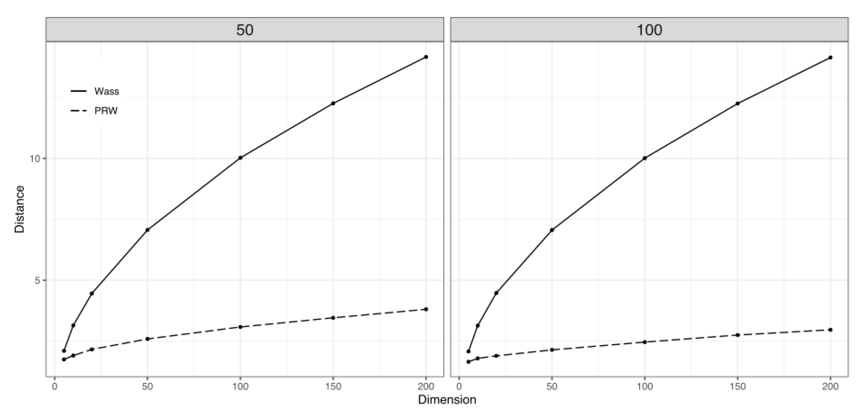
  • Compute the sample mean and sample covariance for each P d 0 , P d 1 , P d 2 , , P d 365 . Then, use these estimates to calculate the PRW distance, as defined in (20), between each P d i and the basis P d 0 . We denote these distances as G d 1 , G d 2 , , G d 365 . Note that calculating the Wasserstein distances directly is more time-consuming and may suffer from the curse of dimensionality if the number of assets is large, whereas the PRW distance does not. Additionally, since we choose δ using a backward selection approach, using the Wasserstein distance may result in a larger value of δ , leading to a more conservative MVP.
  • Select δ as the ( 1 ξ 0 ) th percentile of the empirical distribution of G d 1 , G d 2 , , G d 365 . The user-defined confidence level ξ 0 can be determined through cross-validation. In our empirical study, we found that choosing δ as the median of G d 1 , G d 2 , , G d 365 leads to better out-of-sample performance compared to selecting the minimum or maximum. However, users can try different percentile levels to find a more suitable value for δ . It is worth noting that since the distribution of G d depends on the choice of k, it is necessary to estimate k even when using cross-validation to determine δ .
Remark 1. 
Assuming bounded asset returns, let P be the unknown true distribution of returns with mean vector μ 0 and covariance matrix Σ 0 . Then, there exists a constant c > 1 that depends on P such that for any confidence level ξ 0 ( 0 , 1 ] , the sample mean μ T and sample covariance Σ T satisfy the concentration inequality P T ( μ 0 , Σ 0 ) U δ ( μ T , Σ T ) 1 ξ 0 whenever δ exceeds
δ T ( ξ 0 ) = log ( c / ξ 0 ) T .
Moreover, for all ξ 0 ( 0 , 1 ) and δ δ T ( ξ 0 ) , we have
P T ϕ Σ 0 ϕ max ( μ , Σ ) U δ ( μ T , Σ T ) ϕ Σ ϕ 1 ξ 0 ,
where ϕ is the optimal portfolio weight that solves the problem
max ( μ , Σ ) U δ ( μ T , Σ T ) 1 2 ϕ Σ ϕ     s . t .   ϕ μ = α .
Especially, if P is an elliptical distribution. Then,
max ( μ , Σ ) U δ ( μ T , Σ T ) ϕ Σ ϕ ϕ Σ 0 ϕ
almost surely as T .
Remark 1 provides a large sample performance guarantee for our approach, which is a direct result of Theorems 21, 22, and 23 in [25]. These theorems assert that the uncertainty set U δ ( μ , Σ ) with radius δ δ T ( ξ 0 ) represents a ( 1 ξ 0 ) confidence set for the mean and covariance of the population distribution P . The theorems also provide an upper confidence bound on the out-of-sample performance of the MVP that is constructed based on the training samples. For convergence rates in Wasserstein distance of the empirical measure, readers can refer to [26].
We conducted an experiment to test if using different covariance estimators would affect the empirical distribution of δ in high-dimensional settings. We iteratively generate asset returns R t N ( μ 0 , Σ ) for 500 times, where Σ is the sum of two positive definite matrices Σ 0 and Σ e , with Σ 0 having a low-rank structure and Σ e = L e L e . We randomly sample μ 0 and L e from N ( 0 , 1 ) . Table 1 displays the empirical distribution of δ using our method, which is based on the sample mean and three different covariance estimators: the sample covariance ( Σ s a m ) , the POET estimator ( Σ P O E T ) in [7], and the shrinkage estimator ( Σ L W ) in [27]. The empirical distribution of δ is robust to all listed covariance estimators, as shown in the table. We also conduct a Kolmogorov–Smirnov test on the distributions of δ ^ using the sample covariance, POET, and shrinkage estimators. The test fails to reject the null hypothesis that any two distributions are the same given N and T. Hence, we suggest simply using the sample mean and sample covariance to estimate δ in practice.

2.2.2. Methods for Choosing k

The topic of estimating the number of factors is important and has been extensively studied in the literature. Wang provided a survey of the methods and categorized them based on the asymptotic regimes of fixed N and T , and both N and T .
Under the regime of fixed N and T , various methods for estimating the number of factors have been compared, such as scree plot, Bartlett’s test, and cross-validation [28]. Ref. [29] further introduced percent variance, Kaiser test, parallel analysis (PA), and the minimum average partial procedure, and selected PA as the best approach due to its practical performance, although it assumes finite-dimensional data and lacks theoretical guarantees. PA is a method for estimating the number of factors, which involves comparing the rth factor to the 95th percentile of the rth eigenvalues of a simulated correlation matrix, for r = 1 , , N . If the rth factor is larger than the 95th percentile of the simulated rth factor, and all previous r 1 factors have been retained, then the rth factor is also retained. Originally, PA simulated the correlation matrix from a Gaussian distribution [30], but [31] introduced a permutation version of PA that shows better performance in simulations.
Under the regime of N , T while k is fixed, the existing methods to estimate the low-rank or the number of factors can be classified by assuming strong or weak factors. Strong factors correspond to significant loadings B, where B B / T Σ B , and include the methods of [32](BN), [33], and [34](AH). These methods typically use information criteria or eigengaps to estimate the number of factors. Compared to strong factors, weak factors assume B B Σ B instead of B B / T Σ B . Methods for estimating weak factors include [35,36] (KN), and [37]. These methods are designed for the case where the idiosyncratic components have homoscedastic noise ϵ = σ 2 I and factors have eigenvalues larger than σ 2 T / N when N , T , T / N c > 0 . It is known [36,38] that there exists a phase transition phenomenon. That is, the factors are not detectable if their associated eigenvalues are below some threshold, even for the homoscedastic noise ϵ = σ 2 I .

3. Monte Carlo Simulations

In this section, we describe our simulation experiments and discuss the comparison of different portfolio selection methods.

3.1. Setting

We simulate asset-returns from a normal distribution, N ( 0 , Σ ) , where Σ is the sum of the signal component Σ s and the noise component Σ e . The signal Σ s is defined as B C o v ( F ) B , where F are the Fama–French three factors, B are the corresponding factor loadings obtained by regressing the monthly returns of N = 82 S&P 100 index constituent stocks on F, and C o v ( F ) is the covariance matrix of F. The noise Σ e is obtained by applying the soft-thresholding approach in [39] on the sample covariance of the residuals from the regression.

3.2. Comparison of Methods of Choosing k

In this section, we suggest an approach from choosing the number of factors in Section 2.2.2. The estimation accuracy of k is known to depend on the relative magnitudes of Σ s and Σ e [37]. We thus generate returns from
R N ( 0 , Σ )     s . t .     Σ = Σ s Σ s + γ · Σ e Σ e .
The signal and noise were normalized to unity using their Frobenius norm, with a constant γ adjusting the signal and noise ratio. Four methods (PA, BN, AH, and KN) were compared for selecting the true number of factors in a dataset of 20 randomly chosen stocks with 200 observations per iteration. The true number of factors was 3, and the total iteration was 500. Table 2 shows the correct rank selection rate, with PA having the highest correct rate and outperforming the other methods when the noise was large. Therefore, PA is the preferred method.

3.3. Performance of Various GMVP Estimators

In this section, we compare various estimators for GMVP, including the BCZ method and our proposed approach. Specifically, we compare three GMVP estimators: w ^ ( Σ S a m ) , w ^ ( Σ P O E T ) , and w ^ ( Σ L W ) , which are estimated by plugging in w ^ ( Σ ) = Σ 1 1 1 Σ 1 1 with the sample covariance matrix Σ S a m , POET estimator Σ P O E T [7], the Ledoit–Wolf shrinkage estimator [27], and the equal-weight portfolio w ^ e w . Our proposed GMVP estimator is obtained by solving the following optimization problem:
w ^ D S R = argmin ϕ ϕ Var P T ( R ) ϕ + δ k ϕ 2   s . t .   ϕ 1 = 1 ,
where δ k is computed using the method introduced in Section 2.2.1. We highlight the advantage of using the projected robust Wasserstein (PRW) distance over the regular Wasserstein distance when the data dimension is large. Because there is only theoretical guidance for choosing δ based on large samples in the BCZ method, it is not clear how to compute δ using empirical data. The GMVP and minimum variance portfolio (MVP) estimates referred to in this paper using the BCZ method, denoted as w ^ D R , are computed in the same way as ours, except that δ is computed using the regular Wasserstein distance.
We allow for short positions in our portfolio weightings. The performance of the aforementioned methods is evaluated based on the risk ratio (R.R.), as defined in [8]:
R . R . = R ( w ^ ) R min = w ^ Σ w ^ w Σ w ,
where w = Σ 1 1 1 Σ 1 1 and w ^ are the GMVP estimators based on the generated returns, as introduced in Section 3.1. For both the BCZ and our proposed approaches, we estimate the empirical distributions of δ and δ k from the sampled returns, and select their 25 % , 50 % , and 75 % percentiles as the values of δ and δ k , respectively. We also consider the transaction cost (Trans) of all the listed portfolios, which is captured by the Euclidean norm of weight vectors. The results are reported in Table 3.
In Table 3, the values in parentheses ( · ) denote the standard deviations. We use the 25 % , 50 % , and 75 % percentiles of the empirical distribution of δ k to select the benchmark values for our GMVP estimator, and compare them with the other GMVP estimators. We employ a one-sided t-test with the null hypothesis:
H 0 : R . R . w ^ ( Σ ) < { R . R . w ^ D S R ( δ 25 % ) ,   R . R . w ^ D S R ( δ 50 % ) ,   R . R . w ^ D S R ( δ 75 % ) } .
The corresponding p-values are presented in square brackets in the form of [ · / · / · ] . As shown in the table, for all combinations of N , T in our experiment, w ^ D S R exhibits a lower R . R . than w ^ D R and w ^ e w . We observe that the GMVP estimates w ^ ( Σ P O E T ) and w ^ ( Σ L W ) , which are global variance minimizers, have a lower risk ratio ( R . R . ) than our w ^ D S R . However, this can be attributed to the fact that our w ^ D S R is estimated by minimizing the global variance plus a regularization term, while the other GMVP estimators do not include any additional terms in their objective functions. In contrast, w ^ ( Σ P O E T ) and w ^ ( Σ L W ) are pure global variance minimizers. It is important to note that our w ^ D S R enjoys a more robust out-of-sample performance than the other GMVP estimators, as we will show later, at the expense of sacrificing some sharp risk consistency, which is defined as R ( w ^ ) R min p 1 as T . This is because our estimator is designed to be more robust to model misspecification and market noise. Regarding transaction cost, w ^ ( Σ P O E T ) , w ^ ( Σ S a m ) , and w ^ ( Σ L W ) can be seen as δ = 0 , while w ^ e w can be seen as δ = . We find that larger values of the regularization parameter imply lower transaction costs.

3.4. Robustness of Various MVP Estimators

In this section, we compare the robustness of the Sharpe ratio of our DSR-MVP with other MVP estimators listed in the previous section. We use the same data generating process as in Section 3.1, but with a larger set of stocks ( N = 388 ) that remained in the S&P 500 index during the period 2001–2021. All MVPs were trained using the covariance Σ = Σ s + Σ e , with the required return set to be the same as that of the equal-weight portfolio. We compute the Sharpe ratios by averaging 500 iterations based on simulated returns from N ( μ , Σ ( a ) ) , where μ is a vector of average returns for each stock and Σ ( a ) = Σ s + a · Σ e . By tuning the value of a, we adjust the relative magnitude of the noise to the signal. The results are presented in Figure 2. Figure 2 shows that all MVPs have a lower Sharpe ratio when the returns are more noisy. However, our DSR-MVP enjoys the highest Sharpe ratio compared to the other MVPs across all levels of noise. The shadow areas represent the corresponding confidence intervals at a significance level of 5 % . We observe that even the lower boundary of the confidence interval for the Sharpe ratio of our DSR-MVP is higher than the average Sharpe ratio of the other MVPs.

4. Empirical Results

In this section, we evaluate the out-of-sample performance of our DSR-MVP estimator. We use the daily returns of the S&P 500 index span from 2001 to 2021. This gives us a sample of N = 388 stocks, with T = 5282 periods of observations.
We compared the performance of our DSR-MVP estimator with other MVP estimators using a rolling-out-of-sample testing approach. We trained the initial portfolios using data from 2001–2002, with a training set of 24 months that is updated each month by excluding the first month and adding the next month. This allows us to recalculate portfolio weights every month. We set the required return to be the same as the equal-weight portfolio. The performance of each portfolio are evaluated based on its out-of-sample annualized Sharpe ratio (S.R.) and risk. We used a testing set of one month of data, with the out-of-sample period spanning from 2003 to 2021, a total of 227 months.
To construct our DSR-MVP estimator, we first estimate the empirical distribution of δ using the approach introduced in Section 2.2.1. We use each training set as a block and estimate the mean and covariance using the daily returns from that block. We repeat this process for the remaining blocks, resulting in 228 pairs of ( μ ^ , Σ ^ ) denoted as ( μ ^ , Σ ^ ) 1 , ( μ ^ , Σ ^ ) 2 , , ( μ ^ , Σ ^ ) 228 . We choose ( μ ^ , Σ ^ ) 1 , which is estimated based on stock returns during 2001–2002 as the basis and compute the PRW distance between ( μ ^ , Σ ^ ) 1 and ( μ ^ , Σ ^ ) t using (20) for t = 2 , , 228 . This results in 227 PRW distances that measure the deviation of the distribution of a given block from the basis block. We plot the values of these PRW distances along with the S&P 500 index in Figure 3. Both curves were normalized by dividing their first values. From Figure 3, we can observe that the Gelbrich distances and the S&P 500 index have a reverse corresponding relationship. Although the former cannot be used to predict the rise and fall of the stock market, it can describe the difference between the stock market return distribution in a specified period and the base period. We estimate the empirical distribution of δ k from these PRW distances and set its median as the value of δ k to construct our DSR-MVP estimator. Practitioners can try using more percentiles for cross-validation.
Table 4 presents the annual risks and Sharpe ratios of the listed MVPs from 2003 to 2021. Both are computed by averaging their 12 monthly values for the year. We choose our w ^ D S R as the benchmark and conduct the following two-sided t-tests: H 0 : R i s k w ^ = R i s k w ^ D S R and H 0 : S . R . w ^ = S . R . w ^ D S R , where w ^ { w ^ ( Σ s a m ) , w ^ ( Σ P O E T ) , w ^ ( Σ W F ) , w ^ e w , w ^ D R } . In panel (a), our DSR-MVP exhibits a significantly lower risk than the traditional “plug-in” MVPs and the equal-weights portfolio for most of the years, indicating its clear advantage concerning out-of-sample risk. In panel (b), we must acknowledge that no single portfolio significantly dominates the others when using real market data without imposing any structures in terms of Sharpe ratio. However, this result can be interpreted as indicating that, with similar Sharpe ratio performance, our PRW-based DRO portfolio achieves lower risk than the classic “plug in” MVPs.

5. Conclusions

This paper introduces a new PRW distance-based DRO to the Markowitz portfolio selection. The main contribution is to enhance the existing DRO method proposed by BCZ with high-dimensional data. The application of the regular Wasserstein distance in BCZ may lead to an overly conservative strategy when managing a large number of assets. In contrast, our DRO method, which employs the PRW distance, concentrates solely on the principal components that account for most of the variability in asset returns. By focusing on the key factors, our approach mitigates the conservatism issue that arises when handling many assets. Our simulation results demonstrate that our DSR-MVP attains the highest Sharpe ratio in comparison to both conventional “plug-in” MVPs and DRO utilizing regular Wasserstein distance. This is especially evident when the data’s signal component has a low-rank structure and when the data is noisy. Our method provides practitioners with a comprehensive solution for estimating the optimal allocation policy based solely on asset return data without any exogenously given inputs. Furthermore, our empirical study indicates that the distributionally robust Wasserstein MVP outperforms conventional “plug-in” MVPs, in terms of lower risk, utilizing different covariance matrix estimators during out-of-sample testing. Future research can explore the connection between DRO problems and regularization in MVP using optimal transport discrepancy or other measures such as the phi-divergences, as discussed in [18]. Moreover, we find that estimating the number of latent factors consistently requires relatively strong factors. We also consider possible extensions to allow for weak factors, but formal theoretical studies on this issue are left for future work.

Author Contributions

Conceptualization, Z.Z.; methodology, Z.Z.; software, Z.Z. and H.J.; formal analysis, Z.Z.; writing—original draft preparation, Z.Z.; writing—review and editing, Z.Z., H.J. and C.K.; visualization, H.J.; supervision, C.K. All authors have read and agreed to the published version of the manuscript.

Funding

This research received no external funding.

Institutional Review Board Statement

Not applicable.

Informed Consent Statement

Not applicable.

Data Availability Statement

The data presented in this study are openly available in Yahoo Finance.

Conflicts of Interest

The authors declare no conflict of interest.

References

  1. Markowitz, H. Portfolio Selection. J. Financ. 1952, 7, 77–91. [Google Scholar]
  2. DeMiguel, V.; Nogales, F.J. Portfolio Selection with Robust Estimation. Oper. Res. 2009, 57, 560–577. [Google Scholar] [CrossRef] [Green Version]
  3. Michaud, R.O. The Markowitz Optimization Enigma: Is ’Optimized’ Optimal? Financ. Anal. J. 1989, 45, 31–42. [Google Scholar] [CrossRef]
  4. DeMiguel, V.; Garlappi, L.; Uppal, R. Optimal Versus Naive Diversification: How Inefficient is the 1-N Portfolio Strategy? Rev. Financ. Stud. 2009, 22, 1915–1953. [Google Scholar] [CrossRef] [Green Version]
  5. Merton, R.C. On estimating the expected return on the market: An exploratory investigation. J. Financ. Econ. 1980, 8, 323–361. [Google Scholar] [CrossRef]
  6. Jagannathan, R.; Ma, T. Risk Reduction in Large Portfolios: Why Imposing the Wrong Constraints Helps. J. Financ. 2003, 58, 1651–1683. [Google Scholar] [CrossRef] [Green Version]
  7. Fan, J.; Liao, Y.; Mincheva, M. Large covariance estimation by thresholding principal orthogonal complements. J. R. Stat. Soc. Ser. B (Stat. Methodol.) 2013, 75, 603–680. [Google Scholar] [CrossRef] [PubMed] [Green Version]
  8. Ding, Y.; Li, Y.; Zheng, X. High dimensional minimum variance portfolio estimation under statistical factor models. J. Econom. 2021, 222, 502–515. [Google Scholar] [CrossRef]
  9. Cai, T.T.; Hu, J.; Li, Y.; Zheng, X. High-dimensional minimum variance portfolio estimation based on high-frequency data. J. Econom. 2020, 214, 482–494. [Google Scholar] [CrossRef]
  10. Ledoit, O.; Wolf, M. Improved estimation of the covariance matrix of stock returns with an application to portfolio selection. J. Empir. Financ. 2003, 10, 603–621. [Google Scholar] [CrossRef] [Green Version]
  11. Ledoit, O.; Wolf, M. A well-conditioned estimator for large-dimensional covariance matrices. J. Multivar. Anal. 2004, 88, 365–411. [Google Scholar] [CrossRef] [Green Version]
  12. Ledoit, O.; Wolf, M. Nonlinear Shrinkage of the Covariance Matrix for Portfolio Selection: Markowitz Meets Goldilocks. Rev. Financ. Stud. 2017, 30, 4349–4388. [Google Scholar] [CrossRef] [Green Version]
  13. Huber, P.J. Robust Estimation of a Location Parameter. Ann. Math. Stat. 1964, 35, 73–101. [Google Scholar] [CrossRef]
  14. Hampel, F. Contributions to the Theory of Robust Estimation; University Microfilms: Ann Arbor, MI, USA, 1976. [Google Scholar]
  15. Perret-Gentil, C.; Victoria-Feser, M.P. Robust Mean-Variance Portfolio Selection. SSRN Electron. J. 2007. [Google Scholar] [CrossRef] [Green Version]
  16. Scarf, H. A Min-Max Solution of an Inventory Problem. In Studies in the Mathematical Theory of Inventory and Production; Rand Corporation: Santa Monica, CA, USA, 1958; pp. 201–209. [Google Scholar]
  17. Blanchet, J.; Chen, L.; Zhou, X.Y. Distributionally Robust Mean-Variance Portfolio Selection with Wasserstein Distances. Manag. Sci. 2022, 68, 6382–6410. [Google Scholar] [CrossRef]
  18. DeMiguel, V.; Garlappi, L.; Nogales, F.J.; Uppal, R. A Generalized Approach to Portfolio Optimization: Improving Performance by Constraining Portfolio Norms. Manag. Sci. 2009, 55, 798–812. [Google Scholar] [CrossRef] [Green Version]
  19. Olivares-Nadal, A.V.; DeMiguel, V. Technical Note—A Robust Perspective on Transaction Costs in Portfolio Optimization. Oper. Res. 2018, 66, 733–739. [Google Scholar] [CrossRef]
  20. Esfahani, M.P.; Kuhn, D. Data-driven distributionally robust optimization using the Wasserstein metric: Performance guarantees and tractable reformulations. Math. Program. 2018, 171, 115–166. [Google Scholar] [CrossRef] [Green Version]
  21. Lin, T.; Fan, C.; Ho, N.; Cuturi, M.; Jordan, M.I. Projection Robust Wasserstein Distance and Riemannian Optimization. Adv. Neural Inf. Process. Syst. 2020, 33, 9383–9397. [Google Scholar]
  22. Paty, F.P.; Cuturi, M. Subspace Robust Wasserstein Distances. In Proceedings of the International Conference on Machine Learning, Long Beach, CA, USA, 9–15 June 2019; pp. 5072–5081. [Google Scholar]
  23. Deshpande, I.; Hu, Y.T.; Sun, R.; Pyrros, A.; Siddiqui, N.; Koyejo, S.; Zhao, Z.; Forsyth, D.; Schwing, A. Max-Sliced Wasserstein Distance and its use for GANs. In Proceedings of the IEEE/CVF Conference on Computer Vision and Pattern Recognition, Long Beach, CA, USA, 16–20 June 2019; pp. 10648–10656. [Google Scholar]
  24. Nguyen, K.; Ho, N.; Pham, T.; Bui, H. Distributional Sliced-Wasserstein and Applications to Generative Modeling. arXiv 2020, arXiv:2002.07367. [Google Scholar]
  25. Kuhn, D.; Esfahani, P.M.; Nguyen, V.A.; Shafieezadeh-Abadeh, S. Wasserstein Distributionally Robust Optimization: Theory and Applications in Machine Learning. In Operations Research & Management Science in the Age of Analytics; Informs: Catonsville, MD, USA, 2019. [Google Scholar]
  26. Fournier, N.; Guillin, A. On the rate of convergence in Wasserstein distance of the empirical measure. Probab. Theory Relat. Fields 2015, 162, 707–738. [Google Scholar] [CrossRef] [Green Version]
  27. Ledoit, O.; Wolf, M. Spectrum estimation: A unified framework for covariance matrix estimation and PCA in large dimensions. J. Multivar. Anal. 2015, 139, 360–384. [Google Scholar] [CrossRef]
  28. Jolliffe, I.T. Principal Component Analysi; Springer: Berlin, Germany, 2002. [Google Scholar]
  29. Velicer, W.F.; Eaton, C.A.; Fava, J.L. Construct Explication through Factor or Component Analysis: A Review and Evaluation of Alternative Procedures for Determining the Number of Factors or Components. In Problems and Solutions in Human Assessment: Honoring Douglas N. Jackson at Seventy; Springer US: Boston, MA, USA, 2000; Chapter 3; pp. 41–71. [Google Scholar]
  30. Horn, J. A rationale and test for the number of factors in factor analysis. Psychometrika 1965, 30, 179–185. [Google Scholar] [CrossRef] [PubMed]
  31. Buja, A.; Eyuboglu, N. Remarks on Parallel Analysis. Multivar. Behav. Res. 1992, 27, 509–540. [Google Scholar] [CrossRef] [PubMed]
  32. Bai, J.; Ng, S. Determining the Number of Factors in Approximate Factor Models. Econometrica 2002, 70, 191–221. [Google Scholar] [CrossRef] [Green Version]
  33. Onatski, A. Determining the Number of Factors from Empirical Distribution of Eigenvalues. Rev. Econ. Stat. 2010, 92, 1004–1016. [Google Scholar] [CrossRef]
  34. Ahn, S.C.; Horenstein, A.R. Eigenvalue Ratio Test for the Number of Factors. Econometrica 2013, 81, 1203–1227. [Google Scholar] [CrossRef]
  35. Muirhead, R.J. Latent Roots and Matrix Variates: A Review of Some Asymptotic Results. Ann. Statist. 1978, 6, 5–33. [Google Scholar] [CrossRef]
  36. Kritchman, S.; Nadler, B. Non-Parametric Detection of the Number of Signals: Hypothesis Testing and Random Matrix Theory. IEEE Trans. Signal Process. 2009, 57, 3930–3941. [Google Scholar] [CrossRef]
  37. Choi, Y.; Taylor, J.; Tibshirani, R. Selecting the number of principal components: Estimation of the true rank of a noisy matrix. Ann. Statist. 2017, 45, 2590–2617. [Google Scholar] [CrossRef]
  38. Wang, J. Factor Analysis For High-dimensional Data. Ph.D. Thesis, Stanford University, Stanford, CA, USA, 2016. [Google Scholar]
  39. Rothman, A.J. Positive definite estimators of large covariance matrices. Biometrika 2012, 99, 733–740. [Google Scholar] [CrossRef]
Figure 1. Various type of Wasserstein distances depending on the dimension N.
Mathematics 11 01272 g001
Figure 2. Sharpe ratio of various MVPs under noisy returns.
Mathematics 11 01272 g002
Figure 3. Gelbrich distances and S&P 100 index during 2003–2021.
Mathematics 11 01272 g003
Table 1. Empirical distribution of δ ^ based on various estimators of covariance.
Percentile of δ KS Test (p-Value)
N T Estimatormin25%50%75%maxH1H2H3
50100 δ ^ ( Σ s a m ) 1.262.6173.2243.9688.886N = 50, T = 100
50100 δ ^ ( Σ P O E T ) 1.2982.6393.2163.9828.89710.7180.770
50100 δ ^ ( Σ L W ) 1.0592.6823.2914.0158.851
100100 δ ^ ( Σ s a m ) 1.6143.6854.5315.5510.382N = 100, T = 100
100100 δ ^ ( Σ P O E T ) 1.6483.6544.5495.54910.46010.7400.614
100100 δ ^ ( Σ L W ) 1.6053.7914.6435.6149.945
200100 δ ^ ( Σ s a m ) 2.4995.196.47.69814.395N = 200, T = 100
200100 δ ^ ( Σ P O E T ) 2.4465.1576.3887.68114.36410.3990.356
200100 δ ^ ( Σ L W ) 2.2655.3846.5697.76315.088
H1: δ ^ ( Σ s a m ) and δ ^ ( Σ P O E T ) follow same distribution. H2: δ ^ ( Σ s a m ) and δ ^ ( Σ L W ) follow same distribution. H3: δ ^ ( Σ P O E T ) and δ ^ ( Σ L W ) follow same distribution.
Table 2. Correct rate using various methods of choosing k.
γ BNAHPAKN γ BNAHPAKN
0.030.0620.520.94200.180.3400.760
0.060.120.0660.91400.210.37200.6580
0.090.1160.0040.91200.240.3900.60
0.120.22400.88600.270.38600.5140
0.150.25600.81800.300.37400.4360
Table 3. Comparison of various GMVP estimators.
N = 83 , T = 50
Choice of δ
R.R.p-valueTrans 25%50%75%
w ^ ( Σ S a m ) 2.703 (0.349)[0/0/0]0.466 (0.117) w ^ D R R.R.5.689 (3.472) [0]6.396 (3.991) [0]7.757 (4.893) [0]
w ^ ( Σ P O E T ) 1.382 (0.066)[1/1/1]0.105 (0.004) Trans0.073 (0.01)0.07 (0.011)0.066 (0.012)
w ^ ( Σ L W ) 1.331 (0.065)[1/1/1]0.102 (0.004) w ^ D S R R.R.2.067 (0.363)2.174 (0.437)2.429 (0.629)
w ^ ( Σ e w ) 9.926 (-)[0/0/0]0.012 (-) Trans0.1 (0.005)0.097 (0.005)0.093 (0.006)
N = 83 , T = 100
Choice of δ
R.R.p-valueTrans 25%50%75%
w ^ ( Σ S a m ) 2.362 (0.365)[0/0/0]0.577 (0.18) w ^ D R R.R.2.278 (0.369) [0]2.354 (0.402) [0]2.516 (0.473) [0]
w ^ ( Σ P O E T ) 1.313 (0.029)[1/1/1]0.104 (0.003) Trans0.09 (0.004)0.089 (0.004)0.087 (0.004)
w ^ ( Σ L W ) 1.237 (0.03)[1/1/1]0.109 (0.003) w ^ D S R R.R.1.717 (0.151)1.772 (0.171)1.861 (0.204)
w ^ ( Σ e w ) 9.926 (-)[0/0/0]0.012 (-) Trans0.102 (0.003)0.1 (0.003)0.097 (0.003)
N = 83 , T = 100
Choice of δ
R.R.p-valueTrans 25%50%75%
w ^ ( Σ S a m ) 1.3 (0.054)[1/1/1]0.227 (0.024) w ^ D R R.R.1.699 (0.112) [0]1.725 (0.118) [0]1.783 (0.131) [0]
w ^ ( Σ P O E T ) 1.285 (0.017)[1/1/1]0.104 (0.002) Trans0.097 (0.002)0.097 (0.002)0.095 (0.002)
w ^ ( Σ L W ) 1.158 (0.021)[1/1/1]0.125 (0.006) w ^ D S R R.R.1.519 (0.074)1.545 (0.079)1.597 (0.09)
w ^ ( Σ e w ) 9.926 (-)[0/0/0]0.012 (-) Trans0.103 (0.002)0.102 (0.002)0.1 (0.002)
p-value 0 implies that p > 0.001 and p-value 1 implies that p > 0.999.
Table 4. Performance of various MVP estimators using empirical data.
(a) Risk
Year w ^ ( Σ sam ) w ^ ( Σ POET ) w ^ ( Σ WF ) w ^ ew w ^ DR w ^ DSR
20033.23 ***2.50 *2.154.64 ***2.142.10
20043.27 ***3.31 ***2.363.59 ***2.462.35
20053.18 ***3.07 ***2.103.31 ***2.42.12
20063.32 ***2.53 ***1.903.31 ***2.011.91
20073.64 ***3.16 *2.314.51 ***2.912.33
20086.79 *6.534.4910.81 ***4.634.51
20096.25 ***5.62 **3.608.59 ***3.433.71
20104.08 ***2.672.565.23 ***2.562.49
20113.86 **3.112.666.49 ***2.982.70
20123.67 ***2.53 ***2.053.79 ***1.942.01
20133.46 ***2.92 **2.393.35 ***2.452.35
20143.32 ***3.39 ***2.123.11 **2.512.15
20153.97 **4.81 ***3.024.15 **3.633.09
20164.73 ***5.6 ***2.733.842.792.56
20174.09 ***2.78 ***2.12 **1.991.641.81
20184.58 ***4.13 **3.064.01 *3.313.00
20194.42 ***3.74 ***2.543.25 **2.362.32
20208.56 *8.86 *5.558.535.735.59
20215.64 ***4.94 ***3.043.83 ***2.72.98
(b) Sharpe Ratio
Year w ^ ( Σ sam ) w ^ ( Σ POET ) w ^ ( Σ WF ) w ^ ew w ^ DR w ^ DSR
20030.54 *0.751.150.951.241.21
20040.880.881.200.721.051.01
20050.170.320.290.530.480.35
20060.160.680.760.700.820.78
20070.200.310.350.390.470.44
2008−0.05−0.21−0.11−0.01−0.13−0.12
2009−0.260.130.230.650.230.09
20100.480.480.490.760.570.50
20110.550.860.460.260.530.52
20120.240.120.400.610.360.41
20130.870.650.671.010.890.72
20140.490.640.830.720.820.87
20150.320.440.50.290.350.49
20160.000.080.480.600.450.57
20170.060.390.491.140.940.63
20180.090.470.330.340.510.46
20190.520.551.101.071.091.05
20200.22−0.080.100.520.290.12
20210.10 *0.290.730.740.720.76
Significant. codes: 0 ‘***’ 0.001 ‘**’ 0.01 ‘*’ 0.05 ‘.’ 0.1 ‘ ’ 1.
Disclaimer/Publisher’s Note: The statements, opinions and data contained in all publications are solely those of the individual author(s) and contributor(s) and not of MDPI and/or the editor(s). MDPI and/or the editor(s) disclaim responsibility for any injury to people or property resulting from any ideas, methods, instructions or products referred to in the content.

