On Horadam Sequences with Dense Orbits and Pseudo-Random Number Generators

Abstract

Horadam sequence is a general recurrence of second order in the complex plane, depending on four complex parameters (two initial values and two recurrence coefficients). These sequences have been investigated over more than 60 years, but new properties and applications are still being discovered. Small parameter variations may dramatically impact the sequence orbits, generating numerous patterns: periodic, convergent, divergent, or dense within one dimensional curves. Here we explore Horadam sequences whose orbit is dense within a 2D region of the complex plane, while the complex argument is uniformly distributed in an interval. This enables the design of a pseudo-random number generator (PRNG) for the uniform distribution, for which we test periodicity, correlation, Monte Carlo estimation of $\pi$, and the NIST battery of tests. We then calculate the probability distribution of the radii of the sequence terms of Horadam sequences. Finally, we propose extensions of these results for generalized Horadam sequences of third order.

1. Introduction

Let $a,b,p,q$ be arbitrary complex numbers. The sequence defined by the relation

$$\begin{array}{cc}\hfill w_n& =p{w}_{n-1}+q{w}_{n-2}(n\ge 2),\hfill \\ \hfill w_0& =a,w_1=b,\hfill \end{array}$$

(1)

is often called a Horadam sequence ${\left(w_n\right)}_{n\ge 0}$, after Alwyn F. Horadam who initiated the detailed investigations regarding this sequence in the 1960s [1,2,3], establishing a great number of identities, properties, and generalizations.

At the time when it was formulated in this way by Horadam, this sequence had a significant impact, bridging the gap between the classical sequences studied by Édouard Lucas, and the application of many techniques from the special functions of mathematical physics [4]. Many of the results, new concepts and applications inspired by this research direction over sixty years have been summarised in a number of review papers, such as for example those by Larcombe et al. [5], or the update by Larcombe [6].

Numerous generalizations of the Horadam sequences have been investigated by many authors, as for example the k-Horadam introduced in 2012 by Yazlik [7] was recently applied to coding theory by Srividhya and Rani [8], or the bi-periodic Horadam sequence studied by Anđelić et al. [9], in relation to perturbed Toeplitz matrices (themselves used to enumerate the P-vertices of graphs [10]). Other related results and further properties can be found in classical or more recent papers [11,12,13,14,15,16].

Many classical integer sequences are obtained as particular cases: Fibonacci numbers for $(a,b)=(0,1)$ and $(p,q)=(1,1)$, Lucas numbers for $(a,b)=(2,1)$ and $(p,q)=(1,1)$, while Pell numbers for $(a,b)=(0,1)$ and $(p,q)=(2,1)$. These sequences (and over $\mathrm{350,000}$ others) are included in the On-Line Encyclopedia of Integer Sequences (OEIS) [17], together with numerous properties and applications [18]. As opposed to such classical integer sequences which are traditionally investigated via their algebraic or combinatorial properties, the orbits of complex Horadam sequences can be plotted in the complex plane, to produce a multitude of interesting geometric patterns.

The Horadam sequence terms defined by the recurrence (1) can be written explicitly using the zeros $z_1$, $z_2$ of the quadratic characteristic polynomial $P\left(x\right)=x^2-px-q$, called generators. These are linked to p and q by Vieta’s relations $p=z_1+z_2$ and $q=-z_1{z}_2$, and when $z_1\ne z_2$ one has

$$\begin{array}{c}\hfill w_n=A{z}_1^n+B{z}_2^n,\end{array}$$

(2)

where A and B calculated from the initial conditions are given by

$$\begin{array}{c}\hfill A=\frac{a{z}_2-b}{z_2-z_1},B=\frac{b-a{z}_1}{z_2-z_1}.\end{array}$$

(3)

This formulation allowed elegant characterization [19] (and enumeration) of periodic Horadam orbits, obtained when $z_1=e^{2\pi i{p}_1/k_1}$ and $z_2=e^{2\pi i{p}_2/k_2}$ are distinct roots of unity, with $p_1,p_2,k_1,k_2$ natural numbers. These have been enumerated in [20], while the dual symmetry was studied in [21]. Non-periodic Horadam patterns were presented in ([22], Chapter 5), with numerous examples of orbits dense within one-dimensional curves, or bi-dimensional regions of the complex plane, along with the sequence of ratios [23].

A natural but less commonly studied generalization is represented by the third-order Horadam sequences, defined by the relation

$$\begin{array}{cc}\hfill w_n& =p{w}_{n-1}+q{w}_{n-2}+r{w}_{n-3},(n\ge 3)\hfill \\ \hfill w_0& =a,w_1=b,w_2=c,\hfill \end{array}$$

(4)

where $a,b,c$ and $p,q,r$ are arbitrary complex numbers. Explicit formulae, properties, and geometric patterns for these sequences are given in ([22], Chapter 6.4) and [24,25].

Certain particular non-periodic dense Horadam patterns ($\left|A\right|=\left|B\right|$) were used by Bagdasar and Chen in the design of a novel pseudo-random number generator (PNRG) which performed well against other algorithms [26]. A proof of the uniformity of the complex argument of classical Horadam sequences was provided in ([22], Chapter 5.7).

Random number generators play an important role in many practical algorithms for statistical sampling or simulation. An illustrative application is the numerical solution of complicated integrals via Monte Carlo methods. As the convergence rate of a numerical algorithm is dependent on the characteristics of a distribution, one would ideally draw samples from a probability distribution resembling the underlying processes. Some of the common PRNG implementations involve Linear Congruences or Lagged Fibonacci Sequences (see, e.g., [27,28]). Other modern approaches employ ratios of integers [29], while the performance of PNRGs is usually tested against including period, uniformity and correlation [30], Monte Carlo simulations, or by statistical tests, such as NIST published by the National Institute of Standards and Technology [31], detailed in [32].

In this paper we study certain Horadam sequences of second and third order whose orbits is dense within a two-dimensional region of the complex plane, representing an annulus between two circles centred in the origin, of radii

$$\left|\right|A|-\left|B\right||=R_1<R_2=\left|A\right|+\left|B\right|,$$

with A, B given by (3). The sequence of complex arguments in these cases located the interval $[-\pi ,\pi ]$ is scaled to the interval $[0,1]$ and tested as a PRNG for the uniform distribution over this interval.

For this PRNG we will explore the period, uniformity, correlation, and approximate the value of $\pi$ using Monte Carlo simulations (contrasting the performance of this algorithms against that of some classical pseudo-random number generators), and also evaluate the results from NIST. We extend the results from [26] (where apart from some simulations, proofs were only provided for the particular case $\left|A\right|=\left|B\right|$) and ([22], Chapter 5.7) (where the theory for the arguments when $\left|A\right|\ne \left|B\right|$ was formulated). Additionally, we investigate for the first time the probability density for the sequence of radii of Horadam sequence terms, proving that generalized Horadam sequences of third-order and higher are also densely distributed within a circle of known radius.

The structure of the paper is as follows. Section 2 is dedicated to methodology, where we present basic properties of the (generalized) Horadam sequences, linear independence results, dense Horadam orbits, and PNRG testing. The performance of two PNRGs based on complex arguments of Horadam sequences is evaluated in Section 3 ($\left|A\right|=\left|B\right|$) and Section 4 ($\left|A\right|\ne \left|B\right|$). A similar study is carried out for third-order Horadam sequences in Section 5, while the probability density of the radii is discussed in Section 6. We end with some suggestions for further research.

2. Methodology

In this section we first discuss some basic notations, and establish the geometric bounds of periodic and stable orbits of Horadam sequences. We then present some density and uniformity results, and finally we give basic information about the testing of pseudo-random number generators. The graphs in this paper have been generated in Matlab^®, with the PRNG testing implemented in Python.

2.1. Geometric Properties of Horadam Sequences

For convenience we will use the notations

$$\begin{array}{cc}\hfill S& =S(0;1)=\{z\in \mathbb{C}\mid |z|=1\},S(z_0;r)=\{z\in \mathbb{C}\mid |z-z_0|=r\}\hfill \\ \hfill U& =U(0;1)=\{z\in \mathbb{C}\mid |z|<1\},U(z_0;r)=\{z\in \mathbb{C}\mid |z-z_0|<r\}\hfill \\ \hfill U(0;r_1,r_2)& =\{z\in \mathbb{C}\mid r_1<|z|<r_2\}.\hfill \end{array}$$

for the unit circle, the unit disc, and for the annulus of radii $r_1<r_2$ centered in the origin. For $z_1\ne z_2$, the orbit of the Horadam sequence ${\left(w_n\right)}_{n\ge 0}$ given by (2) will:

• Converge when $max\left\{\right|z_1|,|z_2\left|\right\}<1$,
• Diverge when $max\left\{\right|z_1|,|z_2\left|\right\}>1$,
• Be stable when $max\left\{\right|z_1|,|z_2\left|\right\}=1$.

When $|z_1|=|z_2|=1$, the resulting Horadam orbit (including periodic) satisfies

$$\begin{array}{c}\hfill U(0;|\left|A\right|-\left|B\right||,|A|+|B\left|\right)=\{z\in \mathbb{C}\mid |\left|A\right|-\left|B\right||\le |z|\le |A|+|B\left|\right\}.\end{array}$$

(5)

These boundaries represent an important feature of the Horadam orbits and are closely related to the probability density functions.

2.2. Linear Independence, Density and Uniform Distributions

We here present results on linear independence over $\mathbb{Q}$, density of sequences, and PRNG testing. Denote by $\lfloor x\rfloor =max\{m\in \mathbb{Z}\mid m\le x\}$ and $\left\{x\right\}=x-\lfloor x\rfloor$ the floor and fractional parts of x (this is periodic, satisfying $\{x+1\}=\left\{x\right\}$, $x\in \mathbb{R}$), respectively.

Definition 1. 

For $k\ge 1$, it is said that the numbers $x_1,\dots ,x_k\in \mathbb{R}$ are linearly dependent over $\mathbb{Q}$ (or $\mathbb{Z}$) if there are $p_1,\dots ,p_k\in \mathbb{Q}$, satisfying

$$\begin{array}{c}\hfill a_1{x}_1+a_2{x}_2+\dots +a_k{x}_k=0,\mathrm{and}(a_1,\dots ,a_k)\ne (0,\dots ,0).\end{array}$$

(6)

If (6) only holds for $(a_1,\dots ,a_k)=(0,\dots ,0)$, then $x_1,\dots ,x_k$ are called linearly independent.

Example 1. 

For $k=2$, when 1 and $x_1$ are linear independent, $x_1\in \mathbb{R}\setminus \mathbb{Q}$. For $k=3$, if p is prime, then $(1,\sqrt[3]{p},\sqrt[3]{p^2})$ is linearly independent over $\mathbb{Z}$. Clearly, $x_1,\dots ,x_k$ are linearly dependent over $\mathbb{Q}$, if and only if they are linearly dependent over $\mathbb{Z}$.

We now recall some well-known density results by Kronecker and Weyl.

Theorem 1 

(Theorem 339, [33]). If x is irrational, then ${\left(\left\{nx\right\}\right)}_{n\ge 0}$ is dense in $[0,1]$.

This result was further generalized by Weyl (see also ([33], Theorem 445)).

Theorem 2 

(Weyl, [34]). If x is irrational, then the sequence ${\left(\left\{nx\right\}\right)}_{n\ge 0}$, $n\in \mathbb{N}$ is uniformly distributed in $[0,1]$.

Kronecker’s lemma has the following extension to higher dimensions.

Theorem 3 

(Theorem 443, [33]). If $k\ge 2$ and $1,x_1,x_2\dots ,x_k$ are linearly independent, then the sequence ${(\left\{n{x}_1\right\},\left\{n{x}_2\right\},\dots ,\left\{n{x}_k\right\})}_{n\ge 0}$ is dense in the unit hypercube ${[0,1]}^k$.

In particular, when $k=2$ and $k=3$ the following results are obtained.

Proposition 1. 

Let $x_1,x_2\in \mathbb{R}$. If $(1,x_1,x_2)$ are linearly independent over $\mathbb{Q}$, then the sequence ${\left(\left\{n{x}_1\right\},\left\{n{x}_2\right\}\right)}_{n\ge 0}$ is dense within the unit square $[0,1]\times [0,1]$.

Proposition 2. 

Let $x_1,x_2,x_3\in \mathbb{R}$. If $(1,x_1,x_2,x_3)$ are linearly independent over $\mathbb{Q}$, then the sequence ${\left(\left\{n{x}_1\right\},\left\{n{x}_2\right\},\left\{n{x}_3\right\}\right)}_{n\ge 0}$ is dense within the unit cube $[0,1]\times [0,1]\times [0,1]$.

2.3. Dense Horadam Orbits

The dimension of the closure of Horadam orbits can be zero (for periodic, convergent, or divergent orbits), one (orbits dense within closed curves), or two (in which case the orbits are dense in the region between two circles centered in the origin).

Based on Section 2.1, the orbits are stable (neither convergent, nor divergent), so one has $|z_1|=|z_2|=1$. For convenience, the generators $z_1$, $z_2$ and the coefficients A and B given by (3) will be parametrised as

$$\begin{array}{c}\hfill z_1=e^{2\pi i{x}_1},z_2=e^{2\pi i{x}_2},A=R_1{e}^{i{\varphi }_1},B=R_2{e}^{i{\varphi }_2}.\end{array}$$

(7)

The terms $w_n$ of the Horadam sequence are given in polar form by

$$\begin{array}{c}\hfill w_n=r_n{e}^{i{\theta }_n}=A{z}_1^n+B{z}_2^n=R_1{e}^{i({\varphi }_1+2\pi n{x}_1)}+R_2{e}^{i({\varphi }_2+2\pi n{x}_2)},\end{array}$$

(8)

where $x_1$, $x_2$, ${\varphi }_1$, ${\varphi }_2$, $R_1$, $R_2$ and ${\theta }_n$, $r_n$ ($n\ge 0$) are real numbers, with $R_1,R_2,r_n\ge 0$.

The condition below ensures that the orbits are dense within a 2D region.

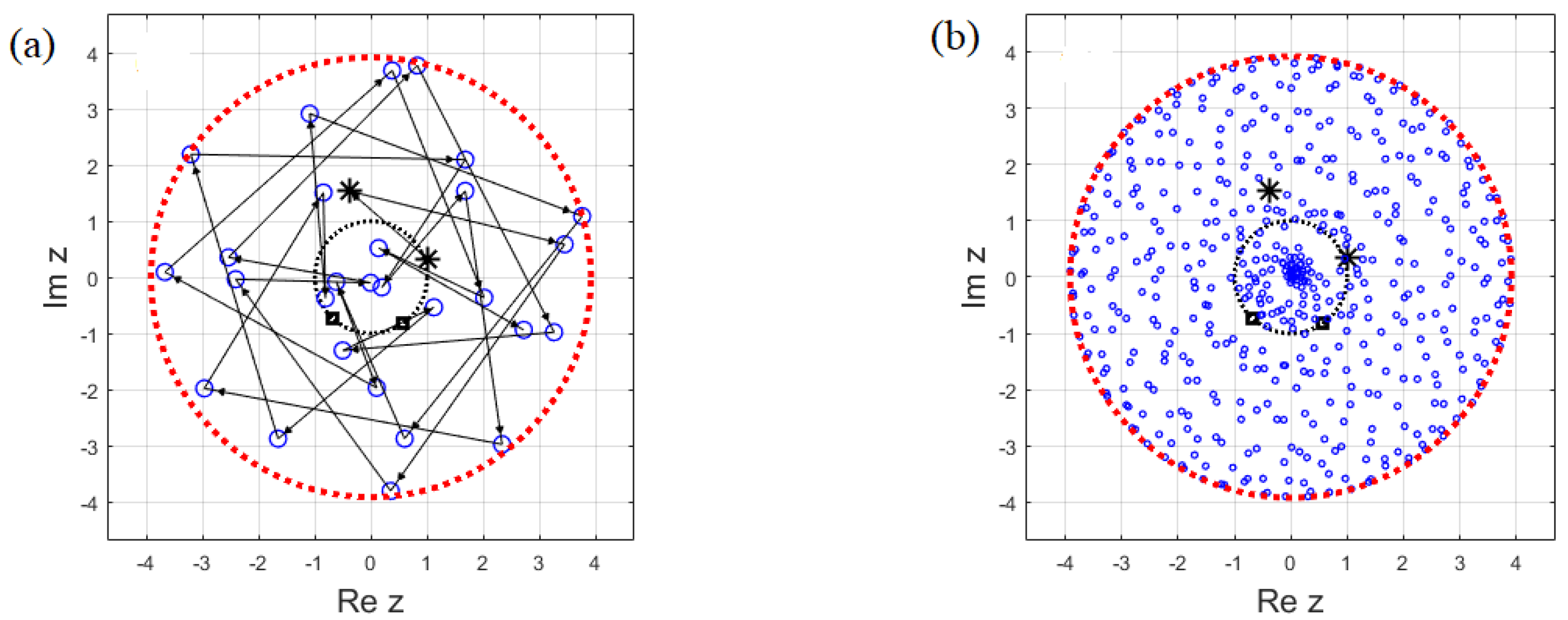
Theorem 4. 

Let $a,b\in \mathbb{C}$ and $x_1,x_2\in \mathbb{R}$. If $1,x_1,x_2$ are linearly independent over $\mathbb{Q}$, then the Horadam sequence with generators $z_1=e^{2\pi i{x}_1}\ne z_2=e^{2\pi i{x}_2}$ and seeds $w_0=a$ and $w_1=b$ is dense in the set $U(0;|\left|A\right|-\left|B\right||,|A|+|B\left|\right)$, with A and B computed by Formula (3).

Proof. 

We show that Horadam sequence terms can become arbitrarily close to an arbitrary point $w^{*}=r{e}^{i\theta }$ in the interior of the annulus $U(0;|R_1-R_2|,R_1+R_2)$. First, notice that there exist real numbers ${\theta }_1$ and ${\theta }_2$ satisfying

$$\begin{array}{c}\hfill w^{*}=r{e}^{i\theta }=R_1{e}^{i({\varphi }_1+2\pi {\phi }_1)}+R_2{e}^{i({\varphi }_2+2\pi {\phi }_2)}.\end{array}$$

(9)

Indeed, this can be proved by the identity

$$U(0;R_1)\oplus U(0;R_2)=U(0;|R_1-R_2|,R_1+R_2),$$

where ⊕ is the Minkovski sum of two sets.

We now prove that there is $w_n$ sufficiently close to $w^{*}$, i.e., for $\epsilon >0$ there is a natural number n such that $|w_n-w^{*}|<\epsilon$. By the continuity of the functions involved, this holds if one can find n such that $|n{x}_1-{\phi }_1|<\delta$ and $|n{x}_2-{\phi }_2|<\delta$, for a small $\delta >0$.

Since $(1,x_1,x_2)$ are linearly independent over $\mathbb{Q}$, by Proposition 1 the sequence ${\left(\left\{n{x}_1\right\},\left\{n{x}_2\right\}\right)}_{n\ge 0}$ is dense within $[0,1]\times [0,1]$, so there are terms $w_n$ arbitrarily close to $w^{*}$, i.e., the sequence ${\left(w_n\right)}_{n\ge 0}$ is dense in the annulus $U(0,|\left|A\right|-\left|B\right||,|A|+|B\left|\right)$. □

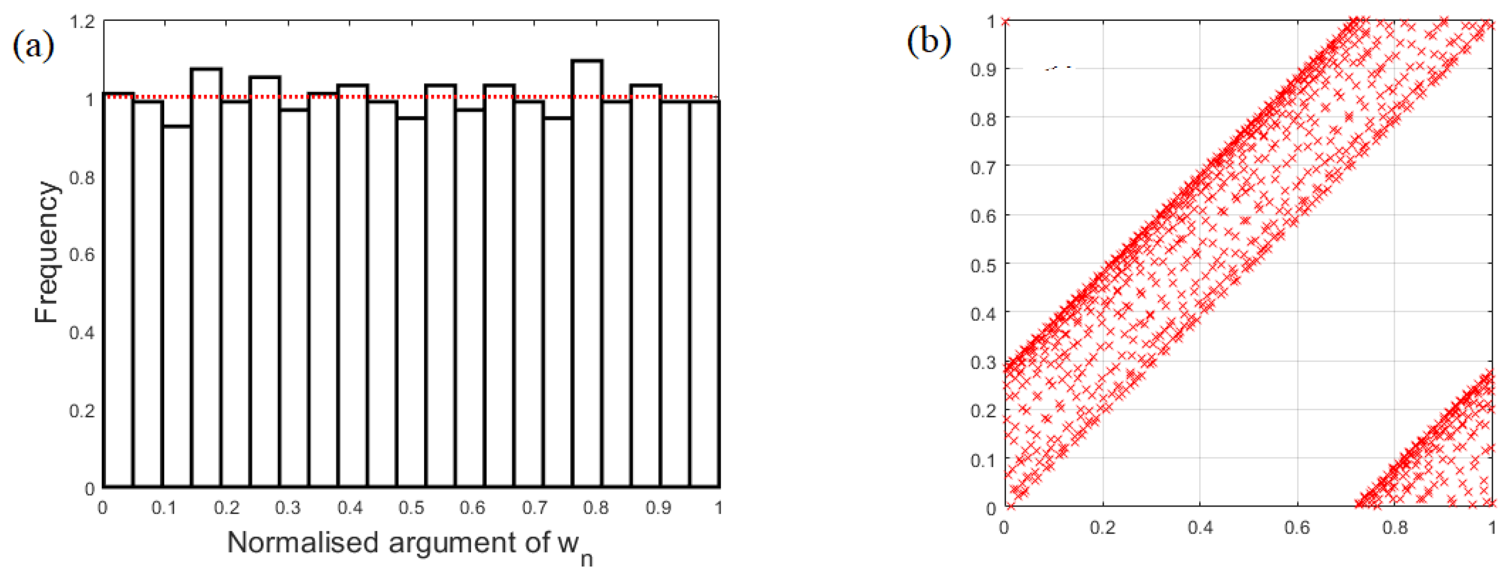
2.4. Complex Arguments of Horadam Sequences

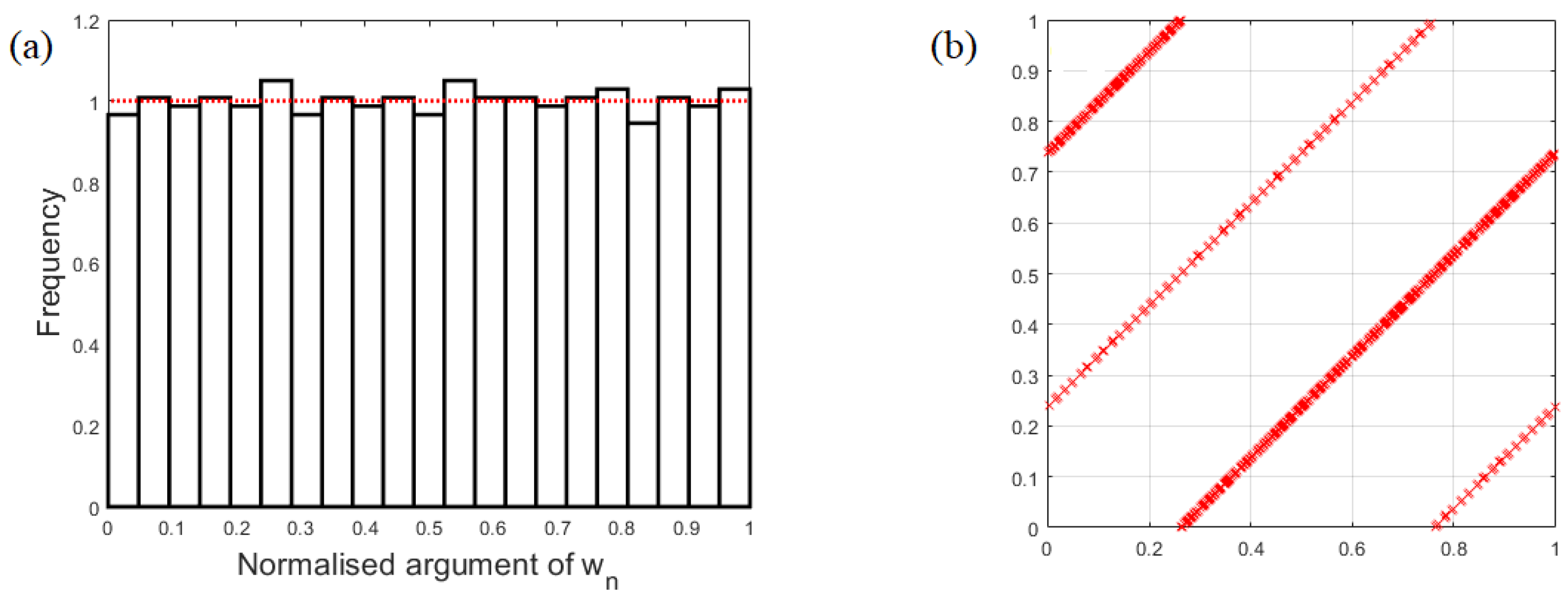
For some dense Horadam sequences, the sequence of complex arguments ${\left({\theta }_n\right)}_{n\ge 0}$ of the Horadam sequence ${\left(w_n\right)}_{n\ge 0}$ in (8) is uniformly distributed in the interval $[-\pi ,\pi ]$. The normalised version of this sequence defined by

$$\begin{array}{c}\hfill {\tilde{\theta }}_n=\frac{{\theta }_n+\pi }{2\pi },n=0,1,\dots ,\end{array}$$

(10)

will be uniformly distributed in the interval $[0,1]$, in this case. This inspires the definition of a PNRG based on dense Horadam sequences.

2.5. Testing Pseudo-Random Number Generators

We will use some tests to evaluate randomness of the PNRG defined by (10).

(1)

Periodicity. Many PNRGs, such as Lagged Fibonacci Sequences, are in fact using periodic sequences with a long period (see, e.g., [27,28]) Since our sequences will actually be non-periodic, this feature does not require testing.

(2)

Autocorrelation. This property is tested by plotting by the sequence ${(x_k,x_{k+1})}_{k\ge 0}$, within the unit square $[0,1]\times [0,1]$. Good PRNGs would provide a good cover.

(3)

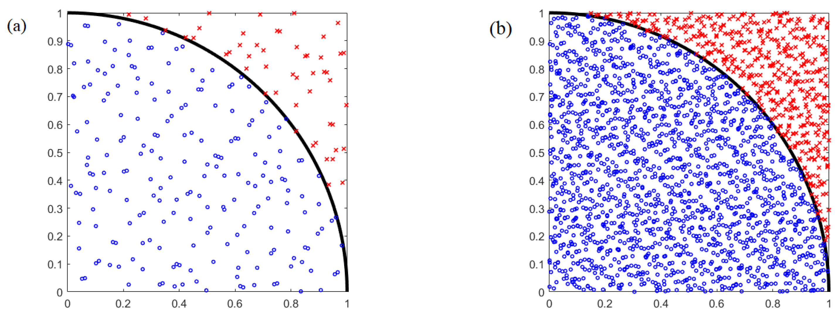
Monte Carlo simulation of $\pi$. For two finite sequences $x_n$, $y_n\in [0,1]$, $n=1,\dots ,N$ given by the algorithm, we count the number $m_N$ of points $(x_n,y_n)$, $n=1,\dots ,N$, falling within the unit circle U, i.e., they satisfy the inequality $x_n^2+y_n^2\le 1$. Based on simple area calculations, the number $\frac{4m_N}{N}$ is used as an approximation for $\pi$.

(4)

NIST tests. These are used to detect the deviations of a binary sequence from randomness. We first generate a finite Horadam sequence ${\left(w_n\right)}_{n=1}^N$, then the normalised complex arguments ${\left(a_n\right)}_{n=1}^N$ (type double) are written as a sequence of binary numbers. We apply the NIST tests which consider the null hypothesis ($H_0$) that the sequence is randomly generated, and the alternative hypothesis ($H_a$). Using the p-value, each test estimates whether the sequence is random (when we say the PNRG passes the test) or non-random. For more technical information one can consult the NIST documentation [31], or the detailed analysis in [32].

3. Testing Complex Arguments of Horadam Sequences: The Case |A| = |B|

In the particular case when $\left|A\right|=\left|B\right|$, the orbit is dense within the disk centred in the origin having radius $2\left|A\right|$, as shown in Figure 1 depicting the sequence obtained for the parameter values $r_1=r_2=1$, $x_1=\frac{\pi }{5}$, $x_2=\frac{e^2}{4}$ and $a=1+\frac{1}{3}i$, $b=1.5a{e}^{\pi (x_1+x_2)}$.

Using the notations (7), When $\left|A\right|=\left|B\right|=R>0$, the relation (8) reduces to

$$\begin{array}{c}\hfill w_n=r_n{e}^{i{\theta }_n}=R\left(e^{i({\varphi }_1+2\pi n{x}_1)}+e^{i({\varphi }_2+2\pi n{x}_2)}\right),\end{array}$$

(11)

hence the sequence of arguments for ${\left(w_n\right)}_{n\ge 0}$ is given by

$$\begin{array}{c}\hfill {\theta }_n=\frac{{\varphi }_1+{\varphi }_2}{2}+2\pi n(x_1+x_2).\end{array}$$

(12)

For 1, $x_1$, $x_2$ linearly independent over $\mathbb{Z}$, the sequence of arguments ${\theta }_n$ is uniformly distributed in the interval $[-\pi ,\pi ]$, and in particular, it is aperiodic.

3.1. Uniform Distribution and Autocorrelation of Arguments

The sequence of normalised arguments ${\tilde{\theta }}_n$ defined by (10) is uniformly distributed in the interval $[0,1]$, as illustrated in Figure 2a. For good PNRGs generators, the 2D diagrams of normalised arguments $({\tilde{\theta }}_n,{\tilde{\theta }}_{n+1})$ would uniformly cover the unit square. However, Figure 2b suggests that consecutive arguments are highly correlated.

3.2. Mixing Arguments and Monte Carlo Based Methods

To address the autocorrelation issue, we approximate $\pi$ using complex arguments of two Horadam sequences ${\left(w_n^1\right)}_{n\ge 0}$ and ${\left(w_n^2\right)}_{n\ge 0}$ for which $\left|A\right|=\left|B\right|$ in Formula (8). The parameters $(x_1,x_2,a,b)$ generating the sequences in (7) are

$$\begin{array}{cc}\hfill & w_n^1:x_1=\frac{e}{2},x_2=\frac{e^2}{4},a=1+\frac{1}{3}i,b=1.5a{e}^{\pi (x_1+x_2)}\hfill \end{array}$$

(13)

$$\begin{array}{cc}\hfill & w_n^2:x_1=\frac{\sqrt{3}}{5},x_2=\frac{\pi }{4},a=1+\frac{2}{3}i,b=1.5a{e}^{\pi (x_1+x_2)},\hfill \end{array}$$

(14)

where the orbit of ${\left(w_n^1\right)}_{n\ge 0}$ was plotted in Figure 1. We denote the normalised arguments ${\left({\theta }_n^1\right)}_{n\ge 0}$, ${\left({\theta }_n^2\right)}_{n\ge 0}$ of sequences ${\left(w_n^1\right)}_{n\ge 0}$, ${\left(w_n^2\right)}_{n\ge 0}$ by $x_n:={\theta }_n^1$, $y_n:={\theta }_n^2$, $n=0,1,\dots$.

We now calculate points $(x_n,y_n)$, $n=1,\dots ,N$ in the unit square $[0,1]\times [0,1]$, and denote by $m\left(N\right)$ how many points fall inside the unit circle, i.e., $x_n^2+y_n^2\le 1$. The formula $4\frac{m\left(N\right)}{N}$ approximates $\pi$, with values expected to improve for larger N. For example, in the simulation shown in Figure 3a, the sample size is $N=1000$ and there are $m_N=794$ points satisfying $x_n^2+y_n^2\le 1$, $n=1,\dots ,N$. One obtains

$$\begin{array}{c}\hfill \frac{m\left(N\right)}{N}=\frac{794}{1000}=0.794\mathrm{and}\pi \sim 4\frac{m\left(N\right)}{N}=3.1760.\end{array}$$

(15)

The value significantly improves with the increase in the number of sequence terms, to $3.1412$ for $N={10}^4$ (depicted in Figure 3b) and to $3.1416$ for $N={10}^6$.

In

Table 1. Absolute errors in the approximation of $\pi$.

10${}^{\mathit{N}}$	MLF	MT	Horadam $\left(\right|\mathit{A}|=|\mathit{B}\left|\right)$	Horadam $\left(\right|\mathit{A}|\ne |\mathit{B}\left|\right)$
1	0.3297	0.7258	0.0584	0.3415
2	0.0615	0.0215	0.0216	0.0184
3	0.0304	0.0456	0.0344	0.0575
4	0.0200	0.0036	0.0004	0.0371
5	0.0018	0.0004	0.0014	0.0523
6	0.0010	0.0026	0.0000	0.0452

, we estimate the error $\left|4\frac{m\left(N\right)}{N}-\pi \right|$, $N={10}^k$, $k=1,\dots ,7$ terms, for points $(x_n,y_n)$, $n=1,\dots ,N$ computed by Multiplicative Lagged Fibonacci with period $2^{32}$ (MTF), Mersenne Twister (MT), and Horadam sequences with $\left|A\right|=\left|B\right|$ and $\left|A\right|\ne \left|B\right|$.

One may notice that the convergence is not monotonic, but the Horadam based PRNG results are comparable, or sometimes exceeds the other simulations, for $\left|A\right|=\left|B\right|$.

A more detailed evaluation of the PNRG in this particular test was provided in [26], where it was tested against approximations of $\pi$ obtained from Multiplicative Lagged Fibonacci and the Mersenne Twister pseudo-random number generators implemented in Matlab (the latter is the default random number generator).

4. Testing Complex Arguments of Horadam Sequences: The Case |A| ≠ |B|

The focus of this section is the case $\left|A\right|\ne \left|B\right|$. By Theorem 4, when the real numbers $1,x_1,x_2$ are linearly independent over $\mathbb{Q}$, the orbit of the Horadam sequence ${\left(w_n\right)}_{n\ge 0}$ given by Formula (8) is dense within the region between two concentric circles centred in the origin, having radii $\left|\right|A|-|B\left|\right|$ and $\left|A\right|+\left|B\right|$. An example is shown in Figure 4, where $r_1=r_2=1,x_1=\frac{\sqrt{2}}{3},x_2=\frac{e}{15}$ and $a=2+\frac{2}{3}i$, $b=3+i$.

As the sequence ${\left(w_n\right)}_{n\ge 0}$ is aperiodic, for the normalised arguments ${\tilde{\theta }}_n$ defined by (10) we will discuss the autocorrelation, approximations of $\pi$, and also the randomness of the sequence ${\tilde{\theta }}_n$ evaluated as a PRNG by the NIST tests.

4.1. Autocorrelation of Arguments

The autocorrelation $({\tilde{\theta }}_n,{\tilde{\theta }}_{n+1})$ for $\left|A\right|\ne \left|B\right|$ is depicted in Figure 5. One can notice that the arguments look uniformly distributed, with better covering than in Figure 2.

4.2. Evaluation of the PNRG by the NIST Tests

To evaluate the suitability of our proposed method as a PRNG, we carried out randomness tests specified by the National Institute of Standards and Technology (NIST) on the sequence of normalised complex arguments ${\tilde{\theta }}_n$ given by (10), for two examples.

These tests were performed on two second order Horadam sequences generated by Formula (1). The proposed PRNG was implemented in C++ on an x64 processor architecture. IEEE 754 Double precision floating point format were used to represent the real and imaginary part of complex numbers. The storage complexity for our PRNG is $O\left(N\right)$, where N denotes the order of the Horadam sequence used by the generator.

The two sequences are generated by the configurations $(x_1,x_2,a,b)$ below:

$$\begin{array}{cc}\hfill & w_n^1:x_1=\frac{\sqrt{2}}{3},x_2=\frac{e}{15},a=2+\frac{2}{3}i,b=3+i\hfill \end{array}$$

(16)

$$\begin{array}{cc}\hfill & w_n^2:x_1=\frac{\sqrt{2}}{3},x_2=\frac{\sqrt{5}}{15},a=2+\frac{2}{3}i,b=3+i.\hfill \end{array}$$

(17)

Calculations use the recurrence Formula (1), where $w_0=a$, $w_1=b$, $p=z_1+z_2$, and $q=-z_1{z}_2$, with $z_1,z_2$ computed from (7). In our implementation, this second order generator used 64 bytes of memory to store two coefficients p and q and two initial seeds $w_0$ and $w_1$. Notice that the sequence ${\left(w_n^1\right)}_{n\ge 0}$ given by (16) was depicted in Figure 4.

For each of these sequences we generate 10,000 terms, converting the floating point values into their corresponding 64-bit binary forms for the randomness tests.

Table 2. NIST randomness tests for sequence ${\left(w_n^1\right)}_{n\ge 0}$ given by (16).

Type of Test	p-Value	Conclusion
01. Frequency Test (Monobit)	0.0	Non-Random
02. Frequency Test within a Block	4.4999 × 10−260	Non-Random
03. Run Test	0.0	Non-Random
04. Longest Run of Ones in a Block	0.0	Non-Random
05. Binary Matrix Rank Test	0.1176	Random
06. Discrete Fourier Transform (Spectral) Test	0.0	Non-Random
07. Non-Overlapping Template Matching Test	6.3061 × 10−5	Non-Random
08. Overlapping Template Matching Test	0.0	Non-Random
09. Maurer’s Universal Statistical test	5.3335 × 10−71	Non-Random
10. Linear Complexity Test	0.3767	Random
11. Serial test (a):	0.0	Non-Random
11. Serial test (b):	0.9972	Random
12. Approximate Entropy Test	0.0	Non-Random
13. Cumulative Sums (Forward) Test	0.0	Non-Random
14. Cumulative Sums (Reverse) Test	0.0	Non-Random

and

Table 3. NIST randomness tests for sequence ${\left(w_n^2\right)}_{n\ge 0}$ given by (17).

Type of Test	p-Value	Conclusion
01. Frequency Test (Monobit)	0.0	Non-Random
02. Frequency Test within a Block	4.5927 × 10−225	Non-Random
03. Run Test	0.0	Non-Random
04. Longest Run of Ones in a Block	0.0	Non-Random
05. Binary Matrix Rank Test	0.4676	Random
06. Discrete Fourier Transform (Spectral) Test	0.0	Non-Random
07. Non-Overlapping Template Matching Test	1.02391 × 10−6	Non-Random
08. Overlapping Template Matching Test	0.0	Non-Random
09. Maurer’s Universal Statistical test	3.3838 × 10−44	Non-Random
10. Linear Complexity Test	0.7255	Random
11. Serial test (a):	0.0	Non-Random
11. Serial test (b):	0.9920	Random
12. Approximate Entropy Test	0.0	Non-Random
13. Cumulative Sums (Forward) Test	0.0	Non-Random
14. Cumulative Sums (Reverse) Test	0.0	Non-Random

indicate that out of the first 14 NIST tests, the proposed PRNG passes

• 05. Binary Matrix Rank Test.
• 10. Linear Complexity Test.
• 11. Serial test (second part).

While these 14 tests agree on these two sequences, it would be expected that the results may slightly differ for other parameter values.

The random excursion tests on both sequences shown promising results as seen in

Table 4. NIST random excursion test for sequence ${\left(w_n^1\right)}_{n\ge 0}$ given by (16).

State	Chi Square	p-Value	Conclusion
−4	4.3483	0.5004	Random
−3	3.0119	0.6982	Random
−2	7.5168	0.1850	Random
−1	10.5714	0.0606	Random
+1	7.1429	0.2102	Random
+2	7.3157	0.1982	Random
+3	5.5607	0.3513	Random
+4	9.4578	0.0921	Random

and

Table 5. NIST random excursion test for sequence ${\left(w_n^2\right)}_{n\ge 0}$ given by (17).

State	Chi Square	p-Value	Conclusion
−4	0.2857	0.9979	Random
−3	0.4	0.9953	Random
−2	6.6667	0.2466	Random
−1	3.0	0.6700	Random
+1	1.0	0.9626	Random
+2	9.3333	0.0965	Random
+3	29.7040	1.6865 × 10−5	Non-Random
+4	5.3953	0.3696	Random

, where apart from ${\left(w_n^2\right)}_{n\ge 0}$ evaluated at state $+3$ which suggested that the sequence was Non-Random, all the other tests concluded that the sequences are Random. We expect that different results may be obtained for other parameter values.

5. The Case of Third-Order Horadam Sequences

We now test the design of a PRNG based on generalized Horadam sequences of third order. Let us first establish some theoretical results. The characteristic equation of the third-order sequence ${\left(w_n\right)}_{n\ge 0}$ described by the relation (4) is the cubic

$$\begin{array}{c}\hfill Q\left(x\right)=x^3-p{x}^2-qx-r=\left(x-z_1\right)\left(x-z_2\right)\left(x-z_3\right),\end{array}$$

whose roots parametrised as $z_1=r_1{e}^{2\pi i{x}_1}$, $z_2=r_2{e}^{2\pi i{x}_2}$, $z_3=r_3{e}^{2\pi i{x}_3}$ will be called generators, linked to the coefficients p, q, and r of the recursion by Vieta’s relations

$$\begin{array}{c}\hfill p=z_1+z_2+z_3,q=-\left(z_1{z}_2+z_2{z}_3+z_1{z}_3\right),r=z_1{z}_2{z}_3,\end{array}$$

(18)

When the generators $z_1$, $z_2$, and $z_3$ are distinct, the general term is given by the formula

$$\begin{array}{c}\hfill w_n=r_n{e}^{i{\theta }_n}=A{z}_1^n+B{z}_2^n+C{z}_3^n,\end{array}$$

(19)

where the constants A, B, and C can be obtained from (19) and the initial conditions

$$\begin{array}{cc}\hfill w_0& =A+B+C=a,\hfill \\ \hfill w_1& =A{z}_1+B{z}_2+C{z}_3=b,\hfill \\ \hfill w_2& =A{z}_1^2+B{z}_2^2+C{z}_3^2=c,\hfill \end{array}$$

where the seeds a, b, and c are given complex numbers. For more details on these calculations and explicit formulae for A, B, and C one can check [24,25].

An atlas of general third-order complex linear recurrences is given in ([22], Chapter 6). Similarly to the classical Horadam sequences the orbits can be dense when the generators are located on the unit circle, i.e., $r_1=r_2=r_3=1$, and when $1,x_1,x_2,x_3$ are linearly independent over $\mathbb{Q}$ (see Proposition 2).

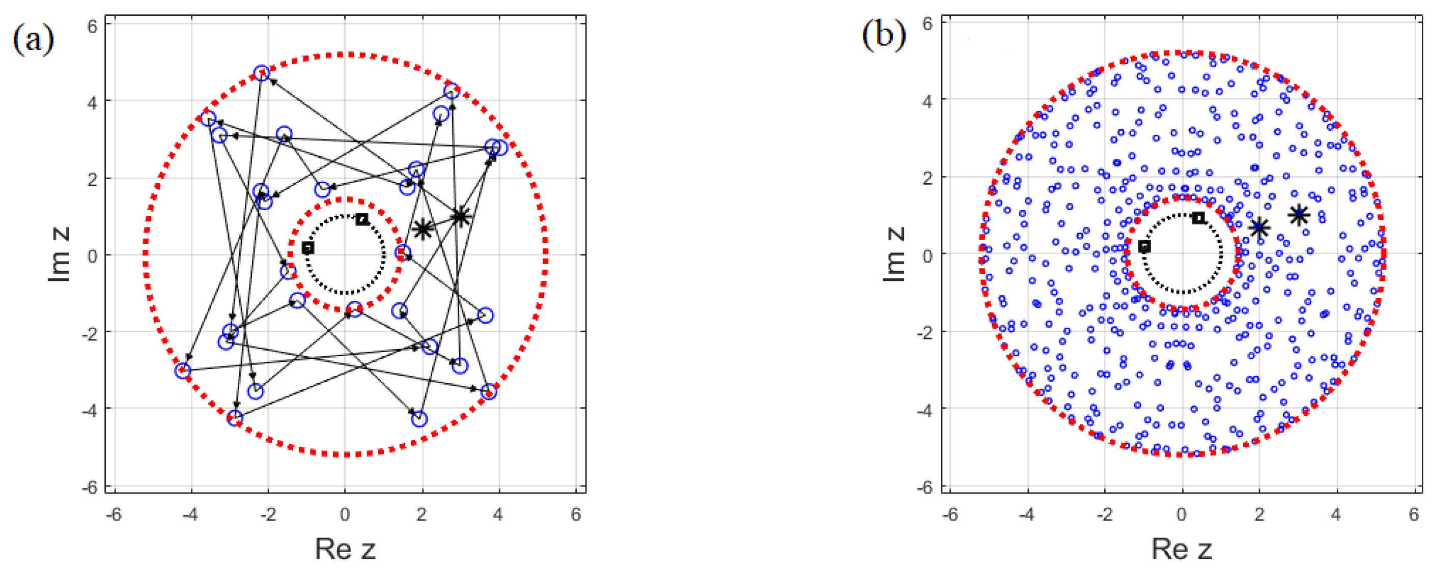
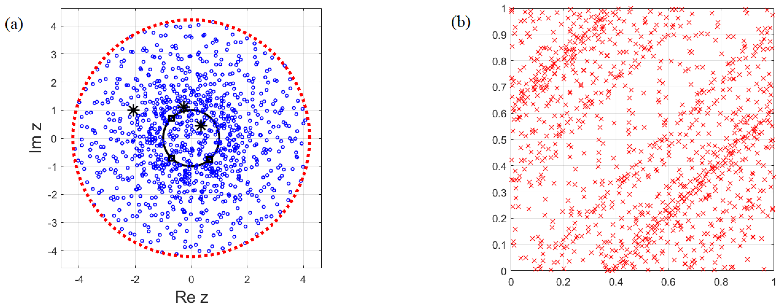
In Figure 6a we illustrate such an example. The sequence ${\left(w_n\right)}_{n\ge 0}$ is computed using the recurrence Formula (4), for the recurrence coefficients p, q, and r given by (18), with generators obtained for $x_1=\frac{\pi }{5}$, $x_2=\sqrt{3}/2$, $x_3=\sqrt{5}/6$ and the seeds $a=0.2e^{2\pi /7+\pi /3}$, $b=0.4e^{6\pi /7+\pi /3}$, and $c=0.8e^{10\pi /7+\pi /3}$. By Formula (19), since $|z_1|=|z_2|=|z_3|=1$, by the triangle inequality one can easily obtain the inequality $|w_n|\le |A|+|B|+|C|$, hence the orbit is located within the circle of radius $\left|A\right|+\left|B\right|+\left|C\right|$, centred in the origin.

5.1. Autocorrelation of Arguments

For the chosen sequence ${\left(w_n\right)}_{n\ge 0}$ displayed in Figure 6a, the sequence ${\left({\theta }_n\right)}_{n\ge 0}$ of complex arguments from Formula (19) is normalised as before through the transformation ${\tilde{\theta }}_n=\frac{{\theta }_n+\pi }{2\pi },n=0,1,\dots$. This sequence also seems to be uniformly distributed.

The autocorrelation obtained for normalised arguments $({\tilde{\theta }}_n,{\tilde{\theta }}_{n+1})$ in Figure 6b indicates that a PNRG based on a third-order Horadam sequence provides a more uniform covering of the unit square $[0,1]\times [0,1]$.

5.2. Evaluation of NIST Tests

As in Section 4.2, we apply the NIST tests on the sequence of normalised complex arguments ${\tilde{\theta }}_n$, computed for the third order Horadam sequence plotted in Figure 6a. The current implementation requires 96 bytes.

Table 6. NIST randomness tests on a third order Horadam sequence.

Type of Test	p-Value	Conclusion
01. Frequency Test (Monobit)	0.0	Non-Random
02. Frequency Test within a Block	8.3042 × 10−249	Non-Random
03. Run Test	0.0	Non-Random
04. Longest Run of Ones in a Block	0.0	Non-Random
05. Binary Matrix Rank Test	0.1839	Random
06. Discrete Fourier Transform (Spectral) Test	0.0	Non-Random
07. Non-Overlapping Template Matching Test	2.8299 × 10−5	Non-Random
08. Overlapping Template Matching Test	0.0	Non-Random
09. Maurer’s Universal Statistical test	3.5207 × 10−76	Non-Random
10. Linear Complexity Test	0.1191	Random
11. Serial test (a):	0.0	Non-Random
11. Serial test (b):	0.0145	Random
12. Approximate Entropy Test	0.0	Non-Random
13. Cumulative Sums (Forward) Test	0.0	Non-Random
14. Cumulative Sums (Reverse) Test	0.0	Non-Random

suggests that from the first 14 NIST tests, the proposed PRNG passes the Binary Matrix Rank (05), the Linear Complexity (10), and the Serial tests (11, part 2). The results are very similar to those for classical Horadam sequences in Table 2 and Table 3.

Table 7. NIST random excursion test on a third order Horadam sequence.

State	Chi Square	p-Value	Conclusion
−4	2.5714	0.7657	Random
−3	3.6000	0.6083	Random
−2	4.5185	0.4774	Random
−1	2.7778	0.7342	Random
+1	3.2222	0.6658	Random
+2	5.8107	0.3251	Random
+3	5.7360	0.3328	Random
+4	13.2979	0.0207	Random

suggests that all random excursion tests conclude that the proposed sequence is Random, similar to the results shown in Table 4. More research is required to establish whether the results hold for other parameter values.

6. Radii of Horadam Sequence Terms

We here investigate the distribution of radii of Horadam sequences. By Formula (7) we have $\left|A\right|=R_1>0$, $\left|B\right|=R_2>0$, while the notations in Formula (8) can by simplified by taking ${\theta }_1={\varphi }_1+n{x}_2,{\theta }_2={\varphi }_2+n{x}_2$, to obtain

$$\begin{array}{c}\hfill r{e}^{i\theta }=R_1{e}^{i{\theta }_1}+R_2{e}^{i{\theta }_2},\end{array}$$

(20)

therefore one has

$$\begin{array}{c}\hfill r^2=R_1^2+R_2^2+2R_1{R}_{2}cos({\theta }_1-{\theta }_2).\end{array}$$

(21)

6.1. The Distribution of Radii for $\left|A\right|=\left|B\right|$

The case $R=R_1=R_2$ is easier to examine. Indeed, the Formula (21) reduces to

$$\begin{array}{c}\hfill r=2Rcos\left(\frac{1}{2}({\theta }_1-{\theta }_2)\right).\end{array}$$

The angle ${\theta }_1-{\theta }_2$ is uniformly distributed in $(-\frac{\pi }{2},\frac{\pi }{2})$, and by denoting $\alpha ={\theta }_1-{\theta }_2$ and $\left|r\right|=2Rcos\left(\alpha \right)$, one may write

$$P\left(\right|r/\left(2R\right)|\ge x)=P(\alpha \le arccos\left(x\right))=\frac{2}{\pi }arccos\left(x\right),$$

for every value x in the interval $(0,1)$. Thus, the density of r is given by the formula

$$\begin{array}{c}\hfill f_r\left(x\right)=\frac{{\mathbf{1}}_{\left|x\right|<2R}}{\pi \sqrt{4R^2-x^2}},\end{array}$$

(22)

where ${\mathbf{1}}_{\left|x\right|<2R}$ represents the indicator function for the disk $U(0;2R)$. The histogram of $|w_n|$ for ${\left(w_n\right)}_{n=0}^{1000}$ is shown in Figure 7a, against the density given by (22). The Horadam sequence used in this case is the one from Section 3, plotted in Figure 1b.

6.2. The Distribution of Radii for $\left|A\right|\ne \left|B\right|$

If $\left|A\right|\ne \left|B\right|$, from the example depicted in Figure 4, the orbits in this case are bounded by two circles. As Figure 7b suggests, these inner and outer bounds are singularities for the radius distribution. We now find the distribution of the radius r, using the notation $r^2=r_1^2+r_2^2+2r_1{r}_{2}cos\left(\alpha \right)$ where $\alpha$ is uniformly distributed in $(0,\pi )$.

As $-1\le ({\theta }_1-{\theta }_2)\le 1$ one has ${(r_1-r_2)}^2\le r^2\le {(r_1+r_2)}^2$, therefore

$$P[r\le x]=\left\{\begin{array}{cc}0\hfill & ,x\le |r_1-r_2|\hfill \\ 1\hfill & ,x\ge r_1+r_2\hfill \end{array}\right..$$

For $|r_1-r_2|<x<r_1+r_2$ we have

$$\begin{array}{cc}\hfill P[r\ge x]& =P[r^2\ge x^2]=P[r_1^2+r_2^2+2r_1{r}_{2}cos\left(\alpha \right)\ge x^2]\hfill \\ \hfill & =P\left[cos\alpha \ge \frac{x^2-r_1^2-r_2^2}{2r_1{r}_2}\right]\hfill \\ \hfill & =P\left[\alpha \le arccos\left(\frac{x^2-r_1^2-r_2^2}{2r_1{r}_2}\right)\right]=\frac{1}{\pi }arccos\left(\frac{x^2-r_1^2-r_2^2}{2r_1{r}_2}\right).\hfill \end{array}$$

By differentiating, one obtains the density function

$$\begin{array}{c}\hfill f_r\left(x\right)=\frac{1}{C}\frac{x}{\sqrt{\left[{(r_1+r_2)}^2-x^2\right]\left[x^2-{(r_1-r_2)}^2\right]}},|r_1-r_2|<x<r_1+r_2.\end{array}$$

(23)

This has singularities at the boundaries $x=|r_1-r_2|$, and $x=r_1+r_2$, and a critical point at $x=\sqrt{|r_1-r_2|\left(r_1+r_2\right)}$. Moreover, we have

$$\begin{array}{c}\hfill f_r^{\prime }\left(x\right)=\frac{1}{C}\frac{x^4-{(r_1-r_2)}^2{(r_1+r_2)}^2}{{\left[{(r_1+r_2)}^2-x^2\right]}^{3/2}{\left[x^2-{(r_1-r_2)}^2\right]}^{3/2}},\end{array}$$

while the constant $C=\pi /2$ ensures that the density $f_r$ given by (23) satisfies

$${\int }_{|r_1-r_2|}^{r_1+r_2}{f}_r\left(x\right)=1.$$

7. Conclusions

We have first discussed the key properties of complex Horadam sequences of second and third order, including exact formulae for the general term. For sequences whose orbits were dense within a 2D region, we analysed the sequence ${\left({\tilde{\theta }}_n\right)}_{n\ge 0}$ of complex arguments normalised to the interval $[0,1]$ by the Formula (10).

In Section 3, we showed that the normalised arguments ${\tilde{\theta }}_n$ are uniformly distributed in the interval $[0,1]$ when A, B given by (3) satisfy $\left|A\right|=\left|B\right|$, which inspired a PNRG. We showed that the autocorrelation of a single sequence was linear, but Monte Carlo simulations for the value of $\pi$ using two distinct sequences showed good convergence properties against established generators (Lagged Fibonacci and Mersenne Twister).

In Section 4 we explored the case $\left|A\right|\ne \left|B\right|$. The autocorrelation was better, but surprisingly, the errors in the approximation of $\pi$ obtained for pairs of Horadam sequences was sometimes worse than for $\left|A\right|=\left|B\right|$, as shown in Table 1. The PRNG generated for two sequences (16) and (17) passed 3 out of 14 NIST tests (8, 10, and 11) (see Table 2 and Table 3). The performance was better in the random excursion tests (see Table 4 and Table 5).

Section 5 presents results for third-order generalized Horadam sequences, where we also explore the properties of a similarly defined PNRG. Results are much improved in terms of autocorrelation, but similar in terms of the NIST tests.

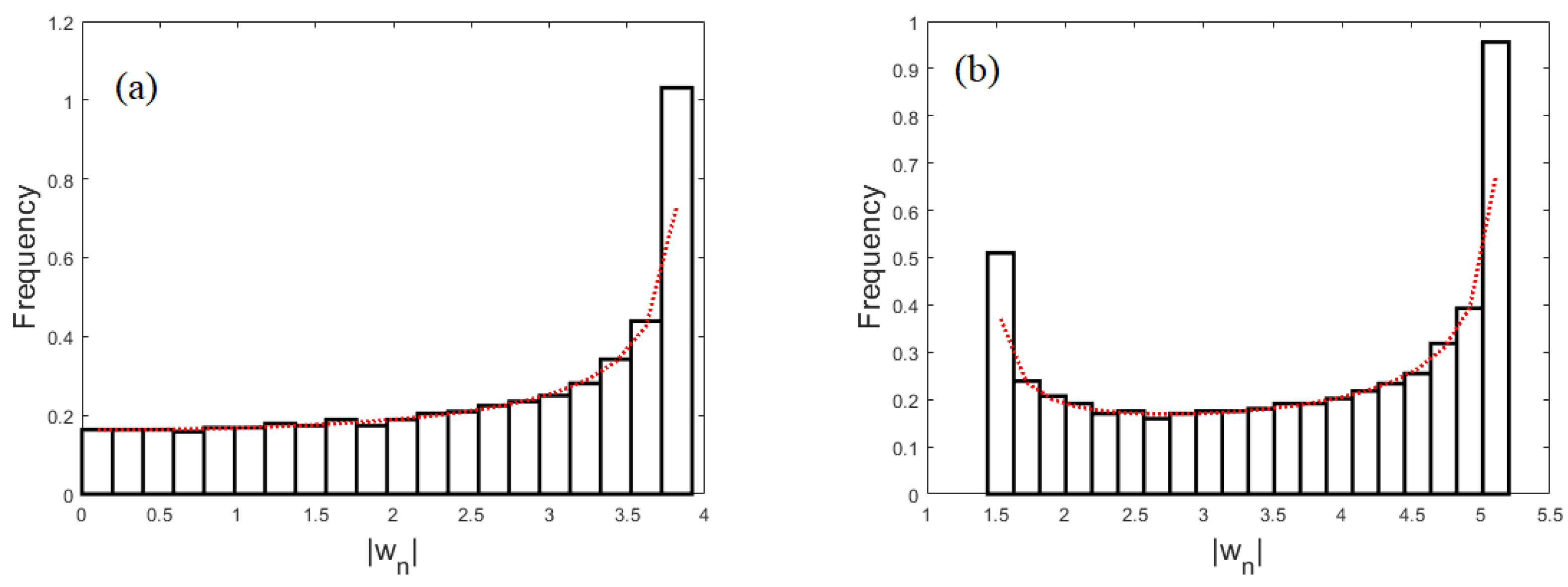
In Section 6 we derived the probability density of the radii of Horadam sequences in the scenarios $\left|A\right|=\left|B\right|$ and $\left|A\right|\ne \left|B\right|$, validated against numerical simulations.

Further investigations are required for understanding the relationship between the initial parameters and the results in the NIST tests, or autocorrelation.