Article

Finite-Time Bounded Tracking Control for a Class of Neutral Systems

1
School of Mathematics and Physics, University of Science and Technology Beijing, No. 30 Xueyuan Road, Haidian District, Beijing 100083, China
2
Institute of Fundamental and Interdisciplinary Sciences, Beijing Union University, No. 97 Beisihuan East Road, Chaoyang District, Beijing 100101, China
3
Institute of Mathematics and Physics, Beijing Union University, No. 97 Beisihuan East Road, Chaoyang District, Beijing 100101, China
4
School of Mathematics and Statistics, Chongqing Technology and Business University, Chongqing 400067, China
5
School of Automation and Electrical Engineering, University of Science and Technology Beijing, No. 30 Xueyuan Road, Haidian District, Beijing 100083, China
6
School of Intelligence Science and Technology, University of Science and Technology Beijing, No. 30 Xueyuan Road, Haidian District, Beijing 100083, China
*
Author to whom correspondence should be addressed.
Mathematics 2023, 11(5), 1199; https://doi.org/10.3390/math11051199
Submission received: 19 January 2023 / Revised: 23 February 2023 / Accepted: 23 February 2023 / Published: 28 February 2023
(This article belongs to the Topic Dynamical Systems: Theory and Applications)

Abstract

:
In this paper, we investigate finite-time bounded (FTB) tracking control for a class of neutral systems. Firstly, the dynamic equation of the tracking error signal is given based on the original neutral system. Then, we combine it with the equations of the state vector to construct an error system, where the reference signal and the disturbance signal are fused in a new vector. Next, about the error system, we study the input–output finite-time stability problem of the closed-loop system by utilizing the Lyapunov–Krasovskii functional. We also give a finite-time stability condition in the form of linear matrix inequalities (LMIs). Furthermore, the delay-dependent and delay-independent finite-time bounded tracking controllers are designed separately for the original system. Finally, a realistic example is given to show the effectiveness of the controller design method in the paper.

1. Introduction

As time tends to infinity, asymptotic stability can guarantee the asymptotic convergence of tracking errors and state trajectories. So it has always been one of the focuses in the control research [1,2]. However, in practice, it is often required that the stability is reached in a desired time interval, not in infinite time. Thus, the research of finite-time stability emerged as the actuality requires. As an important role in the study of the transient behavior of control systems, finite-time stability can help to improve the control precision, achieve better anti-interference and robustness over a time interval [3,4,5]. Therefore, finite-time stability has drawn considerable attention, and many results have been developed during the past decades [6,7,8,9].
Early in 1961, Dorato proposed the short-time stability in the stability analysis of linear time-varying systems [10]. Finite-time stability (FTS) was firstly put forward by Weiss and Infante during the research on the stability of nonlinear systems in 1967 [11]. Moulay et al. [12] inspired FTS by the theory of differential equations for systems with input delay and state delay. Furthermore, they obtained the responding finite-time controllers, respectively, for scalar linear systems and for the chain of integrators with input delay. Artstein’s model reduction was extended to nonlinear feedback for handling input delays [12]. Some new methods and tools are used to analyze FTS. For example, the polynomial Lyapunov functional approach and the sum-of-squares (SOS) theory were used to investigate FTS of continuous-time polynomial fuzzy systems, and all the proposed conditions are given in the form of SOS [13].
With the development of FTS, the finite-time control problem for various systems has also been widely studied [4,14,15,16,17,18]. Fu and Xu proposed a terminal sliding mode disturbance observer to estimate the augmented disturbance. Additionally, they came up with an algorithm to guarantee fast convergence of the tracking error for a class of MIMO nonlinear systems [19]. However, in [17,20], the authors regarded the output as a component of states, which is not common in control systems. Finite-time bounded (FTB) tracking, belonging to finite-time control, was valued in recent years [6,21,22,23]. It was proposed on the basis of input–output FTS by Amato et al. [24]. FTB tracking is such that, given a bound on the initial condition, the output does not exceed a certain threshold during a specified time interval. Amato et al. extended input–output FTS to impulse systems and linear time-varying systems, and they gave sufficient conditions to ensure input–output FTS timewith different types of input [25,26,27,28].
However, there are few research results related to FTB tracking control for neutral-type systems. On one hand, the achievements on FTB tracking control focus on ordinary time-delay systems and fractional-order systems [21,23]. On the other hand, studies of neutral systems concentrate on H control, guaranteed cost control and observer-based control [29,30,31,32,33]. Additionally, although Ref. [34] studied FTB for a class of neutral systems, it only synthesized an observer but not a tracking controller.
In the paper, we investigate FTB tracking control for a class of neutral systems with disturbance. To figure out this problem, the input–output FTS of the error system is studied. Using a Lyapunov–Krasovskii functional, we obtain two FTS criteria and a FTB corollary in terms of LMIs. On the basis of these FTS or FTB conclusions, we design a controller based on time-delay state feedback for the error system. Thus, the delay-dependent and -independent FTB tracking controllers for the original neutral system are given.
The paper is organized as follows. Section 2 is devoted to problem statements and necessary descriptions of definitions, assumptions, and lemmas. The main results for stability analysis and control design are shown in Section 3. In Section 4, we give a simulation example to show that the designed controllers are effective. Finally, the conclusion is obtained in Section 5.

2. Preliminaries

In the sequel, the following notations are used. R n denotes n -dimensional Euclidean space. R n × m is the set of all n × m real matrices. ∗ refers to the symmetric part of a matrix A. A T is the transpose matrix of A. P > 0 represents that P is a positive definite matrix. I denotes an identity matrix with appropriate dimensions.

2.1. Problem Statements

Consider the following neutral system:
x ˙ ( t ) G x ˙ ( t τ ) = A x ( t ) + A 1 x ( t τ ) + B u ( t ) + E w ( t ) , y ( t ) = C x ( t ) , t 0 , x ( t ) = ϕ ( t ) , t [ τ , 0 ] .
where x ( t ) R n , u ( t ) R m , y ( t ) R p and w ( t ) R q are the state, the input, the output, and the disturbance vector, respectively. τ > 0 denotes the constant time delay, which appears in both the state and the derivative terms of (1). A R n × n , A 1 R n × n , C R p × n , G R n × n , B R n × m , and E R n × q are known matrices. The initial condition ϕ ( t ) is a continuous vector-valued initial function of t [ τ , 0 ] . Define the operator D x ( t ) = x ( t ) G x ( t τ ) .
Let y d ( t ) R p be the reference signal. Then the tracking error is defined as
e ( t ) = y ( t ) y d ( t ) .
For t [ τ , 0 ] , we define y d ( t ) = η ( t ) , where η ( t ) is a continuous vector-valued initial function. Then the initial condition of tracking error is e ( t ) = C ϕ ( t ) η ( t ) .
The purpose of this paper is to investigate the finite-time bounded tracking of system (1). Finite-time bounded tracking means that the output y ( t ) is always in some neighborhood of y d ( t ) . It is the promotion of input–output finite-time stability, which is described as follows.
Definition 1 
([24]). System (1) with u ( t ) = 0 is said to be input–output finite-time stable with respect to c 1 , c 2 , Γ , T , where the scalars c 1 > 0 , c 2 > 0 , T > 0 , and Γ > 0 , if under the zero initial condition ϕ ( t ) = 0 , t [ τ , 0 ] , system (1) satisfies
0 T w T ( t ) w ( t ) d t c 1 2 y T ( t ) Γ y ( t ) c 2 2 , t [ 0 , T ] .
Based on Definition 1, the definition of finite-time bounded tracking is shown as follows.
Definition 2 
([23]). Given scalars c 1 > 0 , c 2 > 0 ,   T > 0 , and the weight matrix Γ > 0 , system (1) is said to achieve the finite-time bounded tracking as for y d ( t ) with respect to c 1 , c 2 , Γ , T , if under the zero-initial condition
ϕ ( t ) = 0 , e ( t ) = C ϕ ( t ) η ( t ) = 0 , t [ τ , 0 ] ,
system (1) satisfies
0 T w T ( t ) w ( t ) d t c 1 2 e T ( t ) Γ e ( t ) c 2 2 , t [ 0 , T ] .

2.2. Some Related Assumptions and Lemmas

To acquire the desired controller, the following assumptions and lemmas are employed in the subsequent developments.
Assumption 1. 
λ i ( G ) < 1 ( i = 1 , 2 , , n ) , where λ i ( G ) is the i th eigenvalue of matrix G.
Remark 1. 
When | | G | | < 1 , the nominal system of system (1) is stable, i.e., system (1) with u ( t ) = w ( t ) = 0 converges to zero. We also call the operator D x ( t ) = x ( t ) G x ( t τ ) stable. If λ i ( G ) < 1 ( i = 1 , 2 , , n ) , we can easily obtain that | | G | | < 1 because λ i ( G ) < | | G | | . So λ i ( G ) < 1 can ensure D x ( t ) = x ( t ) G x ( t τ ) is stable [35,36].
Assumption 2. 
The reference signal y d ( t ) satisfies
0 T y ˙ d T ( t ) y ˙ d ( t ) d t c 2 ,
where c is a given positive constant.
Assumption 3. 
The disturbance w ( t ) satisfies
0 T w ˙ T ( t ) w ˙ ( t ) d t d 2 ,
where d is a given positive constant.
Lemma 1 
([37]). Given constant symmetric matrices Ω 1 , Ω 2 and Ω 3 , where Ω 1 = Ω 1 T and Ω 2 = Ω 2 T > 0 , the matrix inequality
Ω 1 + Ω 3 T Ω 2 1 Ω 3 < 0
holds, if and only if
Ω 1 Ω 3 T Ω 3 Ω 2 < 0 ,   or Ω 2 Ω 3 T Ω 3 Ω 1 < 0 .
Lemma 2 
([38]). For any scalar τ > 0 , a positive definite matrix M R n × n and x ( t ) R n , the following inequality holds:
t τ t x ˙ T ( s ) M x ˙ ( s ) d s 1 τ x T ( t ) x T ( t τ ) M M M M x ( t ) x ( t τ ) .

3. Main Results

In this section, we derive sufficient conditions on finite-time bounded tracking of system (1). Firstly, an error system is constructed. Then, the finite-time stability criterion of the error system is proposed.

3.1. Construction of an Error System

According to Equation (2), deriving e ( t ) a e ( t τ ) yields
e ˙ ( t ) a e ˙ ( t τ ) = C x ˙ ( t ) a C x ˙ ( t τ ) y ˙ d ( t ) + a y ˙ d ( t τ ) ,
where a is a constant, and | a | < 1 .
Making the derivative on both sides of system (1), we can obtain
x ¨ ( t ) G x ¨ ( t τ ) = A x ˙ ( t ) + A 1 x ˙ ( t τ ) + B u ˙ ( t ) + E w ˙ ( t ) .
Denote X ( t ) = e ( t ) x ˙ ( t ) . By Equations (1), (3) and (4), it follows that
X ˙ ( t )   G 0 X ˙ ( t τ ) = A 0 X ( t ) + A 01 X ( t τ ) + B 0 u ˙ ( t ) + E 0 w ˙ ( t ) G d [ y ˙ d ( t ) a y ˙ d ( t τ ) ] , e ( t ) = C 0 X ( t ) , X ( t ) = ϕ 0 ( t ) , t [ τ , 0 ] .
where
G 0 = a I 0 0 G , A 0 = 0 C 0 A , B 0 = 0 B ,
A 01 = 0 a C 0 A 1 , E 0 = 0 E , G d = I 0 ,
C 0 = I 0 , ϕ 0 ( t ) = C ϕ ( t ) η ( t ) ϕ ˙ ( t ) .
Based on the construction of G 0 in system (5), the eigenvalues of G 0 are respectively the eigenvalues of G and a. For | a | < 1 and λ i ( G ) < 1 ( i = 1 , 2 , , n ) in Assumption 1, it is easy to obtain that λ j ( G 0 ) < 1 ( j = 1 , 2 , , n + p ) . According to Remark 1, the operator X ˙ ( t ) G 0 X ˙ ( t τ ) is stable.
Letting W ( t ) = y ˙ d ( t ) y ˙ d ( t τ ) w ˙ ( t ) , we can receive the error systems as follows:
X ˙ ( t ) G 0 X ˙ ( t τ ) = A 0 X ( t ) + A 01 X ( t τ ) + B 0 u ˙ ( t ) + G W W ( t ) , e ( t ) = C 0 X ( t ) , X ( t ) = ϕ 0 ( t ) , t [ τ , 0 ] ,
where G W = G d a G d E 0 . Obviously, system (6) has the same form as system (1), and W ( t ) can be regarded as the disturbance. Furthermore, if the closed-loop of system (6) realizes finite-time tracking control with respect to e ( t ) , then the output vector y ( t ) can track y d ( t ) in finite time.
Remark 2. 
It can be found that W ( t ) in system (6) contains the derivatives of the disturbance signal w ˙ ( t ) of system (1), instead of w ( t ) . Since the input–output finite-time stability of system (6) is the object of our discussion, we put constraints on y ˙ d ( t ) and w ˙ ( t ) in Assumptions 2 and 3, rather than on y d ( t ) or w ( t ) as described in Definition 1.

3.2. Finite-Time Bounded Tracking Control of the Error System

Design the delay-dependent feedback controller for system (6) with the form of
u ˙ ( t ) = K 1 X ( t ) + K 2 X ( t τ ) ,
where K 1 and K 2 are the feedback gain matrices with appropriate dimensions. Then the closed-loop of system (6) is
X ˙ ( t ) G 0 X ˙ ( t τ ) = A ^ 0 X ( t ) + A ^ 01 X ( t τ ) + G W W ( t ) , e ( t ) = C 0 X ( t ) , X ( t ) = ϕ 0 ( t ) , t [ τ , 0 ] .
where A ^ 0 = A 0 + B 0 K 1 , A ^ 01 = A 01 + B 0 K 2 .
For system (7), we have the following theorem.
Theorem 1. 
Under Assumptions 2 and 3, for a given scalar γ 0 , if there exist matrices R > 0 , P i > 0 ( i = 1 , 2 , 3 , 4 ) satisfying
A ^ 0 T P 1 + P 1 A 0 ^ γ P 1 + P 3 1 τ P 4 P 1 A ^ 01 + 1 τ P 4 P 1 G W P 1 G 0 τ A ^ 0 T P 4 A ^ 01 T P 1 + 1 τ P 4 1 τ P 4 0 0 τ A ^ 01 T P 4 G W T P 1 0 R 0 τ G W T P 4 G 0 T P 1 0 0 P 2 τ G 0 T P 4 τ P 4 A ^ 0 τ P 4 A ^ 01 τ P 4 G W τ P 4 G 0 τ P 4 < 0
C 0 T Γ C 0 P 1 ,
R c 2 2 c 1 2 exp ( γ T ) I ,
then e T ( t ) Γ e ( t ) c 2 2 ( t [ 0 , T ] ) holds, i.e., system (7) is input–output finite time with respect to c 1 , c 2 , Γ , T , where c 1 2 2 c 2 + d 2 .
Proof. 
For system (7), a Lyapunov–Krasovskii functional candidate is given by
V = V 1 + V 2 + V 3 + V 4 ,
where
V 1 = X T ( t ) P 1 X ( t ) ,
V 2 = t τ t X ˙ T ( s ) P 2 X ˙ ( s ) d s ,
V 3 = t τ t e γ ( t θ ) X T ( θ ) P 3 X ( θ ) d θ ,
V 4 = τ 0 t + θ t X ˙ T ( s ) P 4 X ˙ ( s ) d s d θ
with P i > 0 ( i = 1 , 2 , 3 , 4 ) . Equations (12)–(14) are the common forms of the Lyapynov–Krasovskii functional for time-delay continuous systems, and Equation (15) is designed for neutral systems. Taking the time derivatives of Equations (12)–(15), respectively, along the trajectory of system (7) yields
V ˙ 1 = X ˙ T ( t ) P 1 X ( t ) + X T ( t ) P 1 X ˙ ( t ) = X T ( t ) A ^ 0 T P 1 + P 1 A ^ 0 X ( t ) + X T ( t τ ) A ^ 01 T P 1 X ( t ) + W T ( t ) G W T P 1 X ( t ) +   X ˙ T ( t τ ) G 0 T P 1 X ( t ) + X T ( t ) P 1 A ^ 01 X ( t τ ) + X T ( t ) P 1 G W W ( t ) + X T ( t ) P 1 G 0 X ˙ ( t τ )
V ˙ 2 = X ˙ T ( t ) P 2 X ˙ ( t ) X ˙ T ( t τ ) P 2 X ˙ ( t τ ) ,
V ˙ 3 = γ t τ t e γ ( t s ) X T ( θ ) P 3 X ( θ ) d θ + X T ( t ) P 3 X ( t ) e γ τ X T ( t τ ) P 3 X ( t τ ) γ t τ t e γ ( t s ) X T ( θ ) P 3 X ( θ ) d θ + X T ( t ) P 3 X ( t ) ,
Let F ˙ ( s ) = X ˙ T ( s ) P 4 X ˙ ( s ) , then
V 4 = τ 0 t + θ t F ˙ ( s ) d s d θ = τ 0 F ( t ) F ( t + θ ) d θ = τ F ( t ) τ 0 F ( t + θ ) d θ = τ F ( t ) t τ t F ( l ) d l .
So
V ˙ 4 = τ F ˙ ( t ) F ( t ) F ( t τ ) = τ F ˙ ( t ) t τ t F ˙ ( s ) d s = τ F ˙ ( t ) t τ t X ˙ T ( s ) P 4 X ˙ ( s ) d s .
Denote ξ = X ( t ) X ( t τ ) W t X ˙ ( t τ ) .
Based on Equations (16), (17) and (19), and inequality (18), we can obtain
V ˙ X T ( t ) A ^ 0 T P 1 + P 1 A ^ 0 + P 3 X ( t ) + X T ( t ) P 1 A ^ 01 X ( t τ ) + X T ( t ) P 1 G W W ( t ) +   X T ( t ) P 1 G 0 X ˙ ( t τ ) + X T ( t τ ) A ^ 01 T P X ( t ) + W T ( t ) G W T P 1 X ( t ) + X ˙ T ( t τ ) G 0 T P 1 X ( t )   X ˙ T ( t τ ) P 2 X ˙ ( t τ ) + γ t τ t e γ ( t s ) X T ( θ ) P 3 X ( θ ) d θ +   τ ξ T ( t ) A ^ 0 A ^ 01 G W G 0 T P 4 A ^ 0 A ^ 01 G W G 0 ξ ( t ) t τ t X ˙ T ( s ) P 4 X ˙ ( s ) d s
According to Lemma 2, we have
t τ t X ˙ T ( s ) P 4 X ˙ ( s ) d s 1 τ X T ( t ) X T ( t τ ) T P 4 P 4 P 4 P 4 X ( t ) X ( t τ ) = 1 τ ξ T t P 4 P 4 0 0 P 4 P 4 0 0 0 0 0 0 0 0 0 0 ξ t .
Combining inequality (21) with inequality (20), we have
V ˙ ξ T t Ω 1 ξ ( t ) + τ ξ T t A ^ 0 T A ^ 01 T G W T G 0 T P 4 A ^ 0 A ^ 01 G W G 0 ξ t + γ t τ t e γ t s X T θ P 3 X θ d θ ,
where
Ω 1 = A ^ 0 T P 1 + P 1 A ^ 0 + P 3 1 τ P 4 P 1 A ^ 01 + 1 τ P 4 P 1 G W P 1 G 0 1 τ P 4 0 0 0 0 P 2 .
Next, we utilize inequalities (8), (9), (10) and (22) to study the FTS for system (7).
In view of τ P 4 < 0 , according to Lemma 1, inequality (8) equals to
Ω 2 τ A ^ 0 T P 4 A ^ 01 T P 4 G W T P 4 G 0 T P 4 τ P 4 1 τ P 4 A ^ 0 τ P 4 A ^ 01 τ P 4 G W τ P 4 G 0 < 0 ,
where
Ω 2 = A ^ 0 T P 1 + P 1 A ^ 0 γ P 1 + P 3 1 τ P 4 P 1 A ^ 01 + 1 τ P 4 P 1 G W P 1 G 0 1 τ P 4 0 0 R 0 P 2 .
Based on the expression of Ω 1 in Equation (23), inequality (24) can be further transformed into the following forms:
Ω 1 + τ A ^ 0 T A ^ 01 T G W T G 0 T P 4 A ^ 0 A ^ 01 G W G 0 + γ P 1 0 0 0 0 0 0 0 0 0 R 0 0 0 0 0 < 0 .
By inequalities (22) and (25), it follows that
V ˙ ξ T ( t ) γ P 1 0 0 0 0 0 0 0 0 0 R 0 0 0 0 0 ξ ( t ) + γ t τ t e γ ( t s ) X T ( θ ) P 3 X ( θ ) d θ = γ X T ( t ) P 1 X ( t ) + W T ( t ) R W ( t ) + γ t τ t e γ ( t s ) X T ( θ ) P 3 X ( θ ) d θ = γ V 1 + γ V 3 + W T ( t ) R W ( t ) γ V + W T ( t ) R W ( t ) ,
so we have
V ˙ ( t ) γ V ( t ) W T ( t ) R W ( t ) .
The following inequality is established:
exp ( γ t ) V ˙ ( t ) γ exp ( γ t ) V ( t ) exp ( γ t ) W T ( t ) R W ( t ) .
Noticing that d d t ( exp ( γ t ) V ( t ) ) = exp ( γ t ) V ˙ ( t ) γ exp ( γ t ) V ( t ) , we obtain
d d t ( exp ( γ t ) V ( t ) ) exp ( γ t ) W T ( t ) R W ( t ) ,
Based on the zero-initial condition in Definition 2, from inequality (27), it can be obtained that
exp γ t V ( t ) 0 t exp ( γ s ) W T ( s ) R W ( s ) d s .
Thus,
V ( t ) exp ( γ t ) 0 t exp ( γ s ) W T ( s ) R W ( s ) d s exp ( γ t ) λ max ( R ) 0 t W T ( s ) W ( s ) d s exp ( γ T ) λ max ( R ) 0 T W T ( s ) W ( s ) d s .
Since e ( t ) = C 0 X ( t ) , based on inequality (9), Equations (11) and (12), we obtain
e T ( t ) Γ e ( t ) = X T ( t ) C 0 T Γ C 0 X ( t ) X T ( t ) P 1 X ( t ) V ( t ) .
In combination with inequalities (28) and (29), it follows that
e T ( t ) Γ e ( t ) exp γ T λ max ( R ) 0 T W T ( t ) W ( t ) d t .
In view of W ( t ) = y ˙ d ( t ) y ˙ d ( t τ ) w ˙ ( t ) , we have
0 T W T ( t ) W ( t ) d t = 0 T y ˙ d T ( t ) y ˙ d T ( t τ ) w ˙ T ( t ) y ˙ d ( t ) y ˙ d ( t τ ) w ˙ ( t ) d t = 0 T y ˙ d T ( t ) y ˙ d ( t ) d t + 0 T y ˙ d T ( t τ ) y ˙ d ( t τ ) d t + 0 T w ˙ T ( t ) w ˙ ( t ) d t .
Then substituting Equation (31) into Equation (30), according to inequality (10), Assumptions 2 and 3, we can obtain
e T ( t ) Γ e ( t ) e γ T λ m a x ( R ) ( 2 c 2 + d 2 ) e γ T λ m a x ( R ) c 1 2 e γ T c 2 2 e γ T c 1 2 c 1 2 c 2 2 .
This proves Theorem 1. □
Furthermore, we give the feedback gain matrices K 1 and K 2 in system (7).
Theorem 2. 
Under Assumptions 2 and 3, for a given scalar γ 0 , if there exist M 1 , M 2 , Z i ( i = 1 , 2 , 3 , 4 ) with appropriate dimensions satisfying
Φ 1 A 01 Z 1 + B 0 M 2 + 1 τ Z 4 G W G 0 Z 1 τ A 0 Z 1 + B 0 M 1 T 1 τ Z 4 0 0 τ A 01 Z 1 + B 0 M 2 T R 0 τ G W T Z 2 τ Z 1 G 0 T τ Z 4 2 Z 1 < 0
Z 1 Z 1 C 0 T Γ 1 < 0 ,
R c 2 2 e γ T c 1 2 I ,
where Φ 1 = A 0 Z 1 + B 0 M 1 T + A 0 Z 1 + B 0 M 1 γ Z 1 + Z 3 1 τ Z 4 , c 1 2 2 c 2 + d 2 . Then system (7) is input–output finite-time stable with respect to c 1 , c 2 , Γ , T , when K 1 = M 1 Z 1 1 , K 2 = M 2 Z 1 1 .
Proof. 
Multiplying Λ = d i a g ( P 1 1 , P 1 1 , I , P 1 1 , P 4 1 ) by the right and left on both sides of inequality (8) yields
Φ ^ 0 A ^ 01 P 1 1 + 1 τ P 1 1 P 4 P 1 1 G W G 0 P 1 1 τ P 1 1 A ^ 0 T 1 τ P 1 1 P 4 P 1 1 0 0 τ P 1 1 A ^ 01 T R 0 τ G W T P 1 1 P 2 P 1 1 τ P 1 1 G 0 T τ P 4 1 < 0
where Φ ^ 0 = P 1 1 A ^ 0 T + A ^ 0 P 1 1 γ P 1 1 + P 1 1 P 3 P 1 1 1 τ P 1 1 P 4 P 1 1 . Substituting A ^ 0 = A 0 + B 0 K 1 and A ^ 01 = A 01 + B 0 K 2 into inequality (35), we obtain
Φ 0 A 01 P 1 1 + B 0 K 2 P 1 1 + 1 τ P 1 1 P 4 P 1 1 G W G 0 P 1 1 τ P 1 1 A 0 + B 0 K 1 T 1 τ P 1 1 P 4 P 1 1 0 0 τ P 1 1 A 01 + B 0 K 2 T R 0 τ G W T P 1 1 P 2 P 1 1 τ P 1 1 G 0 T τ P 4 1 < 0
where
Φ 0 = ( A 0 P 1 1 + B 0 K 1 P 1 1 ) T + ( A 0 P 1 1 + B 0 K 1 P 1 1 ) γ P 1 1 + P 1 1 P 3 P 1 1 1 τ P 1 1 P 4 P 1 1 .
Denote Z 1 = P 1 1 , M 1 = K 1 P 1 1 , M 2 = K 2 P 1 1 , Z 2 = P 1 1 P 2 P 1 1 , Z 3 = P 1 1 P 3 P 1 1 and Z 4 = P 1 1 P 4 P 1 1 , it can be obtained that inequality (36) equals to the following inequality:
Φ 1 A 01 Z 1 + B 0 M 2 + 1 τ Z 4 G W G 0 Z 1 τ A 0 Z 1 + B 0 M 1 T 1 τ Z 4 0 0 τ A 01 Z 1 + B 0 M 2 T R 0 τ G W T Z 2 τ Z 1 G 0 T τ P 4 1 < 0
where
Φ 1 = A 0 Z 1 + B 0 M 1 T + A 0 Z 1 + B 0 M 1 γ Z 1 + Z 3 1 τ Z 4 .
Obviously, inequality (37) is not an LMI because of the last matrix block τ P 4 1 . To solve inequality (37) by LMI toolbox of MATLAB, we notice that
P 4 1 Z 1 T P 4 P 4 1 Z 1 = P 4 1 2 Z 1 + Z 1 T P 4 1 Z 1 = P 4 1 2 Z 1 + Z 4 .
Because the congruent transformation does not change the positive definiteness of the matrix, the following inequality holds:
P 4 1 Z 1 T P 4 P 4 1 Z 1 0
From Equation (38) and inequality (39), we obtain P 4 1 2 Z 1 + Z 4 0 , i.e.,
P 4 1 Z 4 2 Z 1 .
Therefore, if
Φ 1 A 01 Z 1 + B 0 M 2 + 1 τ Z 4 G W G 0 Z 1 τ A 0 Z 1 + B 0 M 1 T 1 τ Z 4 0 0 τ A 01 Z 1 + B 0 M 2 T R 0 τ G W T Z 2 τ Z 1 G 0 T τ Z 4 2 Z 1 < 0 ,
then inequality (37) holds.
Based on inequality (9), we can derive
Z 1 C 0 T Γ C 0 Z 1 Z 1 0 ,
i.e.,
Z 1 Z 1 C 0 T ( Γ 1 ) 1 C 0 Z 1 0 .
Then according to Lemma 1 and inequality (40), we can acquire
Z 1 Z 1 C 0 T Γ 1 < 0 .
Consequently, if inequalities (32) to (34) hold, then inequalities (8) to (10) are satisfied, i.e., Theorem 1 is true. This proves Theorem 2. □
Denote K 1 = K 1 e K 1 x and K 2 = K 2 e K 2 x . As X ( t ) = e ( t ) x ˙ ( t ) , it follows that
u ˙ ( t ) = K 1 e e ( t ) + K 1 x x ˙ ( t ) + K 2 e e ( t τ ) + K 2 x x ˙ ( t τ ) .
Integrating Equation (41) on interval [ 0 , t ] , we have
u ( t ) = K 1 e 0 t e ( θ ) d θ + K 1 x x ( t ) K 1 x x ( 0 ) + K 2 e τ t τ e ( θ ) d θ + K 2 x x ( t τ ) K 2 x x ( τ ) .
u ( t ) is the delay-dependent finite-time bounded tracking controller of system (1). If we want to design a delay-independent controller, we can take K 2 = 0 , namely, take M 2 = 0 in inequality (32). Thus, the following corollary is received.
Corollary 1. 
Under Assumptions 2 and 3, for a given scalar γ 0 , if there exist M ,   Z i ( i = 1 , 2 , 3 , 4 ) satisfying
Φ 1 A 01 Z 1 + 1 τ Z 4 G W G 0 Z 1 τ A 0 Z 1 + B 0 M T 1 τ Z 4 0 0 τ Z 1 T A 01 T R 0 τ G W T Z 2 τ Z 1 G 0 T τ Z 4 2 Z 1 < 0
Z 1 Z 1 C 0 T Γ 1 < 0 ,
R c 2 2 e γ T c 1 2 I ,
where Φ 1 = A 0 Z 1 + B 0 M T + A 0 Z 1 + B 0 M γ Z 1 + Z 3 1 τ Z 4 , c 1 2 2 c 2 + d 2 , then the output of system (1) realizes the finite-time bounded tracking to the reference signal y d ( t ) under the controller
u t = K e 0 t e θ d θ + K x x t K x x 0 ,
where K e K x = M Z 1 1 .

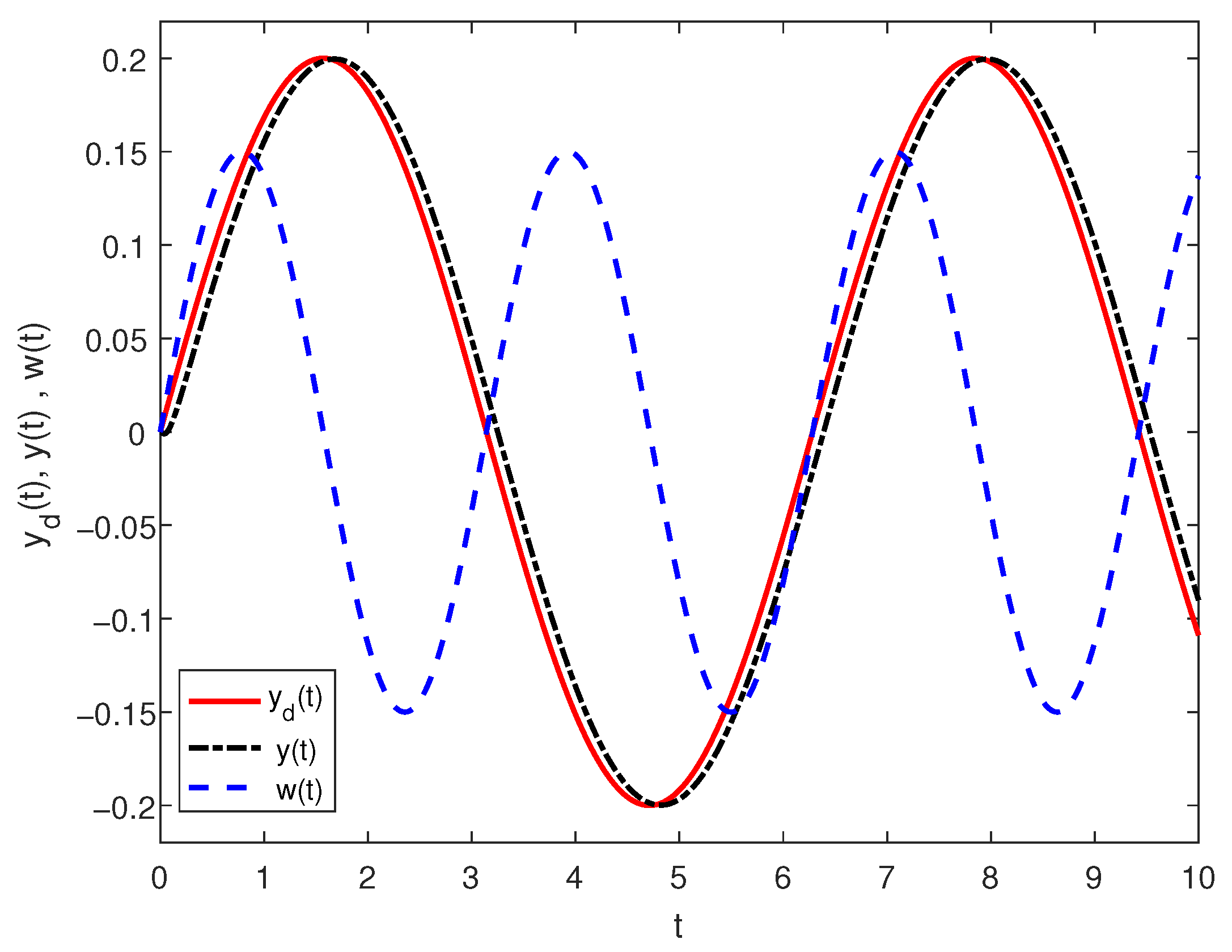
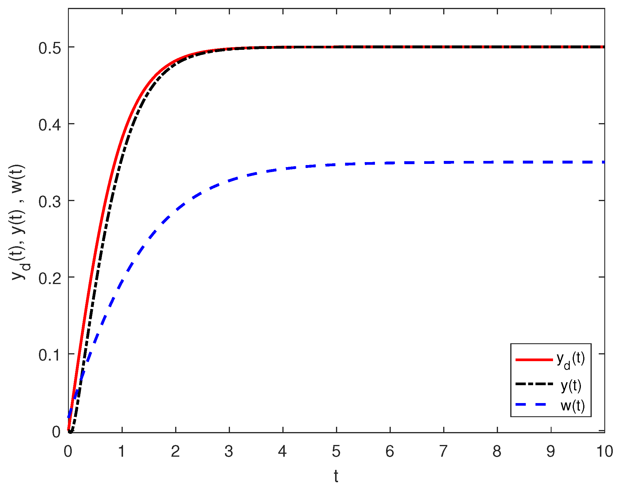
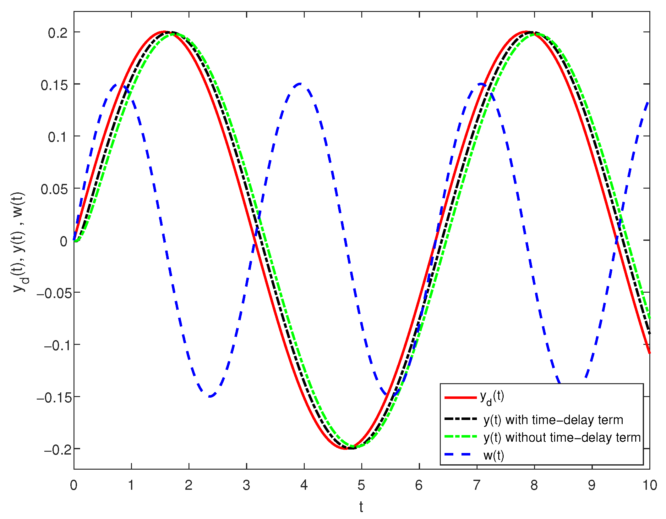
4. Numerical Simulation

In this section, we conduct a realistic delay differential equation of neutral type (NDDE) problem originated from [39] to validate the effectiveness of the results in Section 3.
Example. Figure 1a represents a small metal strip with two cells, and Figure 1b is the partial element equivalent circuits (PEEC) model of the metal strip, which includes the partial inductances L p i j and the partial coefficients of potential p i j . The state vector and the input represent the partial inductance branch currents and the unknown nodal voltages, respectively.
In the model, the coefficient matrices are
A 100 = 7 1 2 3 9 0 1 2 6 , B = 0 1 3 ,
A 1 100 = 1 0 3 0.5 0.5 1 0.5 1.5 0 , E = 0.05 0 0 1 ,
G = 1 72 1 5 2 4 0 3 2 4 1 , C 100 = 1 1 0 ,
and ϕ ( t ) = 0 , for all t [ τ , 0 ] .
Choose the parameters Γ = I , c 1 = 1 , c 2 = 2 , T = 10 and γ = 0.2 . By using LMI toolbox in MATLAB, we conclude that there exists a feasible solution of inequalities (32) to (34) when the time-delay upper bound is 0.003. At this time, the feedback gain matrices are
K 1 = K 1 e K 1 x = 63.3591 0.6543 102.1523 60.3751 ,
K 2 = K 2 e K 2 x = 0.3725 0.4602 41.2559 70.8512 .
Case 1. When
y d ( t ) = 0.2 sin t , t [ 0 , T ] , 0 , t [ τ , 0 ] ,
and
w ( t ) = 0.15 sin ( 2 t ) ,
we have
0 T y ˙ d T ( t ) y ˙ d ( t ) d t 0.25 = def c 2
and
0 T w ˙ T ( t ) w ˙ ( t ) d t 0.5 = def d 2 .
Thus, 2 c 2 + d 2 c 1 2 , and Theorem 2 is satisfied. If we take η ( t ) = 0 , t [ τ , 0 ] , then e ( t ) = C ϕ ( t ) η ( t ) = 0 , t [ τ , 0 ] , and
e T ( t ) Γ e ( t ) c 2 2 ( t [ τ , 0 ] )
holds. The output response is shown in Figure 2.
Case 2. When taking
y d ( t ) = 1 1 + e 2 t 0.5 , t [ 0 , T ] , 0 , t [ τ , 0 ] ,
and
w ( t ) = 2 2 + e t 0.65 ,
one can obtain
0 T y ˙ d T ( t ) y ˙ d ( t ) d t 0.2 = def c 2
and
0 T w ˙ T ( t ) w ˙ ( t ) d t 0.1 = def d 2 .
As a result, 2 c 2 + d 2 c 1 2 , and Theorem 2 holds. The output response is shown in Figure 3.
Figure 2 and Figure 3 indicate that during time period [ 0 , T ] , by the controller (42), the output y ( t ) stays in the c 2 neighborhood of y d ( t ) , i.e., the output of (1) achieves bounded time tracking to the reference signal y d ( t ) .
Case 3. For the disturbance signal and the reference signal in case 1, if we take Equation (46) as the controller, another output response is obtained. The feedback gain matrices are
K 1 = K 1 e K 1 x = 47.7525 36.6115 119.4409 107.9395 .
Putting the output responses in case 1 and the new one together, we can obtain Figure 4.
Figure 4 shows that the tracking effect by using Equation (42) is better than Equation (46). That means the time-delay feedback term is helpful in the tracking problem of neutral systems.

5. Conclusions

In this work, we study FTB tracking control for a class of neutral systems. In order to realize these objectives, we construct an error system for the original neutral systems. Thus, FTB tracking of the original system is transferred to input–output FTS of the error system. For the closed-loop system of error system, we employ the Lyapunov–Krasovskii functional, which contains not only the time-delay term but also the exponential term. The sufficient conditions for the stability of the system are obtained in terms of LMIs. We further derive the finite-time bounded controllers that are delay dependent and delay independent. For further research, the finite-time bounded control problem will be extended to more types of control systems.

Author Contributions

Methodology, Writing-original draft, Y.X.; Methodology, Software, Writing—review and editing, J.W.; Writing—review and editing, H.X.; Formal analysis, Y.Z. All authors have read and agreed to the published version of the manuscript.

Funding

This work was supported in part by Premium Funding Project for Academic Human Resources Development in Beijing Union University under Grant BPHR2020CZ06, and in part by Interdisciplinary Research Project for Young Teachers of University of Science and Technology Beijing (Fundamental Research Funds for the Central Universities) under Grant FRF-IDRY-20-027.

Data Availability Statement

Not applicable.

Conflicts of Interest

The authors declare no conflict of interest.

References

  1. Clarke, F.H.; Ledyaev, Y.S.; Stern, R.J. Asymptotic stability and smooth Lyapunov functions. J. Differ. Equ. 1998, 149, 69–114. [Google Scholar] [CrossRef]
  2. Clarke, F.H.; Ledyaev, Y.S.; Sontag, E.D.; Subbotin, A.I. Asymptotic controllability implies feedback stabilization. IEEE Trans. Autom. Control 1997, 42, 1394–1407. [Google Scholar] [CrossRef]
  3. Bhat, S.P.; Bernstein, D.S. Finite-time stability of continuous autonomous systems. SIAM J. Control Optim. 2000, 38, 751–766. [Google Scholar] [CrossRef]
  4. Amato, F.; Ariola, M.; Cosentino, C. Finite-time stability of linear time-varying systems: Analysis and controller design. IEEE Trans. Autom. Control 2010, 55, 1003–1008. [Google Scholar] [CrossRef]
  5. Lee, J.; Haddad, W.M. On finite-time stability and stabilization of nonlinear hybrid dynamical systems. AIMS Math. 2021, 6, 5535–5562. [Google Scholar] [CrossRef]
  6. Kussaba, H.T.; Borges, R.A.; Ishihara, J.Y. A new condition for finite time boundedness analysis. J. Frankl. Inst. 2015, 352, 5514–5528. [Google Scholar] [CrossRef]
  7. Khoo, S.; Yin, J.; Man, Z.; Yu, X. Finite-time stabilization of stochastic nonlinear systems in strict-feedback form. Automatica 2013, 49, 1403–1410. [Google Scholar] [CrossRef]
  8. Hei, X.; Wu, R. Finite-time stability of impulsive fractional-order systems with time-delay. Appl. Math. Model. 2016, 40, 4285–4290. [Google Scholar] [CrossRef]
  9. Wu, G.C.; Baleanu, D.; Zeng, S.D. Finite–time stability of discrete fractional delay systems: Gronwall inequality and stability criterion. Commun. Nonlinear Sci. 2018, 57, 299–308. [Google Scholar] [CrossRef]
  10. Dorato, P. Short-Time Stability in Linear Time-Varying Systems; Polytechnic Institute of Brooklyn: Ann Arbor, MI, USA, 1961. [Google Scholar]
  11. Weiss, L.; Infante, E.F. Finite time stability under perturbing forces and on product spaces. IEEE Trans. Autom. Control 1967, 12, 54–59. [Google Scholar] [CrossRef]
  12. Moulay, E.; Dambrine, M.; Yeganefar, N.; Perruquetti, W. Finite-time stability and stabilization of time-delay systems. Syst. Control Lett. 2008, 57, 561–566. [Google Scholar] [CrossRef]
  13. Chen, X.; Hu, M. Finite-time stability and controller design of continuous-Time polynomial fuzzy systems. Abstr. Appl. Anal. 2017, 2017, 3273480. [Google Scholar] [CrossRef]
  14. Zimenko, K.; Efimov, D.; Polyakov, A. Adaptive finite-time and fixed-time control design using output stability conditions. Int. J. Robust Nonlinear Control 2022, 32, 6361–6378. [Google Scholar] [CrossRef]
  15. Xu, J.; Wang, L.; Liu, Y.; Sun, J.; Pan, Y. Finite-time adaptive optimal consensus control for multi-agent systems subject to time-varying output constraints. Appl. Math. Comput. 2022, 427, 127176. [Google Scholar] [CrossRef]
  16. Jin, X. Adaptive finite-time tracking control for joint position constrained robot manipulators with actuator faults. In Proceedings of the 2016 American Control Conference (ACC), Boston, MA, USA, 6–8 July 2016; pp. 6018–6023. [Google Scholar]
  17. Zhang, J.; Xia, J.; Sun, W.; Zhuang, G.; Wang, Z. Finite-time tracking control for stochastic nonlinear systems with full state constraints. Appl. Math. Comput. 2018, 338, 207–220. [Google Scholar] [CrossRef]
  18. Jing, Y.; Liu, Y.; Zhou, S. Prescribed performance finite-time tracking control for uncertain nonlinear systems. J. Syst. Sci. Complex. 2019, 32, 803–817. [Google Scholar] [CrossRef]
  19. Fu, M.; Xu, Y. Finite-time tracking control for a class of MIMO nonlinear systems with unknown asymmetric saturations. Math. Probl. Eng. 2017, 2017, 9452171. [Google Scholar]
  20. Huang, S.; Xiang, Z. Finite-time output tracking for a class of switched nonlinear systems. Int. J. Robust Nonlinear Control 2017, 27, 1017–1038. [Google Scholar] [CrossRef]
  21. Xie, H.; Liao, F.; Chen, Y.; Zhang, X.; Li, M.; Deng, J. Finite-time bounded tracking control for fractional-order systems. IEEE Access 2021, 9, 11014–11023. [Google Scholar] [CrossRef]
  22. Gui, H.; Vukovich, G. Finite-time angular velocity observers for rigid-body attitude tracking with bounded inputs. Int. J. Robust Nonlinear Control 2017, 27, 15–38. [Google Scholar] [CrossRef]
  23. Liao, F.; Wu, Y. Finite-time bounded tracking control for linear continuous systems with time-delay. J. Control Decis. 2019, 34, 2095–2104. [Google Scholar]
  24. Amato, F.; Ambrosino, R.; Cosentino, C.; Tommasi, G. Technical communique input-output finite time stabilization of linear systems. J. Control Decis. 2019, 34, 2095–2104. [Google Scholar]
  25. Amato, F.; Carannante, G.; Tommasi, G.D. Input–output finite-time stabilisation of a class of hybrid systems via static output feedback. Int. J. Control 2011, 84, 1055–1066. [Google Scholar] [CrossRef]
  26. Amato, F.; Tommasi, G.D.P.A. Necessary and sufficient conditions for input-output finite-time stability of impulsive dynamical systems. In Proceedings of the 2015 American Control Conference (ACC), Chicago, IL, USA, 1–3 July 2015; pp. 5998–6003. [Google Scholar]
  27. Amato, F.; Tommasi, G.D.; Pironti, A. Input–output finite-time stabilization of impulsive linear systems: Necessary and sufficient conditions. Nonlinear Anal. Hybrid Syst. 2016, 19, 93–106. [Google Scholar] [CrossRef]
  28. Amato, F.; Carannante, G.; Tommasi, G.D.; Pironti, A. Input-output finite-time stabilisation of linear systems with input constraints. IET Control Theory Appl. 2014, 8, 1429–1438. [Google Scholar] [CrossRef]
  29. Haotian, W.; Yanqian, W.; Guangming, Z. Asynchronous H controller design for neutral singular Markov jump systems under dynamic event-triggered schemes. J. Frankl. Inst. Eng. Appl. Math. 2021, 358, 494–515. [Google Scholar]
  30. Aghayan, Z.S.; Alfi, A.; Mousavi, Y.; Kucukdemiral, I.B.; Fekih, A. Guaranteed cost robust output feedback control design for fractional-order uncertain neutral delay systems. Chaos Solitons Fractals 2022, 163, 112523. [Google Scholar] [CrossRef]
  31. Aghayan, Z.S.; Alfi, A.; Machado, J.T. Guaranteed cost-based feedback control design for fractional-order neutral systems with input-delayed and nonlinear perturbations. ISA Trans. 2022, 131, 95–107. [Google Scholar] [CrossRef]
  32. Aghayan, Z.S.; Alfi, A.; Tenreiro Machado, J. Observer-based control approach for fractional-order delay systems of neutral type with saturating actuator. Math. Methods Appl. Sci. 2021, 44, 8554–8564. [Google Scholar] [CrossRef]
  33. Ghadiri, H.; Khodadadi, H.; Mobayen, S.; Asad, J.H.; Rojsiraphisal, T.; Chang, A. Observer-based robust control method for switched neutral systems in the presence of interval time-varying delays. Mathematics 2021, 9, 2473. [Google Scholar] [CrossRef]
  34. Yali, D.; Wanjun, L.; Tianrui, L.; Shuang, L. Finite-time boundedness analysis and H control for switched neutral systems with mixedtime-varying delays. J. Frankl. Inst. 2017, 354, 787–811. [Google Scholar]
  35. Hongfei, L. Robust Control for Neutral Delay Systems; Northwestern Polytechnical University Press: Xi’an China, 2006. [Google Scholar]
  36. Qing-Long, H. Improved stability criteria and controller design for linear neutral systems. Automatica 2009, 45, 1948–1952. [Google Scholar]
  37. Kwon, O.; ParkJu, H.; Lee, S. Augmented Lyapunov functional approach to stability of uncertain neutral systems with time-varying delays. Appl. Math. Comput. 2009, 207, 202–212. [Google Scholar] [CrossRef]
  38. Fucheng, L.; Jiang, W.; Tomizuka, M. An improved delay-dependent stability criterion for linear uncertain systems with multiple time-varying delays. Int. J. Control 2014, 87, 861–873. [Google Scholar]
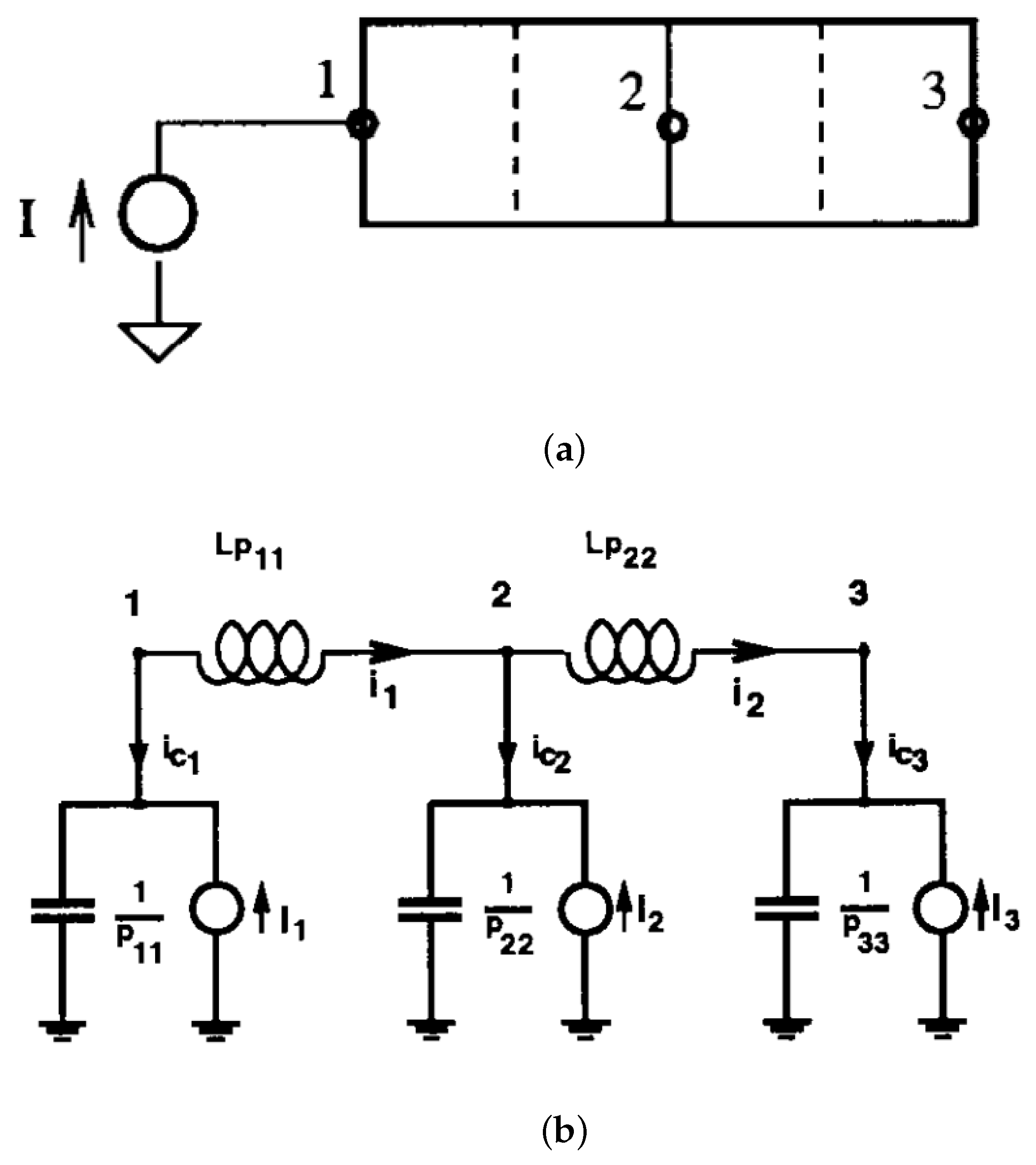
  39. Bellen, A.; Guglielmi, N.; Ruehli, A.E. Methods for linear systems of circuit delay differential equations of neutral type. IEEE Trans. Autom. Control 1999, 46, 212–216. [Google Scholar] [CrossRef]
Figure 1. (a) Metal strip with two L p cells and (b) PEEC model for the metal strip.
Mathematics 11 01199 g001
Figure 2. Output response by controller (42).
Mathematics 11 01199 g002
Figure 3. Output response by controller (42).
Mathematics 11 01199 g003
Figure 4. Output response by controller with and without time-delay term.
Mathematics 11 01199 g004
Disclaimer/Publisher’s Note: The statements, opinions and data contained in all publications are solely those of the individual author(s) and contributor(s) and not of MDPI and/or the editor(s). MDPI and/or the editor(s) disclaim responsibility for any injury to people or property resulting from any ideas, methods, instructions or products referred to in the content.

