Performance of Heat Transfer in Micropolar Fluid with Isothermal and Isoflux Boundary Conditions Using Supervised Neural Networks

Abstract

The current study delivers a numerical investigation on the performance of heat transfer and flow of micropolar fluid in porous Darcy structures with isothermal and isoflux walls (boundary conditions) of a stretching sheet. The dynamics and mechanism of such fluid flows are modelled by nonlinear partial differential equations that are reduced to a system of nonlinear ordinary differential equations by utilizing the porosity of medium and similarity functions. Generally, the explicit or analytical solutions for such nonlinear problems are hard to calculate. Therefore, we have designed a computer or artificial intelligence-based numerical technique. The reliability of neural networks using the machine learning (ML) approach is used with a local optimization technique to investigate the behaviours of different material parameters such as the Prandtl number, micropolar parameters, Reynolds number, heat index parameter, injection/suction parameter on the temperature profile, fluid speed, and spin/rotational behaviour of the microstructures. The approximate solutions determined by the efficient machine learning approach are compared with the classical Runge–Kutta fourth-order method and generalized finite difference approximation on a quasi-uniform mesh. The accuracy of the errors lies around 10⁻⁸ to 10⁻¹⁰ between the traditional analytical solutions and machine learning strategy. ML-based techniques solve different problems without discretization or computational work, and are not subject to the continuity or differentiability of the governing model. Moreover, the results are illustrated briefly to help implement microfluids in drug administering, elegans immobilization, and pH controlling processes.

1. Introduction

A fluid with microstructure or liquids that retain rigid and arbitrarily sloped atoms suspended in a viscous medium is known as a micropolar fluid. The dynamics of microfluidics have been extensively utilized due to their industrial significance, especially in thermal transport, polymer indulgence, painting material, ornament evolving, wire coatings, and drug administering [1]. The development of science and technology has sparked a surge in interest in creating new fluid types and studying how they behave in various practical geometries. Microstructured fluids react differently than conventional fluids. The traditional theory of Newtonian fluid flows is insufficient to accurately characterize the flow and heat transfer characteristics of these fluids. To explain the basic nature of these fluids, various theories have been put forth; in particular, Eringen’s [2] theory of micropolar fluids offers all the information needed to support the dynamics of such fluids. The phenomena of heat transfer are of immense importance in industrial applications. The effectiveness of thermal and cooling systems depends on the ability of fluids to transmit heat efficiently [3]. As a result, thermal enhancement has been researched extensively in recent years. Heat transfer fluid (known as HTF) is an essential part of solar thermal power plants, as it has a significant impact on the efficiency of the receiver, decides the kind of thermodynamic cycle that can be used and the level of performance it is capable of, and decides the type of thermal energy storage technology that required for implementation. H.Benoit [4] examined the liquid, gas, supercritical, two-phase, and particulate heat transfer fluids that are currently in use as well as those to be developed in the future, and presented the thermophysical properties amd correlations that can be used to determine the receiver tube–HTF heat transfer coefficients.

The two-phase magnetohydrodynamic (MHD) heat transfer flow of Newtonian fluids in MHD generators and pumps has been the subject of significant modeling work [5,6]. Many authors have contributed to these efforts. Findings have been reported for several depth-to-viscosity ratios that were considered appropriate. A. M. Siddiqui [7] examined the movement of heat that occurs between two layers of Phan–Thien–Tanner (PTT) fluids as they pass through a cylindrical conduit. M. Modak [8] studied the properties and characteristics of a stainless vertical foil of $0.15$ mm thickness utilizing various fluids, such as nanofluids $\left(A{l}_2{O}_3\right)$ and pure water, along with an infrared imaging camera. The process of heat transfer in an incompressible non-newtonian fluid under the conductance of electric charges and uniform magnetic field in the rectangular duct was studied by M. Ahmad [9]. The mathematical model of the heat transfer process in non-Newtonian micropolar fluids with viscous dissipation and power-law fluid rheology model subjected to the non-axisymmetric boundary conditions was recently studied by Ryoichi Chiba [10].

Generally, in mathematics, fluid problems are mathematically modeled as nonlinear differential equations. Because the fluids are affected by different variables, therefore, the nonlinear modeling shows the complex synergetic effects [11,12]. As has been stated in numerous studies, nonlinear models are harder to solve; therefore, various numerical, exact, and analytical approaches have been adopted by the research community [13]. N. T. El-dabe [14] investigated the changes in a chemical reaction, heat transfer, and magnetic field on the flow of a non-Newtonian fluid over the vertical cylinder using the homotopy perturbation method (HPM). M.N. Smirnova [15,16] studied the exact solution for the problem of a condensed material surface burning in a flow of oxidant in the case of the steady flame over fuel layer. Further, he utilized numerical computational methods to investigate the numerical precision and stochastic error accumulation when solving problems of detonation or deflagration combustion of gas mixtures in rocket engines [17,18]. Additionally, I. C. Liu [19] used the same method to examine how the flow and heat transfer in a thin layer on a horizontal sheet in the presence of thermal radiation are affected by varying heat flux and internal heat generation. The transfer matrix method (TMM) and variational iteration method (VIM) were applied by T.A.El-Sayed [20] to study the stability and dynamic behavior of the critical velocity by varying different parameters of a fluid flowing in a multi-span pipe. The heat transfer of a non-Newtonian fluid in an internal duct was studied by J. K. Grabski [21]. In order to achieve the general solution, the method of fundamental solutions was utilized, and radial basis function approximations were utilized in order to obtain the general solution through two different feasible methods. K. R. Raghunatha [22] implemented the Laguerre wavelet method (LWM) for numerical investigation of coupled nonlinear ordinary differential equations reduced from partial differential equations (PDEs) using Berman’s similarity transformation to represent the two-dimensional flow of a rotating micropolar fluid in a permeable channel with high mass transfer. Other techniques include the Galerkin finite element method (GFEM) [23], finite difference lattice Boltzmann method (FDLBM) [24], multi-block finite difference method [25], quadrature-based moment methods (QBMM) [26], and reproducing kernel algorithm [27].

In the recent past, researchers have focused on implementing optimization algorithms for finding solutions to nonlinear differential equations. The use of systematic procedures, strategies, disciplines, and tactics for the purpose of improving a particular process within the parameters of a project or initiative is what we mean when we talk about optimization. Adjusting a procedure in such a way that it performs more effectively than it did in the past can be achieved in a number of different ways. Simplistic examples that can assist in streamlining a workflow include deleting a step from the process, adding a step, or revising a phase that already exists in the process. Recently, optimization algorithms have been used to optimize the weights in neural networks [28,29,30]. Artificial neural networks, known as ANNs, are computational networks inspired by biological neural networks. The late nineteenth century and early twentieth century saw the beginning of the foundational research that would later become the field of artificial neural networks (ANNs). Inter-disciplinary work in the fields of physics, psychology, and neurophysiology was the primary focus of this study. This early work focused on basic theories of learning, perception, and conditioning, among other topics; nevertheless, it did not include explicit mathematical models of how neurons functioned. The study of neural networks received a new lease on life as a result of these recent advancements. Over the course of the previous two decades, a large number of academic articles have been published, and researchers have looked into a wide variety of ANN types [31,32]. The ANNs that are utilized most frequently for a wide range of issues are those that are predicated on a supervised method and consist of three layers: an input layer, a hidden layer, and an output layer. An example is shown in Figure 1. Recent applications of different types of neural networks with optimization algorithms have been widely used to solve a wide variety of problems, including heat transfer investigation of magneto-hydrodynamic fluids with equilibrium conditions using Elman neural networks [33,34], mathematical models for flow and heat-transfer analysis of a non-Newtonian fluid with axisymmetric channels and porous walls using Legendre polynomial-based neural networks [35,36], solving partial differential equations for condensation of fluid flow in a spinning cylinder using a nonlinear autoregressive exogenous model [37,38], and implementation of a feed-forward architecture neural network for thermal analysis of nanofluid flowing in a rotating system with fixed horizontal plates and subjected to external forces such as magnetic fields [39,40]. These important studies have encouraged us to incorporate and expand upon the concept of a supervised machine learning algorithm for the solutions and performance of heat transfer in micropolar fluid with isothermal and isoflux boundary conditions. Important features of the proposed study are as follows:

• In the designed scheme, a novel machine learning process is conducted by a computer that is not subject to or affected by the continuity and singularity of the differential equations.
• The machine learning techniques are applicable to multidimensional data. They can supervise the given data in an efficient manner by employing the Levenberg–Marquardt algorithm for local search optimization.
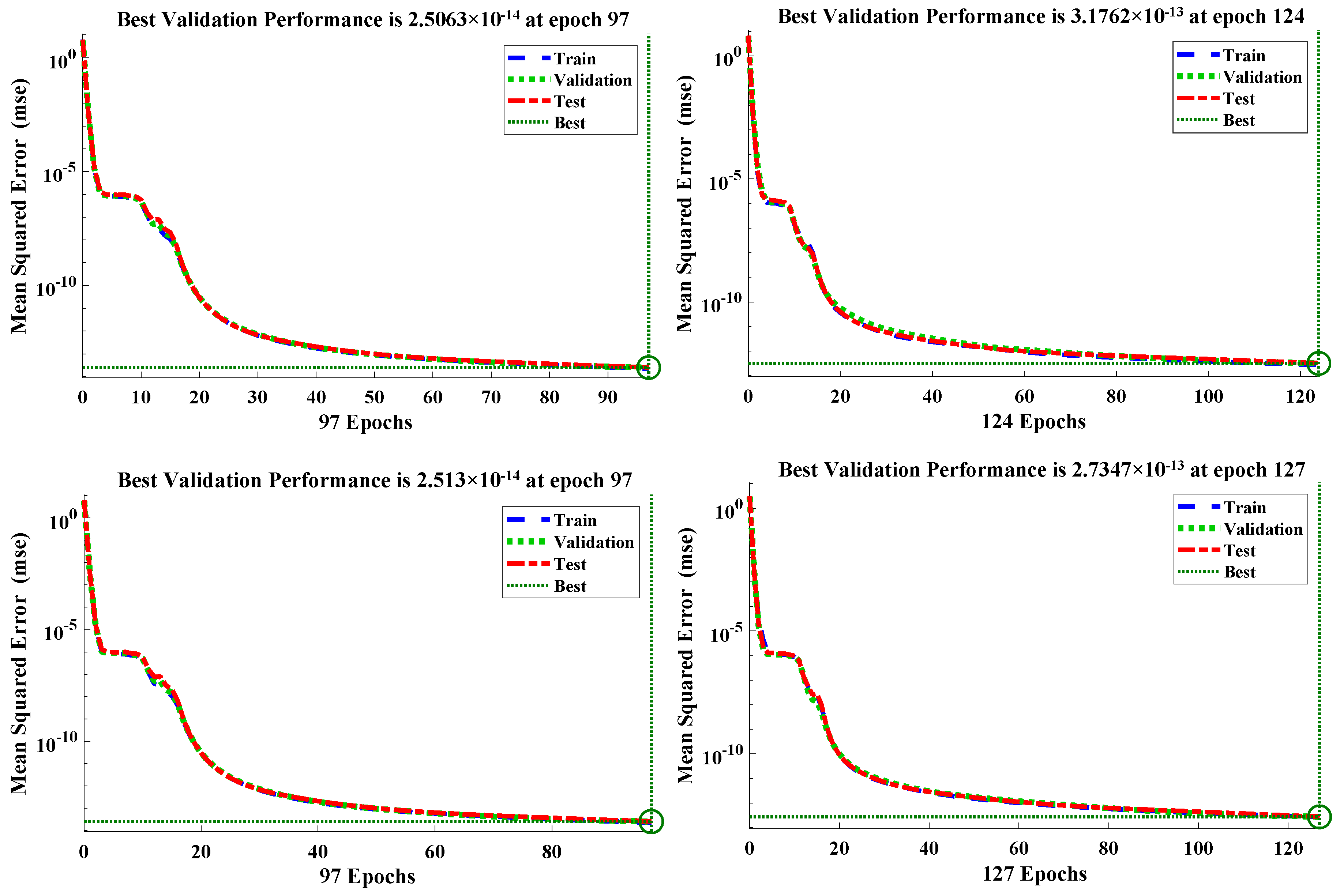
• The smooth convergence of the optimization of an objective function in terms of mean square error highlights the stability and efficiency of the designed technique.

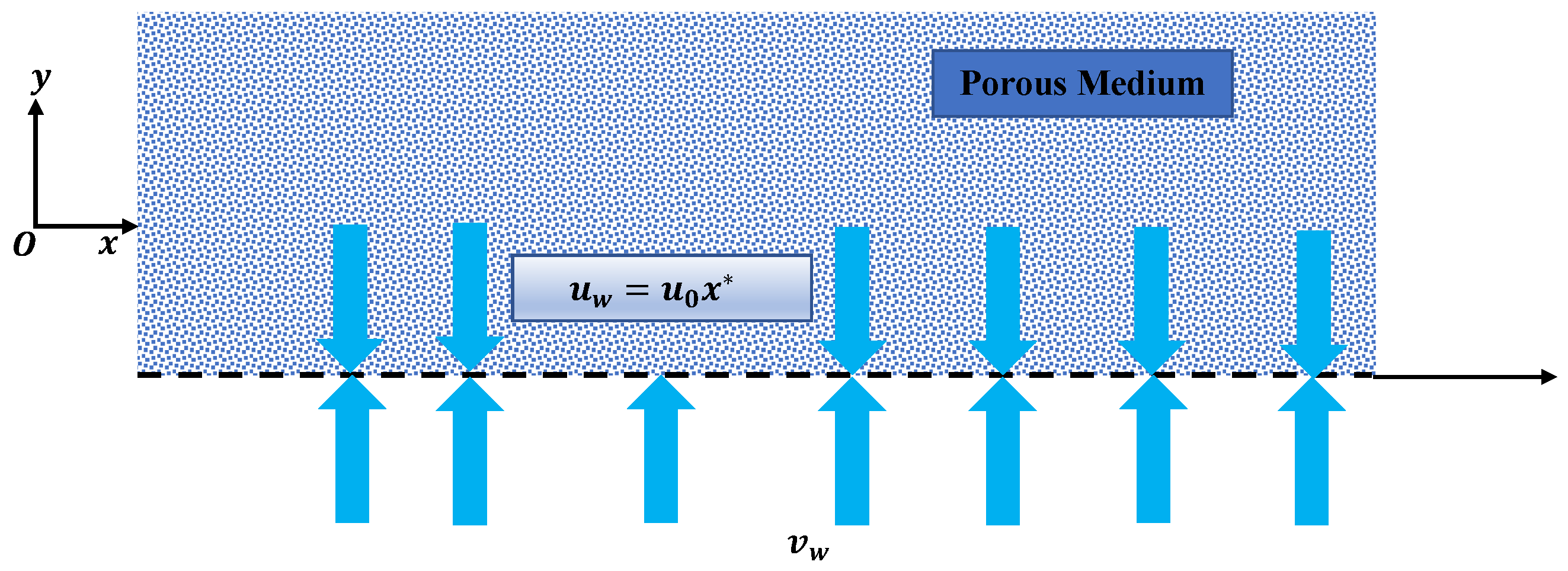
2. Governing Model of the Problem

In the classical theory of micropolar fluids, six principles are considered: three for micro-rotation and three for translation. The idea of micropolar fluid flow can be summed up as the generalization of Newtonian fluid constitutive equations such that complex microstructures such as colloidal fluids, animal blood, lubricants, muddy water, and suspension of chemicals can be briefly studied. Therefore, the mathematical structure of micropolar fluids is constructed by utilizing the principles of conservations of mass and momentum along with conservations of local angular momentum [2]. The equations are provided by

$$\nabla ·\left(\rho \mathbf{U}\right)+\frac{\partial \rho }{\partial t}=0,$$

(1)

$$\nabla (\nabla ·\mathbf{U})\left({\lambda }_{\mathrm{c}}+{\kappa }_{\mathrm{c}}+2{\mu }_{\mathrm{c}}\right)+{\kappa }_{\mathrm{c}}\nabla \times \mathbf{W}+\rho {\mathbf{f}}_{\mathrm{b}}=\rho \frac{D\mathbf{U}}{Dt}+\left({\kappa }_{\mathrm{c}}+{\mu }_{\mathrm{c}}\right)\left[\nabla \times \nabla \times \mathbf{U}\right]+\nabla P,$$

(2)

$$\nabla (\nabla ·\mathbf{W})\left({\alpha }_{\mathrm{c}}+{\beta }_{\mathrm{c}}+{\gamma }_{\mathrm{c}}\right)+{\kappa }_{\mathrm{c}}\nabla \times \mathbf{U}\mathbf{W}+\rho \mathbf{1}=\rho j\frac{D\mathbf{W}}{Dt}+\left[\nabla \times \nabla \times \mathbf{W}\right]{\gamma }_{\mathrm{c}}+2{\kappa }_{\mathrm{c}};$$

(3)

here, $\mathbf{W},\mathbf{U},{\mathbf{f}}_{\mathrm{b}},\rho ,P,\mathbf{1}$ and j are the vectors of the micro-rotation, velocity vector, force of a body, fluids density, pressure, body couple per unit of mass, and micro-inertia, respectively. Moreover, ${\mu }_{\mathrm{c}},{\lambda }_{\mathrm{c}},{\gamma }_{\mathrm{c}}$ and ${\kappa }_{\mathrm{c}}$ denote the dynamic viscosity, Stokes viscosity, spin gradient viscosity, and vortex viscosity, respectively, while ${\alpha }_{\mathrm{c}}$ and ${\beta }_{\mathrm{c}}$ are the material constants.

Consider a micropolar fluid flow in a homogenous, permeable, and porous material with permeability K over a porous stretched sheet, as schematized in Figure 2. The flow is assumed to be two-dimensional (2D), incompressible, and independent of time, while the body force and body couple are neglected. The flow of the fluid is caused by a sheet that is permeable, has a length of L, and is expanding linearly along the x-axis. The y-axis runs in a direction that is orthogonal to the sheet. The expression $u_w=u_{0}x/L$ describes the linear velocity profile of the flow along the sheet. Using the above assumption, Equations (1)–(3) are reduced to [41]

$$\frac{\partial u}{\partial x}+\frac{\partial v}{\partial y}=0,$$

(4)

$$\left({\mu }_{\mathrm{c}}+{\kappa }_{\mathrm{c}}\right)\left(\frac{{\partial }^{2}u}{\partial x^2}+\frac{{\partial }^{2}u}{\partial y^2}\right)+{\kappa }_{\mathrm{c}}\frac{\partial {\omega }_3}{\partial y}-\frac{{\mu }_{\mathrm{c}}}{K}u=\rho \left(u\frac{\partial u}{\partial x}+v\frac{\partial u}{\partial y}\right),$$

(5)

$${\gamma }_{\mathrm{c}}\frac{{\partial }^2{\omega }_3}{\partial y^2}-2{\kappa }_{\mathrm{c}}{\omega }_3+{\kappa }_{\mathrm{c}}\frac{\partial u}{\partial x}=\rho jv\frac{\partial {\omega }_3}{\partial y},$$

(6)

where u and v are the vertical and orthogonal components of the fluid velocity along the x and y axis, respectively, and ${\omega }_3$ denotes the component of the micro-rotation that is perpendicular to the $xy$-plane. If T denotes the temperature of the fluid, then the energy equation is stated as [41] follows:

$$u\frac{\partial T}{\partial x}+v\frac{\partial T}{\partial y}={\alpha }_{\mathrm{eff}}\frac{{\partial }^{2}T}{\partial y^2},$$

(7)

where ${\alpha }_{\mathrm{eff}}$ highlights the effectiveness of thermal diffusivity. The corresponding hydrodynamic boundary conditions are then

$$u\left(x^{*},0\right)=U_0{x}^{*},u\left(x^{*},\infty \right)=0$$

$$v\left(x^{*},0\right)=v_w,$$

$${\omega }_3\left(x^{*},0\right)=-m\frac{\partial u}{\partial y},{\omega }_3\left(x^{*},\infty \right)=0,$$

where $v_w$ is the rate of mass transfer at the edge of a sheet, $U_0$ is a constant representing the coefficient of the wall velocity, and $m\in [0,1]$. Different cases and types of flows based on values of m have been suggested in various studies [42,43]. Furthermore, $x^{*}=\frac{x}{L}$ is a non-dimensional x-coordinate based on the length L of the permeable sheet. The scenario $m=1$ is used to model the turbulent boundary layer flows [44]. These thermal boundary conditions for power law temperature and heat flux are taken into account as follows:

$$T\left(x^{*},0\right)=T_{\infty }+T_0{\left(x^{*}\right)}^s,T\left(x^{*},\infty \right)=T_{\infty },$$

(8)

$$-{\left.\tau \frac{\partial T}{\partial y}\right|}_{\left(x^{*},0\right)}=q_0{\left(x^{*}\right)}^s,T\left(x^{*},\infty \right)=T_{\infty }$$

(9)

where the coefficient of wall temperature is shown by $T_0$, $T_{\infty }$ denotes the temperature far away from the sheet, $q_0$ is the coefficient of heat flux at the edge of the sheet, $\tau$ is the thermal conductivity of the medium, and s is the index of the power law. Furthermore, in order to transform the partial differential equations into the system of ordinary differential equations, the following similarity functions are defined:

$$\eta =\frac{y}{\sqrt{K}},\psi =U_0{x}^{*}\sqrt{K}f\left(\eta \right),$$

$$u=U_0{x}^{*}{f}^{\prime }\left(\eta \right),v=-\frac{U_0}{L}\sqrt{K}f\left(\eta \right),{\omega }_3=\frac{U_0{x}^{*}}{\sqrt{K}}H\left(\eta \right).$$

where $v=-\partial \psi /\partial x,u=\partial \psi /\partial y,$ $\psi$ is stream function, and $f^{\prime }=\mathrm{d}f/\mathrm{d}\eta$. Then, using the above assumptions in Equation (5), (7) can be reduced to the following system of ODEs:

$$\left(c_1+1\right)f^{‴}+\left(f^{″}f-{f^{\prime }}^2\right)R_{\mathrm{e}}-f^{\prime }+c_1{H}^{\prime }=0,$$

(10)

$$H^{″}-c_1{c}_2\left(f^{″}-2H\right)-c_3\left(f^{\prime }H-f{H}^{\prime }\right)=0,$$

(11)

$${\theta }^{″}+P_{\mathrm{r}}{R}_{\mathrm{e}}\left(f{\theta }^{\prime }-s{f}^{\prime }\theta \right)=0,$$

(12)

where $P_{\mathrm{r}}$ is the Prandtl number and $R_{\mathrm{e}}$, $c_1,c_2$, and $c_3$ are the Reynolds number and non-dimensionless material constants, respectively, which are defined as

$$R_{\mathrm{e}}=\frac{\rho U_{0}K}{L{\mu }_{\mathrm{c}}},c_1=\frac{{\kappa }_{\mathrm{c}}}{{\mu }_{\mathrm{c}}},c_2=\frac{{\kappa }_{\mathrm{c}}{\mu }_{\mathrm{c}}}{{\gamma }_{\mathrm{c}}},c_3=\frac{\rho j{\kappa }_{\mathrm{c}}{\mu }_{\mathrm{c}}}{{\gamma }_{\mathrm{c}}}.$$

Now, the corresponding boundary conditions for the governing model of the micropolar fluid are defined as follows:

$$f^{\prime }\left(0\right)=1,f\left(0\right)=\lambda ,f^{\prime }(\infty )=0,H\left(0\right)=0,H(\infty )=0$$

(13)

$$\theta =1,\mathrm{at}\eta =0,\theta =0\mathrm{at}\eta \to \infty ,$$

(14)

$${\theta }^{\prime }=-1\mathrm{at}\eta =0,{\theta }^{\prime }=0\mathrm{at}\eta \to \infty .$$

(15)

The isothermal and isoflux conditions are shown by Equations (14) and (15). Moreover, $\lambda =-v_{\mathrm{w}}L/U_0\sqrt{K}$ is an injection/suction parameter.

3. Method of Solution

This section provides a description of the methods and materials utilised in this work for the purpose of predicting numerical solutions for a micropolar fluid flowing over a stretched sheet with isothermal and isoflux boundary conditions.

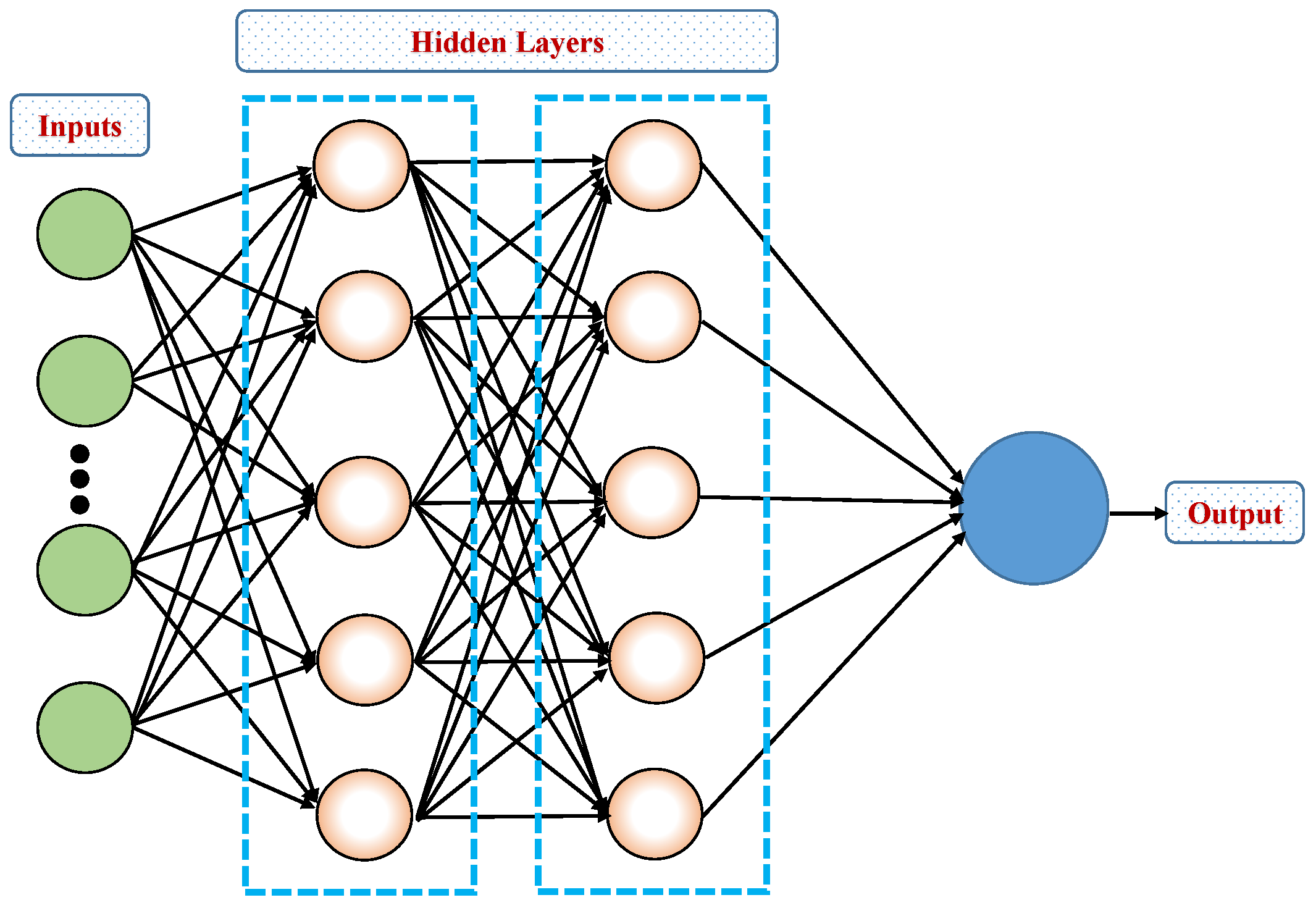
3.1. Artificial Neural Networks

ANN is an abbreviation for an architecture that is parallel in nature, and is inspired by the method in which central nervous system processing occurs. A neural network is a collection of computing devices that are coupled to provide a computer with the ability to learn and behave in a manner similar to that of a brain. Neuroscientists researching neurons in the brains of individuals and animals developed the concept of neural networks while conducting related their research. The field of artificial intelligence is an ongoing effort to endow computing devices with the ability to interpret data and arrive at conclusions in a manner that is comparable to that of human beings. An advanced concept within this field is known as an artificial neural network, and it is part of the field of artificial intelligence. Although there are many other kinds of ANN designs, the one that is used the most frequently is called a multi-layer feed-forward neural network, or MLP [45]. Mathematically, the structure of ANN can be defined as

$$W\left(\eta \right)=\sum _{j=1}^N{\widehat{\alpha }}_{j}f\left({\widehat{b}}_j\eta +{\widehat{c}}_j\right),$$

(16)

where ${\widehat{\alpha }}_j,{\widehat{b}}_j$, and ${\widehat{c}}_j$ are the weights or neurons that are optimized during the optimization process; in this study, tangent sigmoid is used as an activation function, which is denoted by f and defined as follows:

$$f\left(\eta \right)=\frac{e^{\eta }-e^{-\eta }}{e^{\eta }+e^{-\eta }}.$$

(17)

The hyperbolic tangent activation function is referred to simply as the Tanh (sometimes “tanh” or “TanH”) function. It is comparable to the sigmoid activation function, to the point where of even having an identical S-shaped curve. Any real value can be used as an input for the function, and it returns values in the range from −1 to 1.

3.2. Dataset

In this section, we discuss the dataset used for supervised learning of the solutions to the micropolar fluid problem with isothermal and isoflux conditions. Different cases were examined in this work to study the influential performance of the velocity, acceleration, temperature, and micro-rotation. The different cases studied in this paper are provided in

Table 1. The detailed overview of the cases studied in this paper.

Fixed Parameters						Variations
${\mathit{c}}_{\mathbf{1}}$	${\mathit{c}}_{\mathbf{2}}$	${\mathit{c}}_{\mathbf{3}}$	$\mathit{\lambda }$	${\mathit{P}}_{\mathit{r}}$	${\mathit{R}}_{\mathit{e}}$	${\mathit{c}}_{\mathbf{1}}$	$\mathit{\lambda }$	${\mathit{P}}_{\mathit{r}}$	${\mathit{R}}_{\mathit{e}}$	$\mathit{s}$
0.5	0.1	0.5	0.0	1.0	1.0	0.5	−0.2	0.5	0.0	0.0
						1.0	−0.1	1.0	1.0	1.0
						1.5	0.0	5.0	2.0	2.0
						2.0	0.1	10.0	3.0	3.0
						2.5	0.2	15.0	4.0	4.0

. For the supervised learning, the dataset was generated for all these cases using the numerical solver “ND-Solve” in Mathematica running the Runge–Kutta algorithm of order 4.

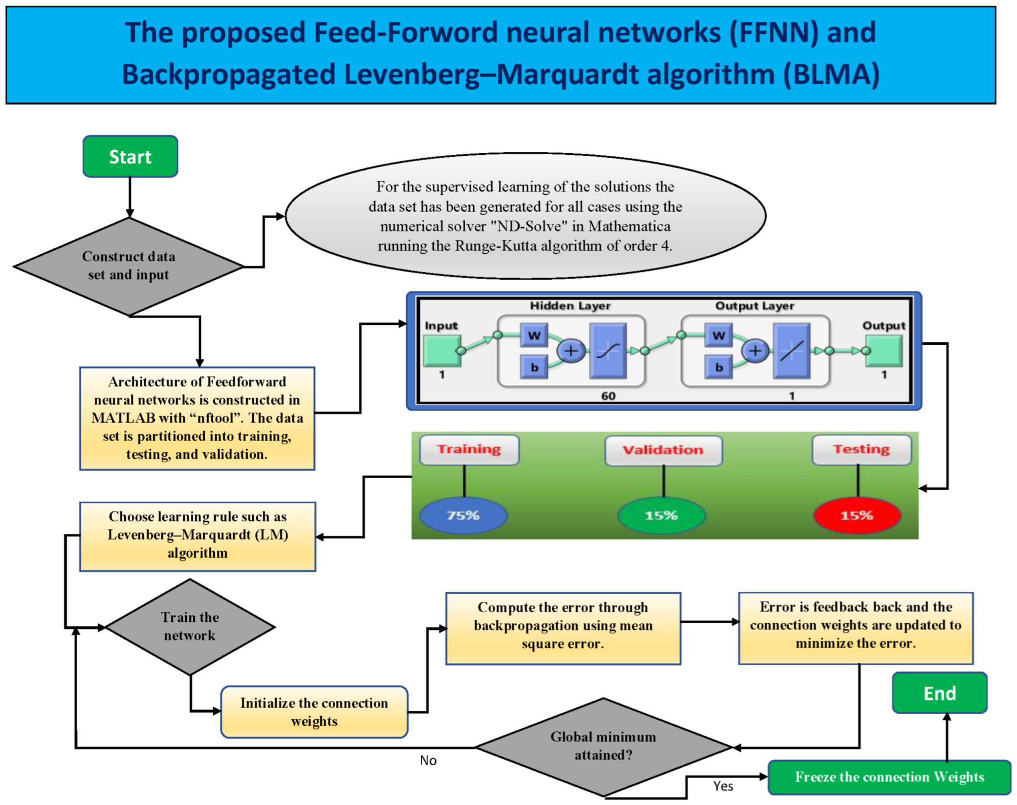
3.3. ANN with Levenberg–Marquardt Algorithm

The field of artificial intelligence that studies how machines can be taught to learn from the data provided to them is known as machine learning. Machine learning algorithms are computing methods that “learn” information directly from data without depending on a preconceived equation as a model. These algorithms are used in artificial intelligence (AI). When there are more data points available for learning, these algorithms are able to make dynamic improvements to their performance. Furthermore, the operational phases of the method (FFNN-BLMA) that is being proposed here is discussed below and shown in Figure 3.

• The initial dataset is generated by a numerical solver such as the Runge–Kutta method for the supervised procedure of the machine learning algorithm. This step is used to determine how well the model performs on real-world datasets.
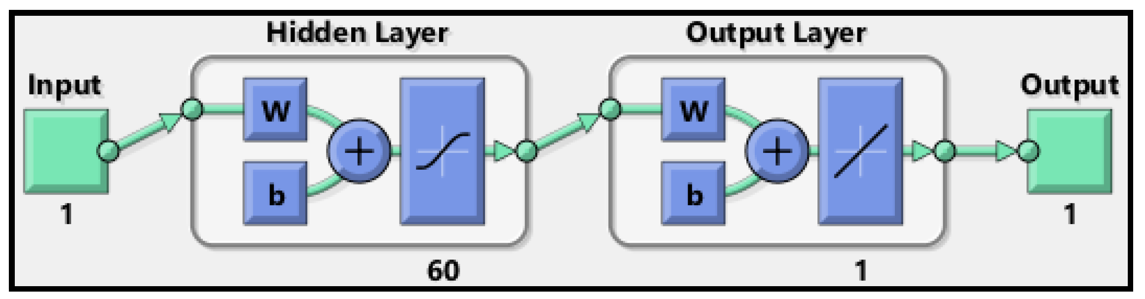
• Further, the neural network model is constructed using the NFTOOL in MATLAB to contrive the feed-forward architecture of an artificial neural network (FFNN) with 60 neurons in the hidden layer, as shown in Figure 4. The dataset of 1001 points obtained in the first step is provided to the FFNN as targeted data. In the FFNN model, the dataset is partitioned into training, testing, and validation with respective weightings of $75\%$ and $15\%$.
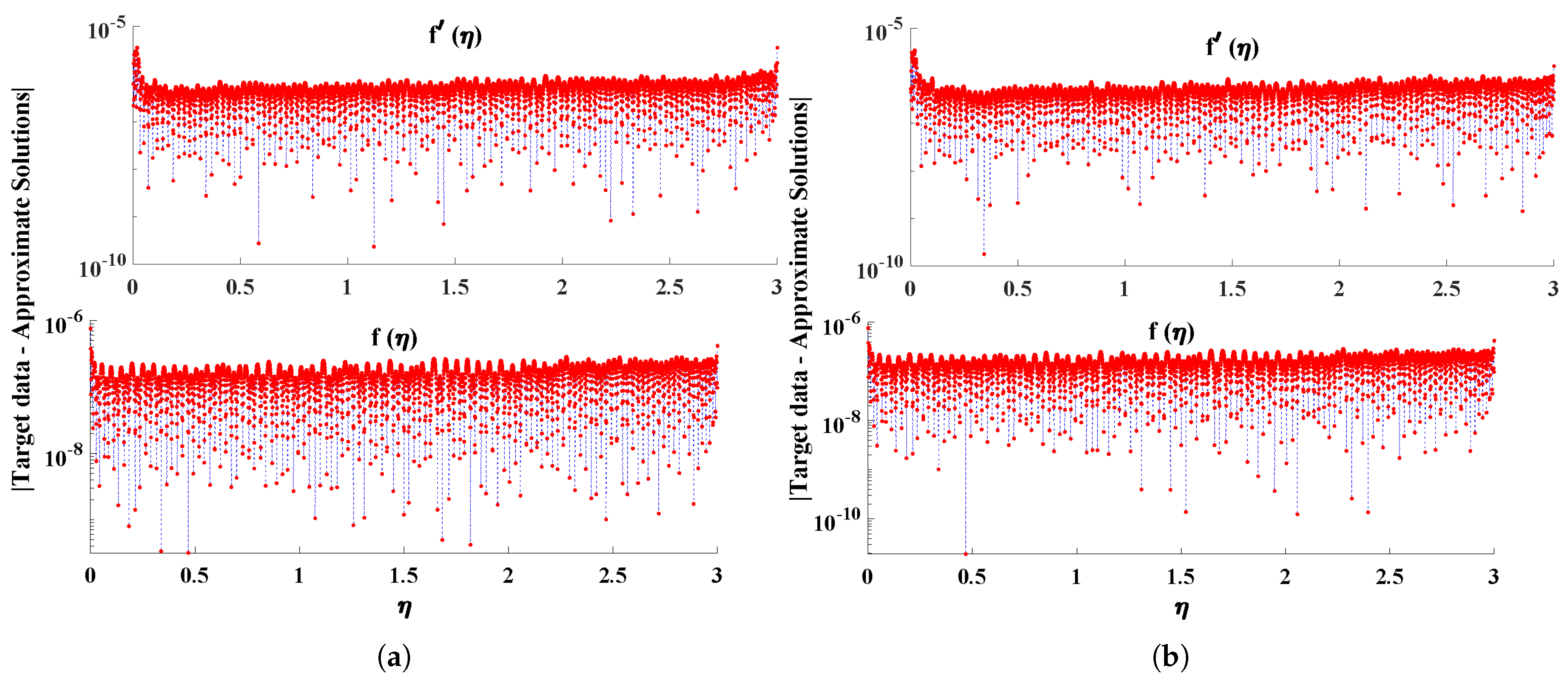
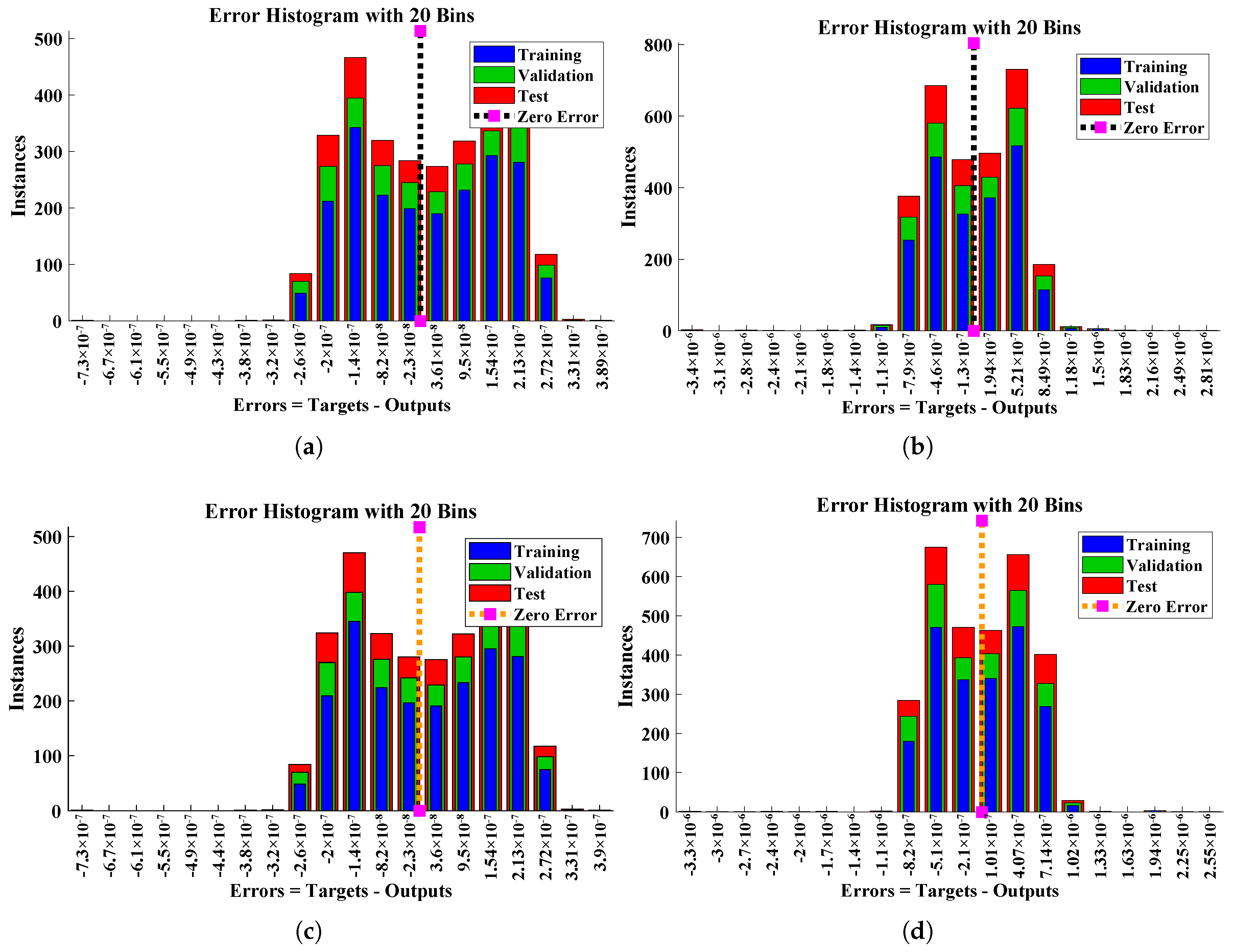
• The mean squared error (MSE) is often used as the objective function in feed-forward neural network (FFNN) models. The MSE measures the average difference between the predicted output and the actual output. The objective is to minimize this error during the training process to improve the model’s accuracy. Mathematically, the fitness function $\left(E\right)$ can be written as

  $$E=\frac{1}{m}\sum _{i=1}^m{\left({\widehat{y}}_i-y_i\right)}^2,$$

  (18)

  where $y_i$ refers to the predicted value of the target variable based on the input variables for the $i^{th}$ sample in a dataset.
• The Levenberg–Marquardt algorithm is an optimization method used to minimize a non-linear least-squares function. It is a combination of the gradient descent and the Gauss–Newton method, and uses a damping parameter to control the trade-off between exploration and exploitation. It is widely used in applications such as curve fitting, training artificial neural networks, and solving nonlinear systems of equations. It is an efficient method for finding the optimal weights associated with the predicted solution in Equation (18). This algorithm adjusts the weights until the error between the predicted and actual solution is minimized. The detailed mathematical operational work of LM algorithm can be found in [46].

4. Results and Discussion

In this paper, we investigate the fluid flow, heat transfer, and micro-rotation of a micro-fluid by incorporating a machine learning strategy. The results of the proposed technique are disclosed in Tables. The values for the flow speed and acceleration of the micropolar fluid with isothermal and isoflux boundary conditions are presented in

Table 2. Examination of the absolute errors and the predicted solutions calculated by the designed framework for the fluid speed with isothermal boundary conditions.

	RKM	NSFDA	FFDNN-BLMA	NSFDA	FFDNN-BLMA
0.00	0.0000000	0.0000000	0.0000008	0.0000000	$7.587883\times {10}^{-07}$
0.50	0.3803383	0.3803700	0.3803385	$3.165134\times {10}^{-05}$	$1.432999\times {10}^{-07}$
1.00	0.5943089	0.5943500	0.5943088	$4.111222\times {10}^{-05}$	$1.299534\times {10}^{-07}$
1.50	0.7144438	0.7145000	0.7144438	$5.617930\times {10}^{-05}$	$1.189993\times {10}^{-09}$
2.00	0.7816255	0.7816900	0.7816256	$6.454517\times {10}^{-05}$	$9.794322\times {10}^{-08}$
2.50	0.8189137	0.8189800	0.8189139	$6.634720\times {10}^{-05}$	$2.040021\times {10}^{-07}$
3.00	0.8393279	0.8393900	0.8393275	$6.212871\times {10}^{-05}$	$4.188753\times {10}^{-07}$

,

Table 3. Depiction and statistical evaluation of the proposed solutions with recent techniques and overview of the absolute errors of the acceleration with isothermal boundary conditions.

	RKM	NSFDA	FFDNN-BLMA	NSFDA	FFDNN-BLMA
0.0	1.0000000	1.0000000	0.9999994	0.0000000	$6.156236\times {10}^{-07}$
0.5	0.5628819	0.5628700	0.5628819	$1.192400\times {10}^{-05}$	$5.782647\times {10}^{-08}$
1.0	0.3163963	0.3163900	0.3163969	$6.297000\times {10}^{-06}$	$6.152475\times {10}^{-07}$
1.5	0.1773311	0.1773200	0.1773308	$1.108800\times {10}^{-05}$	$2.928017\times {10}^{-07}$
2.0	0.0988346	0.0988300	0.0988342	$4.581000\times {10}^{-06}$	$4.153778\times {10}^{-07}$
2.5	0.0545187	0.0545100	0.0545193	$8.738000\times {10}^{-06}$	$5.406642\times {10}^{-07}$
3.0	0.0295128	0.0295000	0.0295164	$1.283600\times {10}^{-05}$	$3.535229\times {10}^{-06}$

,

Table 4. Evaluation of the error values of the approximate solutions estimated by the designed method for the fluid speed with isoflux boundary conditions.

	RKM	NSFDA	FFDNN-BLMA	NSFDA	FFDNN-BLMA
0.0	0.0000000	0.0000000	0.0000008	0.00000000	$7.602287\times {10}^{-07}$
0.5	0.3802468	0.3802400	0.3802469	$6.792000\times {10}^{-06}$	$1.430769\times {10}^{-07}$
1.0	0.5940108	0.5939800	0.5940107	$3.079400\times {10}^{-05}$	$1.294432\times {10}^{-07}$
1.5	0.7139011	0.7138400	0.7139011	$6.106700\times {10}^{-05}$	$3.144573\times {10}^{-09}$
2.0	0.7808526	0.7807800	0.7808527	$7.259700\times {10}^{-05}$	$1.002245\times {10}^{-07}$
2.5	0.8179594	0.8178900	0.8179596	$6.943800\times {10}^{-05}$	$2.029088\times {10}^{-07}$
3.0	0.8382604	0.8382200	0.8382600	$4.038600\times {10}^{-05}$	$4.193764\times {10}^{-07}$

and

Table 5. Evaluation of the error values of the approximate solutions estimated by the designed method for the acceleration of fluid flow with isoflux boundary conditions.

	RKM	NSFDA	FFDNN-BLMA	NSFDA	FFDNN-BLMA
0.0	1.0000000	1.0000000	0.9999995	0.00000000	$5.331604\times {10}^{-07}$
0.5	0.5625532	0.5625100	0.5625531	$4.321144\times {10}^{-05}$	$7.240753\times {10}^{-08}$
1.0	0.3159240	0.3158700	0.3159246	$5.400470\times {10}^{-05}$	$5.942010\times {10}^{-07}$
1.5	0.1768421	0.1767900	0.1768416	$5.209980\times {10}^{-05}$	$4.668274\times {10}^{-07}$
2.0	0.0984144	0.0983900	0.0984139	$2.440139\times {10}^{-05}$	$5.325018\times {10}^{-07}$
2.5	0.0542198	0.0542200	0.0542204	$2.136859\times {10}^{-07}$	$5.898603\times {10}^{-07}$
3.0	0.0293613	0.0294000	0.0293629	$3.873600\times {10}^{-05}$	$1.598029\times {10}^{-06}$

, respectively. The validation of the predicted solution is demonstrated by a comparison with the most recent methods, such as the RK method and generalized finite difference approximation [41]. The minimum absolute errors between the predicted solution with supervised machine learning are observed in comparison to the latest methodologies available in the literature. The targeted values or supervised data overlap to 7 to 9 decimal places. Furthermore, the absolute difference between the predicted values of the velocity and acceleration with isothermal and isoflux boundary conditions are shown in Figure 5. It can be observed that the mean values of the absolute errors lie between ${10}^{-7}$ to ${10}^{-8}$. Moreover, around $95\%$ of the datapoints from a total of 3001 points are less than ${10}^{-8}$, which reflects the estimation power as well as the precision of the methods of machine learning. The error estimation in the predicted values of the targeted data, validation data, and testing data are illustrated in Figure 6. An adaptive training algorithm based on the Levenberg–Marquardt method was used to train a neural network, with the convergence analysis shown in Figure 7. After each iteration of training, the objective function value obtained by backpropagation was compared to the value generated by the initial network. Each time a new iteration began and a weight update was performed, a new weight matrix was derived from either the step-by-step learning or from calculation of the local optima. The blue, green, and red lines show the MSE for the test, validation, and training sets, respectively. In this study, we were able to implement an adaptive learning algorithm for our neural networks as well as to show that these networks can learn quickly and accurately when provided with a set of data.

The mathematical model of a microfluid was analyzed in detail, with an emphasis on the changes in different parameters, i.e., $0.5\le c_1\le 2.5$, $-0.2\le \lambda \le 0.2$, $0.5\le P_r\le 15.0$, $0\le R_e\le 4$, and $0\le s\le 4.0$, on the velocity, temperature, micro-rotations of the fluid. In order to analyze the detailed changes taking place in the mathematical model of the microfluid, graphical analysis was used extensively. The effects of the injection/suction parameter on the velocity and microrotation of the micropolar fluid with different boundary conditions can be seen in Figure 8. In the figure, $\lambda >0$ refers to suction, while $\lambda <0$ indicates injection and $\lambda =0$ means no suction/injection in the flow domain. It can be seen that when $\lambda$ increases, $f^{\prime }\left(\eta \right)$ decreases; this is due to the fact the temperature of a fluid decreases that when fluid particles are injected into a porous medium, which causes the weakening of the convection current, in turn decreasing the moments of the particles. Moreover, the increase in $\lambda$ causes a decrease in the micro-rotation of the fluid, as depicted in Figure 8b,d. It can be seen that the effect of the boundaries on velocity is almost negligible, while there are significant changes in micro-rotation.

The changes in Reynolds number $\left(R_e\right)$ between the different profiles of the micro-polar fluid are demonstrated in Figure 9. The Reynolds number is a dimensionless number that relates the inertial forces and viscous forces. The Reynolds number defines the ratio of viscosity to inertia, and is used to categorize fluid systems in which viscosity is important for controlling the flow volume or velocity of a fluid. Thus, an increase in the value of this parameter decreases the value of the flow speed, while boundary layer thickness is reduced with an increasing value of $\left(R_e\right)$ under isothermal and isoflux boundary conditions, as shown in Figure 9. The effect on the micro-rotation $H\left(\eta \right)$ is shown in Figure 9b,d for isothermal and isoflux boundary conditions. In both cases, the micro-rotation is increased near the boundary and gradually decreases when the distance between fluid particles and the wall or edge of the sheet increases.

The influence that the Prandtl number $\left(P_r\right)$ and the heat index parameter have on the temperature profile of the micropolar fluid can be seen in Figure 10. The Prandtl number is a dimensionless number that determines the intrinsic property of a fluid, and is defined as the ratio of the momentum diffusivity (or kinematic viscosity) to the thermal diffusivity of the fluid. As the Pr value increases, the temperature continues to drop. The thickness of the thermal boundary layer is decreased whenever the Prandtl number is increased. In problems involving heat transfer, $P_r$ is the variable that determines the relative thickness of the momentum and thermal boundary layers. When Pr is low, heat diffuses swiftly in comparison to the velocity, which implies that for liquid metals the thickness of the thermal boundary layer is much greater than that of the momentum boundary layer. When $P_r$ is high, heat diffuses slowly in comparison to the momentum. Fluids with lower Prandtl values have greater thermal conductivities (and thicker thermal boundary layer structures), which means that heat can diffuse out from the sheet more quickly than it does for fluids with higher Pr (thinner boundary layers). Therefore, the Prandtl number may be used to ascertain the rate of cooling that takes place in conducting flows. Similarly, an increase in heat index parameters causes the temperature of the micropolar fluid to decrease for different conditions, as depicted in Figure 10b,d. This comparison shows that the intensity of declination in the temperature profile of the fluid is higher with the isothermal boundary condition than the isoflux boundary condition. Figure 11a,c illustrates the relationship between an increase in the value of the micropolar parameter $c_1$ and a corresponding rise in the boundary layer thickness of the fluid flow. The fluid’s velocity increases with the same ratio and intensity for both isothermal and isoflux conditions. At the same time, a decline is observed in the temperature profile of the fluid.

5. Performance Indices and Statistical Evaluation

The main objective of this paper is to propose FFDNN-BLMA for solving nonlinear complex problems such as heat transfer in micropolar fluids with isothermal and isoflux boundary conditions. This algorithm is available as part of MATLAB, and has been used by many researchers for solving different types of problems. In this study, high-quality solutions have been obtained, as presented in the previous section, and have been compared with those of two other algorithms. In this section, the stability, consistency, and accuracy measures are established and the performance of the proposed algorithm is analyzed by incorporating the proposed technique for multiple runs on the same dataset for different cases. Different measures are defined to validate the quality of the predicted solutions. The formulation of these measures is as follows:

$$\left[{\mathrm{TIC}}_f,{\mathrm{TIC}}_H,{\mathrm{TIC}}_{\theta }\right]={\left[\begin{array}{c}\frac{\sqrt{\frac{1}{\Omega }{\sum }_{i=1}^{\Omega }{\left(f\left(\eta \right)-\widehat{f}\left(\eta \right)\right)}^2}}{\sqrt{\frac{1}{\Omega }{\sum }_{i=1}^{\Omega }{\left(f\left(\eta \right)\right)}^2}+\sqrt{\frac{1}{\Omega }{\sum }_{i=1}^{\Omega }{\left(\widehat{f}\left(\eta \right)\right)}^2}},\\ \\ \frac{\sqrt{\frac{1}{\Omega }{\sum }_{i=1}^{\Omega }{\left(H\left(\eta \right)-\widehat{H}\left(\eta \right)\right)}^2}}{\sqrt{\frac{1}{M}{\sum }_{i=1}^{\Omega }{\left(H\left(\eta \right)\right)}^2}+\sqrt{\frac{1}{\Omega }{\sum }_{i=1}^{\Omega }{\left(\widehat{H}\left(\eta \right)\right)}^2}},\\ \\ \frac{\sqrt{\frac{1}{\Omega }{\sum }_{i=1}^M{\left(\theta \left(\eta \right)-\widehat{\theta }\left(\eta \right)\right)}^2}}{\sqrt{\frac{1}{\Omega }{\sum }_{i=1}^{\Omega }{\left(\theta \left(\eta \right)\right)}^2}+\sqrt{\frac{1}{\Omega }{\sum }_{i=1}^{\Omega }{\left(\widehat{\theta }\left(\eta \right)\right)}^2}},\end{array}\right]}^t,$$

(19)

$$\left[{\mathrm{MAD}}_f,{\mathrm{MAD}}_H,{\mathrm{MAD}}_{\theta }\right]={\left[\begin{array}{c}\frac{1}{\Omega }\sum _{i=1}^{\Omega }\left|f\left(\eta \right)-\widehat{f}\left(\eta \right)\right|,\hfill \\ \\ \frac{1}{\Omega }\sum _{i=1}^{\Omega }\left|H\left(\eta \right)-\widehat{H}\left(\eta \right)\right|,\hfill \\ \\ \frac{1}{\Omega }\sum _{i=1}^{\Omega }\left|\theta \left(\eta \right)-\widehat{\theta }\left(\eta \right)\right|,\hfill \end{array}\right]}^t$$

(20)

$$\left[{\mathrm{RMSE}}_f,{\mathrm{RMSE}}_H,{\mathrm{RMSE}}_{\theta }\right]={\left[\begin{array}{c}\sqrt{\frac{{\sum }_{i=1}^{\Omega }{\left(f\left(\eta \right)-\widehat{f}\left(\eta \right)\right)}^2}{M}},\hfill \\ \\ \sqrt{\frac{{\sum }_{i=1}^{\Omega }{\left(H\left(\eta \right)-\widehat{H}\left(\eta \right)\right)}^2}{\Omega }},\hfill \\ \\ \sqrt{\frac{{\sum }_{i=1}^{\Omega }{\left(\theta \left(\eta \right)-\widehat{\theta }\left(\eta \right)\right)}^2}{\Omega }},\hfill \end{array}\right]}^t$$

(21)

$$\left[ENS{E}_f,ENS{E}_H,ENS{E}_{\theta }\right]=\left[\begin{array}{c}1-NS{E}_f,1-NS{E}_H,1-NS{E}_{\theta }\hfill \end{array}\right],$$

(22)

where NSE is defined as

$$\left[{\mathrm{NSE}}_f,{\mathrm{NSE}}_H,{\mathrm{NSE}}_{\theta }\right]={\left[\begin{array}{c}1-\frac{{\sum }_{i=1}^{\Omega }{\left(f\left(\eta \right)-\widehat{f}\left(\eta \right)\right)}^2}{{\sum }_{i=1}^{\Omega }{\left(f\left(\eta \right)-\overline{f}\left(\eta \right)\right)}^2},\hfill \\ \\ \overline{f}\left(\eta \right)=\frac{1}{\Omega }\sum _{i=1}^{\Omega }f\left(\eta \right),\hfill \\ \\ 1-\frac{{\sum }_{i=1}^{\Omega }{\left(H\left(\eta \right)-\widehat{H}\left(\eta \right)\right)}^2}{{\sum }_{i=1}^{\Omega }{\left(H\left(\eta \right)-\overline{H}\left(\eta \right)\right)}^2},\hfill \\ \\ \overline{H}\left(\eta \right)=\frac{1}{\Omega }\sum _{i=1}^{\Omega }H\left(\eta \right),\hfill \\ \\ 1-\frac{{\sum }_{i=1}^{\Omega }{\left(\theta \left(\eta \right)-\widehat{\theta }\left(\eta \right)\right)}^2}{{\sum }_{i=1}^{\Omega }{\left(\theta \left(\eta \right)-\overline{\theta }\left(\eta \right)\right)}^2},\hfill \\ \\ \overline{\theta }\left(\eta \right)=\frac{1}{\Omega }\sum _{i=1}^{\Omega }\theta \left(\eta \right),\hfill \end{array}\right]}^t$$

(23)

where $\Omega$ shows the number of mesh points and ENSE, RMSE, TIC, and MAD are defined as the error in terms of the Nash–Sutcliffe efficiency, root mean square error, Theil’s inequality coefficient, and mean absolute deviation. These performance measures have been previously used by many different researchers in order to validate their studies [47]. In this study, the initial generated datasets were utilized, and the proposed technique was implemented for ten independent runs in order to determine the minimum, average, and standard deviations of the predicted solutions.

The behavior of the validation data, testing data, training data, relative error (RE), RMSE, ENSE, MAD, and TIC in the predicted solutions for velocity and acceleration of the micropolar fluid in each individual run is shown in Figure 12 and Figure 13 for the isothermal and isoflux conditions, respectively. The streamlined values for each run reflect the stability of the predicted solutions. The mean values as shown in

Table 6. Statistical analysis of the values of the validation, testing, and training data along with performance measures computed for the error in the solutions of velocity and acceleration for the micropolar fluid flow with isothermal boundary conditions.

	Training	Validation	Testing	MAD	TIC	RMSE	RE	ENSE
Minimum	$2.26\times {10}^{-14}$	$2.51\times {10}^{-14}$	$2.56\times {10}^{-14}$	$1.35\times {10}^{-07}$	$4.38\times {10}^{-09}$	$1.53\times {10}^{-07}$	$1.97\times {10}^{-07}$	$1.10\times {10}^{-09}$
Mean	$3.28\times {10}^{-12}$	$3.93\times {10}^{-12}$	$4.01\times {10}^{-12}$	$1.29\times {10}^{-06}$	$4.32\times {10}^{-08}$	$1.51\times {10}^{-06}$	$1.96\times {10}^{-06}$	$1.53\times {10}^{-07}$
Stand. Dev.	$3.37\times {10}^{-12}$	$4.09\times {10}^{-12}$	$4.18\times {10}^{-12}$	$9.85\times {10}^{-07}$	$3.33\times {10}^{-08}$	$1.16\times {10}^{-06}$	$1.51\times {10}^{-06}$	$1.56\times {10}^{-07}$
Minimum	$2.72\times {10}^{-13}$	$3.18\times {10}^{-13}$	$3.21\times {10}^{-13}$	$4.55\times {10}^{-07}$	$3.41\times {10}^{-08}$	$5.36\times {10}^{-07}$	$8.28\times {10}^{-07}$	$9.36\times {10}^{-09}$
Mean	$2.34\times {10}^{-12}$	$2.94\times {10}^{-12}$	$2.82\times {10}^{-12}$	$1.22\times {10}^{-06}$	$8.99\times {10}^{-08}$	$1.41\times {10}^{-06}$	$2.04\times {10}^{-06}$	$8.50\times {10}^{-08}$
Stand. Dev.	$1.90\times {10}^{-12}$	$2.47\times {10}^{-12}$	$2.34\times {10}^{-12}$	$6.52\times {10}^{-07}$	$4.78\times {10}^{-08}$	$7.51\times {10}^{-07}$	$1.02\times {10}^{-06}$	$6.92\times {10}^{-08}$

and

Table 7. Statistical analysis of the values of the validation, testing, and training data along with performance measures computed for the error in the solutions of velocity and acceleration for the micropolar fluid flow with isoflux boundary conditions.

	Training	Validation	Testing	MAD	TIC	RMSE	RE	ENSE
Minimum	$2.26\times {10}^{-14}$	$2.51\times {10}^{-14}$	$2.56\times {10}^{-14}$	$1.35\times {10}^{-07}$	$4.39\times {10}^{-09}$	$1.53\times {10}^{-07}$	$1.97\times {10}^{-07}$	$1.10\times {10}^{-09}$
Mean	$4.38\times {10}^{-12}$	$5.72\times {10}^{-12}$	$5.44\times {10}^{-12}$	$1.61\times {10}^{-06}$	$5.45\times {10}^{-08}$	$1.90\times {10}^{-06}$	$2.45\times {10}^{-06}$	$2.06\times {10}^{-07}$
Stand. Dev.	$3.14\times {10}^{-12}$	$4.18\times {10}^{-12}$	$3.89\times {10}^{-12}$	$9.46\times {10}^{-07}$	$3.22\times {10}^{-08}$	$1.12\times {10}^{-06}$	$1.45\times {10}^{-06}$	$1.46\times {10}^{-07}$
Minimum	$2.61\times {10}^{-13}$	$2.73\times {10}^{-13}$	$2.81\times {10}^{-13}$	$4.46\times {10}^{-07}$	$3.32\times {10}^{-08}$	$5.21\times {10}^{-07}$	$8.29\times {10}^{-07}$	$8.96\times {10}^{-09}$
Mean	$2.46\times {10}^{-12}$	$2.97\times {10}^{-12}$	$2.92\times {10}^{-12}$	$1.29\times {10}^{-06}$	$9.44\times {10}^{-08}$	$1.48\times {10}^{-06}$	$2.16\times {10}^{-06}$	$8.95\times {10}^{-08}$
Stand. Dev.	$1.68\times {10}^{-12}$	$2.09\times {10}^{-12}$	$2.02\times {10}^{-12}$	$5.91\times {10}^{-07}$	$4.30\times {10}^{-08}$	$6.75\times {10}^{-07}$	$9.20\times {10}^{-07}$	$6.11\times {10}^{-08}$

for the training data, testing data, and validation data are $3.28\times {10}^{-12}$, $2.34\times {10}^{-12}$, $4.38\times {10}^{-12}$, $4.38\times {10}^{-12}$, $4.01\times {10}^{-12}$, $2.82\times {10}^{-12}$, $5.44\times {10}^{-12}$, $2.92\times {10}^{-12}$, $3.93\times {10}^{-12}$, $2.94\times {10}^{-12}$, $5.72\times {10}^{-12}$ and $2.97\times {10}^{-12}$, respectively. It must be noted that these values were computed to within an average time of 0.001 s. The standard deviations and minimum values are quite near to zero, which demonstrates how well the approximate solutions have been modelled.

6. Conclusions

In this paper, we have examined the heat transfer of a micropolar fluid with different boundary conditions by developing and employing a novel supervised machine learning approach. A machine learning algorithm, which is a type of artificial intelligence (AI), uses an assortment of accurate, probabilistic, and upgraded optimization techniques to update the weights in a neural network model to predict approximate solutions. In this work, we successfully employed the designed methodology to study a micropolar fluid’s velocity, micro-rotation, and temperature by incorporating isothermal and isoflux boundary conditions. The results were compared with the latest analytical solutions available in the literature. The solutions estimated using our proposed machine learning technique are competitive when compared to the most advanced methods currently available. Furthermore, we can conclude that the boundary layer thickness of the fluid increases with an increase in the suction/injection parameters and micropolar material parameter, while it decreases with an increase in the Prandtl number and Reynolds number. Lastly, we adopted several statistical measures to study the errors in the solution, and the values of these measures approach zero, which highlights the near-perfect modeling of the predicted solutions.

References

1. Anantha Kumar, K.; Sugunamma, V.; Sandeep, N. Influence of viscous dissipation on MHD flow of micropolar fluid over a slendering stretching surface with modified heat flux model. J. Therm. Anal. Calorim. 2020, 139, 3661–3674. [Google Scholar] [CrossRef]
2. Eringen, A.C. Theory of micropolar fluids. J. Math. Mech. 1966, 16, 1–18. [Google Scholar] [CrossRef]
3. Rafiq, S.; Abbas, Z.; Nawaz, M.; Alharbi, S.O. Computational study on the effects of variable viscosity of micropolar liquids on heat transfer in a channel. J. Therm. Anal. Calorim. 2021, 145, 3269–3279. [Google Scholar] [CrossRef]
4. Benoit, H.; Spreafico, L.; Gauthier, D.; Flamant, G. Review of heat transfer fluids in tube-receivers used in concentrating solar thermal systems: Properties and heat transfer coefficients. Renew. Sustain. Energy Rev. 2016, 55, 298–315. [Google Scholar] [CrossRef]
5. Lohrasbi, J.; Sahai, V. Magnetohydrodynamic heat transfer in two-phase flow between parallel plates. Appl. Sci. Res. 1988, 45, 53–66. [Google Scholar] [CrossRef]
6. Malashetty, M.; Leela, V. Magnetohydrodynamic heat transfer in two phase flow. Int. J. Eng. Sci. 1992, 30, 371–377. [Google Scholar] [CrossRef]
7. Siddiqui, A.M.; Zeb, M.; Haroon, T.; Azim, Q.u.A. Exact solution for the heat transfer of two immiscible PTT fluids flowing in concentric layers through a pipe. Mathematics 2019, 7, 81. [Google Scholar] [CrossRef] [Green Version]
8. Modak, M.; Sharma, A.K.; Sahu, S.K. An experimental investigation on heat transfer enhancement in circular jet impingement on hot surfaces by using Al2O3/water nano-fluids and aqueous high-alcohol surfactant solution. Exp. Heat Transf. 2018, 31, 275–296. [Google Scholar] [CrossRef]
9. Ahmed, M.E.S. Numerical solution of power law fluids flow and heat transfer with a magnetic field in a rectangular duct. Int. Commun. Heat Mass Transf. 2006, 33, 1165–1176. [Google Scholar] [CrossRef]
10. Chiba, R.; Izumi, M.; Sugano, Y. An analytical solution to non-axisymmetric heat transfer with viscous dissipation for non-Newtonian fluids in laminar forced flow. Arch. Appl. Mech. 2008, 78, 61–74. [Google Scholar] [CrossRef]
11. Hassani, A.; Khataee, A.; Fathinia, M.; Karaca, S. Photocatalytic ozonation of ciprofloxacin from aqueous solution using TiO2/MMT nanocomposite: Nonlinear modeling and optimization of the process via artificial neural network integrated genetic algorithm. Process Saf. Environ. Prot. 2018, 116, 365–376. [Google Scholar] [CrossRef]
12. Duan, Z.; Song, P.; Yang, C.; Deng, L.; Jiang, Y.; Deng, F.; Jiang, X.; Chen, Y.; Yang, G.; Ma, Y.; et al. The impact of hyperglycaemic crisis episodes on long-term outcomes for inpatients presenting with acute organ injury: A prospective, multicentre follow-up study. Front. Endocrinol. 2022, 13, 1057089. [Google Scholar] [CrossRef]
13. Chen, Y.; Xiao, W.; Guan, Z.; Zhang, B.; Qiu, D.; Wu, M. Nonlinear modeling and harmonic analysis of magnetic resonant WPT system based on equivalent small parameter method. IEEE Trans. Ind. Electron. 2019, 66, 6604–6612. [Google Scholar] [CrossRef]
14. El-dabe, N.T.; Abou-zeid, M.Y.; Ahmed, O.S. Motion of a thin film of a fourth grade nanofluid with heat transfer down a vertical cylinder: Homotopy perturbation method application. J. Adv. Res. Fluid Mech. Therm. Sci. 2020, 66, 101–113. [Google Scholar]
15. Tyurenkova, V.; Smirnova, M. Material combustion in oxidant flows: Self-similar solutions. Acta Astronaut. 2016, 120, 129–137. [Google Scholar] [CrossRef]
16. Smirnov, N.; Betelin, V.; Shagaliev, R.; Nikitin, V.; Belyakov, I.; Deryuguin, Y.N.; Aksenov, S.; Korchazhkin, D. Hydrogen fuel rocket engines simulation using LOGOS code. Int. J. Hydrogen Energy 2014, 39, 10748–10756. [Google Scholar] [CrossRef]
17. Smirnov, N.; Betelin, V.; Nikitin, V.; Stamov, L.; Altoukhov, D. Accumulation of errors in numerical simulations of chemically reacting gas dynamics. Acta Astronaut. 2015, 117, 338–355. [Google Scholar] [CrossRef]
18. Smirnov, N. Heat and mass transfer in a multi-component chemically reactive gas above a liquid fuel layer. Int. J. Heat Mass Transf. 1985, 28, 929–938. [Google Scholar] [CrossRef]
19. Liu, I.; Megahed, A.M. Homotopy perturbation method for thin film flow and heat transfer over an unsteady stretching sheet with internal heating and variable heat flux. J. Appl. Math. 2012, 2012, 418527. [Google Scholar] [CrossRef]
20. El-Sayed, T.; El-Mongy, H. Free vibration and stability analysis of a multi-span pipe conveying fluid using exact and variational iteration methods combined with transfer matrix method. Appl. Math. Model. 2019, 71, 173–193. [Google Scholar] [CrossRef]
21. Grabski, J.K. Numerical solution of non-Newtonian fluid flow and heat transfer problems in ducts with sharp corners by the modified method of fundamental solutions and radial basis function collocation. Eng. Anal. Bound. Elem. 2019, 109, 143–152. [Google Scholar] [CrossRef]
22. Raghunatha, K.; Kumbinarasaiah, S. Laguerre wavelet numerical solution of micropolar fluid flow in a porous channel with high mass transfer. J. Interdiscip. Math. 2021, 24, 2269–2282. [Google Scholar] [CrossRef]
23. Mehryan, S.; Izadi, M.; Sheremet, M.A. Analysis of conjugate natural convection within a porous square enclosure occupied with micropolar nanofluid using local thermal non-equilibrium model. J. Mol. Liq. 2018, 250, 353–368. [Google Scholar] [CrossRef]
24. Aghakhani, S.; Pordanjani, A.H.; Karimipour, A.; Abdollahi, A.; Afrand, M. Numerical investigation of heat transfer in a power-law non-Newtonian fluid in a C-Shaped cavity with magnetic field effect using finite difference lattice Boltzmann method. Comput. Fluids 2018, 176, 51–67. [Google Scholar] [CrossRef]
25. Huang, J.; Liao, W.; Li, Z. A multi-block finite difference method for seismic wave equation in auxiliary coordinate system with irregular fluid–solid interface. Eng. Comput. 2018, 35, 334–362. [Google Scholar] [CrossRef]
26. Shiea, M.; Buffo, A.; Vanni, M.; Marchisio, D. Numerical methods for the solution of population balance equations coupled with computational fluid dynamics. Annu. Rev. Chem. Biomol. Eng. 2020, 11, 339–366. [Google Scholar] [CrossRef] [PubMed] [Green Version]
27. Arqub, O.A. Numerical solutions for the Robin time-fractional partial differential equations of heat and fluid flows based on the reproducing kernel algorithm. Int. J. Numer. Methods Heat Fluid Flow 2018, 28, 828–856. [Google Scholar] [CrossRef]
28. Alonso, G.; Del Del Valle, E.; Ramirez, J.R. Desalination in Nuclear Power Plants; Woodhead Publishing: Sawston, UK, 2020. [Google Scholar]
29. Yu, Y.; Hao, Z.; Li, G.; Liu, Y.; Yang, R.; Liu, H. Optimal search mapping among sensors in heterogeneous smart homes. Math. Biosci. Eng 2023, 20, 1960–1980. [Google Scholar] [CrossRef]
30. Li, R.; Yu, N.; Wang, X.; Liu, Y.; Cai, Z.; Wang, E. Model-based synthetic geoelectric sampling for magnetotelluric inversion with deep neural networks. IEEE Trans. Geosci. Remote Sens. 2020, 60, 1–14. [Google Scholar] [CrossRef]
31. Fath, B.D. Encyclopedia of Ecology; Elsevier: Amsterdam, The Netherlands, 2018. [Google Scholar]
32. Xiong, S.; Li, B.; Zhu, S. DCGNN: A single-stage 3D object detection network based on density clustering and graph neural network. Complex Intell. Syst. 2022, 1–10. [Google Scholar] [CrossRef]
33. Ahmad Khan, N.; Sulaiman, M. Heat transfer and thermal conductivity of magneto micropolar fluid with thermal non-equilibrium condition passing through the vertical porous medium. Waves Random Complex Media 2022, 1–25. [Google Scholar] [CrossRef]
34. Liu, K.; Yang, Z.; Wei, W.; Gao, B.; Xin, D.; Sun, C.; Gao, G.; Wu, G. Novel detection approach for thermal defects: Study on its feasibility and application to vehicle cables. High Volt. 2022. [Google Scholar] [CrossRef]
35. Khan, N.A.; Sulaiman, M.; Kumam, P.; Alarfaj, F.K. Application of Legendre polynomials based neural networks for the analysis of heat and mass transfer of a non-Newtonian fluid in a porous channel. Adv. Contin. Discret. Model. 2022, 2022, 1–32. [Google Scholar] [CrossRef]
36. Li, Z.; Wang, K.; Li, W.; Yan, S.; Chen, F.; Peng, S. Analysis of surface pressure pulsation characteristics of centrifugal pump magnetic liquid sealing film. Intern. Flow Mech. Mod. Hydraul. Mach. 2023, 16648714, 124. [Google Scholar] [CrossRef]
37. Khan, N.A.; Sulaiman, M.; Bonyah, E.; Seidu, J.; Alshammari, F.S. Investigation of Three-Dimensional Condensation Film Problem over an Inclined Rotating Disk Using a Nonlinear Autoregressive Exogenous Model. Comput. Intell. Neurosci. 2022, 2022, 2930920. [Google Scholar] [CrossRef]
38. Xu, J.; Zhao, Y.; Chen, H.; Deng, W. ABC-GSPBFT: PBFT with grouping score mechanism and optimized consensus process for flight operation data-sharing. Inf. Sci. 2023, 624, 110–127. [Google Scholar] [CrossRef]
39. Nonlaopon, K.; Khan, N.A.; Sulaiman, M.; Alshammari, F.S.; Laouini, G. Heat transfer analysis of nanofluid flow in a rotating system with magnetic field using an intelligent strength stochastic-driven approach. Nanomaterials 2022, 12, 2273. [Google Scholar] [CrossRef]
40. Yuan, Q.; Kato, B.; Fan, K.; Wang, Y. Phased array guided wave propagation in curved plates. Mech. Syst. Signal Process. 2023, 185, 109821. [Google Scholar] [CrossRef]
41. Pathak, M.; Joshi, P.; Nisar, K.S. Numerical investigation of fluid flow and heat transfer in micropolar fluids over a stretching domain. J. Therm. Anal. Calorim. 2022, 147, 10637–10646. [Google Scholar] [CrossRef]
42. Guram, G.; Smith, A. Stagnation flows of micropolar fluids with strong and weak interactions. Comput. Math. Appl. 1980, 6, 213–233. [Google Scholar] [CrossRef] [Green Version]
43. Jena, S.K.; Mathur, M. Similarity solutions for laminar free convection flow of a thermomicropolar fluid past a non-isothermal vertical flat plate. Int. J. Eng. Sci. 1981, 19, 1431–1439. [Google Scholar] [CrossRef]
44. Peddieson, J., Jr. An application of the micropolar fluid model to the calculation of a turbulent shear flow. Int. J. Eng. Sci. 1972, 10, 23–32. [Google Scholar] [CrossRef]
45. Alhakami, H.; Khan, N.A.; Sulaiman, M.; Alhakami, W.; Baz, A. On the Computational Study of a Fully Wetted Longitudinal Porous Heat Exchanger Using a Machine Learning Approach. Entropy 2022, 24, 1280. [Google Scholar] [CrossRef] [PubMed]
46. Yu, H.; Wilamowski, B.M. Levenberg–marquardt training. In Intelligent Systems; CRC Press: Boca Raton, FL, USA, 2018; pp. 12-1–12-16. [Google Scholar]
47. Waseem, W.; Sulaiman, M.; Alhindi, A.; Alhakami, H. A soft computing approach based on fractional order DPSO algorithm designed to solve the corneal model for eye surgery. IEEE Access 2020, 8, 61576–61592. [Google Scholar] [CrossRef]
Figure 1. Simple architecture of artificial neural network comprising multiple layers (input, hidden, and output layers).
Mathematics 11 01173 g001
Figure 2. A schematic view of the physical problem.
Mathematics 11 01173 g002
Figure 3. The algorithm was designed according to the following operational phases.
Mathematics 11 01173 g003
Figure 4. The feed-forward structure of the neural network used supervised learning of the targeted data on micro-polar fluids.
Mathematics 11 01173 g004
Figure 5. Comparison between the targeted solution and the predicted solution at 3001 datapoints for the fluid velocity and acceleration with (a) isothermal and (b) isoflux boundary conditions.
Mathematics 11 01173 g005
Figure 6. Estimated errors from histogram for validation, testing, and training data along with minimum or zero error for the velocity and acceleration of the micro-polar fluid with different sets of boundary conditions: (a,b) isothermal and (c,d) isoflux.
Mathematics 11 01173 g006
Figure 7. Convergence of the objective function with regard to the mean square error for distinct boundary conditions.
Mathematics 11 01173 g007
Figure 8. Graphical study of the influence of variations in the suction/injection parameter on the velocity and micro-rotation of the fluid: (a,b) isothermal boundary conditions and (c,d) isoflux boundary conditions.
Mathematics 11 01173 g008
Figure 9. Effect of an increase in the Reynolds number on f and H of the fluid with (a,b) isothermal boundary conditions and (c,d) isoflux boundary conditions.
Mathematics 11 01173 g009
Figure 10. Graphical study of the influences of alterations in the temperature profile of the fluid brought about by variations in both the Prandtl number and the heat index: (a,b) with isothermal boundary conditions and (c,d) with isoflux boundary conditions.
Mathematics 11 01173 g010
Figure 11. Graphical study of the influences of variations in micropolar material constants on the velocity and temperature of the fluid: (a,b) with isothermal boundary conditions and (c,d) with isoflux boundary conditions.
Mathematics 11 01173 g011
Figure 12. Detailed study of each execution of the proposed technique for the behavioral study of different performance indicators for calculating the solutions for (a) velocity and (b) acceleration of the fluid with isothermal boundary conditions.
Mathematics 11 01173 g012
Figure 13. Detailed study of each execution of the proposed technique for the behavioral study of different performance indicators for calculating the solutions for (a) velocity and (b) acceleration of the fluid with isoflux boundary conditions.
Mathematics 11 01173 g013