Article

Urban Heat Island Dynamics in an Urban–Rural Domain with Variable Porosity: Numerical Methodology and Simulation

by
Néstor García-Chan
1,*,†,
Juan A. Licea-Salazar
2,† and
Luis G. Gutierrez-Ibarra
3,†
1
Department of Physics, CUCEI, University of Guadalajara, Guadalajara 44430, Mexico
2
Department of Mathematics, CUCEI, University of Guadalajara, Guadalajara 44430, Mexico
3
Division of Basic Science, CUCEI, University of Guadalajara, Guadalajara 44430, Mexico
*
Author to whom correspondence should be addressed.
These authors contributed equally to this work.
Mathematics 2023, 11(5), 1140; https://doi.org/10.3390/math11051140
Submission received: 2 February 2023 / Revised: 18 February 2023 / Accepted: 20 February 2023 / Published: 24 February 2023
(This article belongs to the Topic Numerical Methods for Partial Differential Equations)

Abstract

:
Heat transfer and fluid dynamics modeling in porous media is a widely explored topic in physics and applied mathematics, and it involves advanced numerical methods to address its non-linear nature. One interesting application has been the urban-heat-island (UHI) numerical simulation. The UHI is a negative consequence of the increasing urbanization in cities, which is defined as the presence of warm temperatures inside the urban canopy in contrast to the colder surroundings. Furthermore, an interesting phenomena occurs within a UHI context when the city transitions from a heat island to a cold island, matching the increases and decreases of solar radiation over the span of a day, as well as the decrease in the UHI intensity as a result of wind action. The numerical study in this paper had, as its main goal, to reproduce this phenomenon. Therefore, the key elements proposed in this work were the following: A 2D horizontal urban–rural domain that had a variable porosity with a Gaussian distribution centered in the city center. A non-stationary Darcy–Forchheimer–Brinkman model to simulate the flow in porous media, combined with an air–soil heat transport model linked by a balancing equation for the surface energy that includes the evapotranspiration of plants. In regards to the numerical resolution of the model, a classical numerical methodology based on the finite elements of Lagrange P1 type combined with explicit and implicit time-marching schemes have been effective for high-quality numerical simulations. Several numerical tests were performed on a domain inspired by the metropolitan region of Guadalajara (Mexico), in which not only the temperature inversion was reproduced but also the simulation of the UHI transition by strong wind gusts.

1. Introduction

The urban heat island (UHI) is a well-known phenomenon that outlines the discrepancies between the temperatures of an urban region and the surrounding rural region. The UHI itself has a different behavior between day and night, being more remarkable at night and during the summer season [1,2,3], in contrast with the complex distribution in the daytime with warmer areas depending on soil use (industrial, parks, commerce, residential, and others) [4]. Moreover, the exposure of city inhabitants to these warmer temperatures generate thermal stress, defined as discomfort and feeling upset with the consequences of the warmer temperatures on their daily activities, such as working and sleeping, and in worst-case scenarios, these have even resulted in death due to heat waves [5,6]. In order to mitigate the thermal stress, an extensive use of cooling systems is the only alternative, leading to increased energy consumption in buildings by a median rate of 19% [7]. Furthermore, the UHI facilitates the presence of higher pollution levels in cities. This was recently demonstrated by using numerical simulations [8] and big-data analysis [9] of different aspects, such as chemistry, urban design, transport politics, and city location, among others. Therefore, we expect an increase in the number of cases of chronic respiratory and cardiovascular illnesses in city inhabitants [10].
Nevertheless, we are mainly interested in two features of the UHI phenomenon: the inversion of temperatures, as described by [3,11], that occurs when the city transitions from a heat island to a cold island, according to the increasing and decreasing solar radiation throughout the day, and the relief of UHI intensity by wind gusts.
Because of the aforementioned features, UHIs have been studied in different areas of the science, and numerical PDE models have been expanded and developed over the last few years due to advances in computing capacity, the improvement of numerical methodologies, and increased data availability. Regarding mathematical models used to study UHIs, a model using computer fluid dynamics (CFD) is often coupled with a heat-transfer model, forced though a heat flux. Therefore, the models are typically 2D or 3D, with scales that range from a few dozen meters (micro-scale) to several tens of kilometers (meso-scale), the former being capable of capturing architectural details of the urban framework while the latter approaches the urban framework with parametrizations or other mathematical techniques due to the infeasibility of capturing urban details (buildings shape, streets width, building materials, among others). Subsequently, complex CFD models, such as Reynolds-averaged Navier–Stokes (RANS) and the large eddy simulation (LES), have been implemented in several studies of UHIs at micro-scale and meso-scale levels, in order to address problems related to local climates and urban planning. Furthermore, the popularity of CFD models is due to its variants (such as the k ϵ family models); its implementation in several software packages, such as ENVY-MET, WRF, and FLUENT [12]; and a large number of published studies and reviews [12,13,14,15,16]. However, CFD models require significant computational resources in order to produce accurate results in micro-scale studies of UHIs, making them infeasible for producing a reliable representation of urban frameworks at a macro-scale scenarios [12,16]. Moreover, for UHI studies on an entire urban–rural domain, the characterization of the urban framework is essential. As an illustrative example, in [17], a 3D CFD model based on the Navier–Stokes equations coupled with a non-stationary balance of energy on the surface was used to study Tokyo’s UHI. This model neglected the orography, and it assumed that the urban limits according to the locations of heat emissions from Tokyo’s database. Therefore the urban limits were defined neither by physical limits nor by boundary conditions at a mathematical level. Alternatives and improvements to CFD models should be accurate and computationally efficient, despite the lack of urban architectural details [12].
Based on satellite or aerial images, a city landscape conformed by building blocks and delimited by streets can appear similar to porous media. In [18], they considered three plates that contained rectangular blocks to simulate the buildings, and the space between the square blocks was used to simulate the streets. The aforementioned plates were separated by a large empty space to simulate an open field. With this configuration, they characterized an urban–rural domain and carried out experiments to simulate the heat plume and the obtained results were used to validate a CFD numerical model. In later studies, the similarity between the urban framework and porous media were formally stated in [19], in which a CFD simulation of air passing through a channel was divided in two parts, where one part included the presence of buildings and the other part did not include buildings. The experiment was carried out, assuming an incompressible turbulent flow, and modeled with an experimentally derived Darcy–Forchheimer equation. In [12,16], the reference model was validated successfully by using results from CFD micro-scale models, and the experiment exhibited notable computational efficiency. The study in [20] is the first instance, as far as we know, where a CFD turbulence model with porous media was formulated to simulate a UHI of an entire city and its rural surroundings. In concrete, this turbulence CFD model was a stationary Darcy–Forchheimer–Brinkman equation, instead of only Darcy–Forchheimer as in [12,16,19]. Therefore, the CFD model in [20] considered an incompressible turbulent flow (Forchheimer correction), along with the fluid that tended to adhere to the walls of the porous media (Brinkman correction). We could infer the reasons for this contrast, as an entire urban–rural domain is unlikely to be supported by the experimental results of the above models. Regarding the heat transfer, [12,16,20] focused on the air temperature (fluid phase) forced by a known heat flux, depending on the building height and volume, enabling them to eliminate the equation for the solid phase, which complemented the heat-transfer model on porous media [21].
Therefore, our work identified remarkable contrasting elements, with respect to [12,16,17,19,20], which are mentioned here briefly and are detailed throughout the paper. Our urban–rural domain is a 2D horizontal region with a variable porosity defined as a Gaussian distribution to focus on a human scale (a few meters above the soil surface), overlooking the turbulent vertical transport. Furthermore, similar to [20], we apply a non-stationary CFD model of a Darcy–Forchheimer–Brinkman type and coupled with a heat-transfer model that includes not only the fluid–solid phase equations found in the porous media literature [21] but also an equation for the energy balance on the surface that has been used in remote sensing research [22]. Therefore, our model has solar radiation as the energy source, instead of heat fluxes from data or buildings. Lastly, we show the complete mathematical methodology and the numerical schemes used to solve the two models and carry out several numerical experiments. All of this is considered with the aim to reproduce the phenomenon of temperature inversion and the wind transport of warm air.
This paper has the following structure: In Section 2.1, the elements of a typical domain are described, together with a brief justification of the model. In Section 2.2, we present the momentum equation as a Darcy–Forchheimer–Brinkman equation but re-written as an equation depending on the local pore-scale in the representative elementary volume (REV), as well as stating our motivation and its advantages. Next, the heat-transfer model is presented in Section 2.3, in which we highlight the inclusion of an equation for the energy equilibrium on the surface that considers the total solar radiation, the heat fluxes of sensitive and latent types, and the soil. In Section 2.4, the finite element method and time-discretization schemes for solving both models are shown. While the numerical schemes are classic, modifications due to variable porosity were necessary, and boundary conditions had to be completely described for the purpose of presenting a complete numerical methodology, which has been absent in much of the literature, such as in [12,16,19,20]. In Section 3, the model domain is set as the metropolitan region of Guadalajara (MRGDL) in Mexico, and it is characterized not only by a variable porosity but also by other parameters, such as density, specific heat, albedo, and emissivity, among others. Numerical experiments are carried out and show the UHI evolution across a 24 h period and the transport of warm air mass due to wind gusts. Finally, in Section 4, we explain how the model achieved the expected results by simulating the urban temperature inversion and the wind action over a UHI.

2. Materials and Methods

2.1. The Computer Fluid Dynamics and Heat Transfer Models on Porous Media

Currently, heat transfer and fluid dynamics through porous media are phenomena studied by physicists and applied mathematicians, where the numerical simulation of PDE models is an essential tool. It is our interest to study the corrections to Darcy’s Law, which consist of added terms to address fluid behaviors observed in laboratory experiments, such as those for high-velocity flow and resistance on the porous wall (viscosity). These new terms or corrections are known as Forchheimer and Brinkman terms, respectively. In regards to modeling the heat transfer, two phases are considered: fluid phase and solid phase, both formulated as typical non-stationary transport problems with advection, diffusion, and averages in vertical forcing terms. Furthermore, fluid and solid phases are linked by a heat-interchange surface that plays the role of a temperature regulator. Therefore, an indispensable parameter that is present in both models is the porosity, which is dimensionless with values between 0 and 1, indicating the proportion of pores in the REV. As mentioned above, a UHI is characterized by the contrast between temperatures of urban and rural media; therefore, we consider a regular domain Ω R 2 with boundary Γ divided into different segments: wind inlet Γ i n , wind outlet Γ o u t , and hills inside the domain Γ w .

2.2. A Non-Stationary Darcy–Brinkman–Forchheimer Model for an Urban–Rural Porous Media

Let Ω R 2 be a porous media with porosity ϵ = ϵ ( x ) and permeability K = K ( ϵ ) . Let ( 0 , T ) be the time interval of the simulation. We had to find the average velocity on the reference elementary volume (REV) u = ( u 1 , u 2 ) , such that it satisfied a CFD Darcy–Forchheimer–Brinkman model, formulated as follows [21]:
ρ ϵ u k t + 1 ϵ u · u k = P x k μ K u k + · μ ϵ u k ρ C F K u k | u | i n Ω × ( 0 , T ) ,
for index k = 1 , 2 and where P is the pressure, ρ is the air density, μ is the dynamical viscosity, C F is the Forchheimer coefficient, and u also satisfies the continuity equation
· u = 0   in   Ω × ( 0 , T ) .
Let the local fluid velocity on the REV be defined by u * = u ϵ , so the above equation can be expressed in terms of u * , as follows:
u k * t + u * · u k * = 1 ρ P x k ϵ ρ μ K u k * + 1 ρ · μ ϵ ( ϵ u k * ) ϵ 2 C F K u k * | u * | .
The left hand side of the last equation is well known, and this method for defining u * allow us to send the porosity ϵ = ϵ ( x ) to the forcing term on the right hand side of the equation, which is more advantageous when seeking its numerical solution. Accordingly, the continuity equation needs an adjustment,
· ϵ u * = 0 ,
as a consequence of the variability of the porosity.
With respect to the initial and boundary conditions, we assume a known initial state for the velocity field. Therefore, for a given u 0 ( · ) ,
u * ( · , 0 ) = 1 ϵ u 0 ( · )   on   Ω .
Meanwhile, the boundary conditions are formulated based on the boundary segments, as follows:
(6a) u k * = g k ,   on   Γ i n × ( 0 , T ) , (6b) u k * = 0 ,   on   Γ w × ( 0 , T ) , (6c) n · μ ϵ ( ϵ u k * ) P n k = 0 ,   on   Γ o u t × ( 0 , T ) , (6d) n · P = 0 ,   on   Γ i n Γ w × ( 0 , T ) ,
where n = ( n 1 , n 2 ) is the unit normal vector at each point of Γ and exterior to the domain Ω . The boundary conditions indicate that a constant inlet wind is imposed on the inlet boundary Γ i n (6a), and a no-slip condition is used on walls Γ w (6b). Furthermore, boundary condition (6c) indicates that the wind direction on Γ o u t is not affected by the pressure. Therefore, pressure on the inlet boundary Γ i n and walls Γ w is applied in a tangential direction under condition (6d).

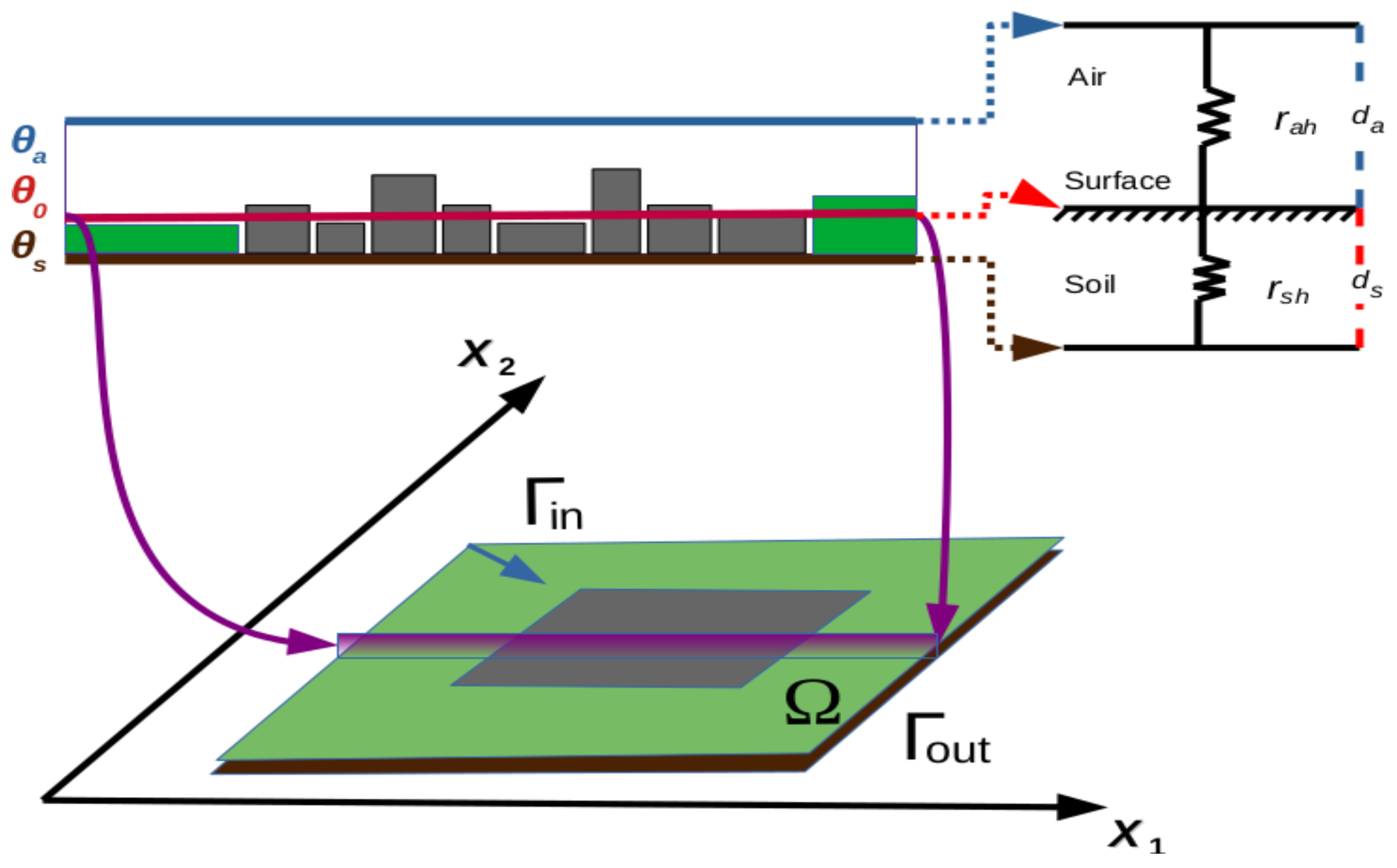
2.3. Model for Heat Transfer in Urban–Rural Domain

We are interested in simulating the temperature dynamics for our urban–rural domain. In order to achieve this objective, three temperatures are considered: air, surface, and soil, with solar radiation as their energy source. Next, air temperature is important for quantifying the UHI intensity, and it is strongly influenced by the wind flow field. The surface acts as a screen for the solar radiation, reflecting a fraction of it and absorbing its complement. As a consequence, the surface temperature can be determined. Meanwhile, soil temperature depended only on the energy interchange with the surface. Lastly, despite being defined on the 2D horizontal domain Ω , the mentioned temperatures are related by heat transfer at a much smaller vertical component.
Let θ a , θ 0 , and θ s denote the air, surface, and soil temperatures, respectively, which satisfy the following PDE system:
(7a) ϵ θ a t + u · θ a · ( μ a θ a ) = 1 d a { γ a ( θ 0 θ a ) + σ a ( θ 0 4 θ a 4 ) }   in   Ω × ( 0 , T ) , (7b) ( 1 a ) R s + ϵ s k y σ B θ a 4 ϵ 0 σ B θ 0 4 ρ a c a r a h ( θ 0 θ a ) ρ s c s r s h ( θ 0 θ s ) = λ L E   in   Ω × ( 0 , T ) , (7c) ( 1 ϵ ) θ s t · ( μ s θ s ) = 1 d s { γ s ( θ 0 θ s ) }   in   Ω × ( 0 , T ) ,
where we observe the porosity ϵ , the global total radiation R s , and those related to air, such as μ a , γ a , d a , and σ a , as the thermal diffusivity, convective interchange coefficient, air layer thickness, and radiation transfer coefficient, respectively. Parameters related to the soil are μ s , γ s , and d s which correlate to the thermal diffusivity, convective interchange coefficient, and soil layer thickness, respectively. Furthermore, those related to the air–surface–soil link are the albedo a, the sky emissivity ϵ s k y , the soil emissivity ϵ 0 , soil interchange resistance r s h , and air interchange resistance r a h . The complete list of the model parameters is found in Table A1.
For this system, we identified the following elements: Equation (7b) represents the energy balance on the surface, commonly used to estimate surface temperatures or other surface variables in remote sensing [22,23]. This equation formulates the equilibrium between total radiation Q * = ( 1 a ) R s + ϵ s k y σ B θ a 4 ϵ 0 σ B θ 0 4 , sensitive heat flux H = ρ a c a r a h ( θ 0 θ a ) , heat soil flux G 0 = ρ s c s r s h ( θ 0 θ s ) , and latent heat flux λ L E . The latter is obtained from the definition of the Bowen ratio, β = H λ L E , and the energy balance equation on the soil surface:
Q * = H + G 0 + λ L E .
Then, substituting the value H = β λ L E , we obtained a method for estimating the latent heat flux with the following relation [24,25]:
λ L E = ( 1 a ) R s + ϵ s k y σ B θ a 4 ϵ 0 σ B θ 0 4 ρ s c s r s h ( θ 0 θ s ) 1 + β ,
as long as a known value of β is available.
Remark 1.
Additional physical definitions are required to explain Equation (7b). The total radiation is the difference among the downward short-wave radiation or solar radiation ( 1 a ) R s , the long-wave radiation from the sky ϵ s k y σ B θ a 4 , and the upward long-wave radiation emitted by the soil ϵ 0 σ B θ 0 4 . The sensitive heat flux H and latent heat flux λ L E are the mechanisms by which the surface transfers much of the absorbed solar radiation to the air. The magnitude of H depends on the temperature difference and the resistance r a h while λ L E depends on the Bowen radius, which is related to evapotranspiration, predominantly by plants. Therefore, H and λ L E play the role of thermal regulators for the air layer temperature.
The Equations (7a,c) are formulated as a typical transport problem with diffusion, advection, and vertical averaged forcing, by d a and d s , respectively. Furthermore, the location on the domain of the three temperatures and its relation with the convective resistances r a h and r s h is shown and briefly explained in Figure 1.
The system is complemented with the initial conditions for air and soil temperatures θ a ( · , 0 ) = θ a 0 ( · ) and θ s ( · , 0 ) = θ s 0 ( · ) , where θ a 0 ( · ) and θ s 0 ( · ) are given functions. Regarding boundary conditions, it is assumed that heat escapes from the domain only by wind action in the case of the air temperature, so diffusion must be at zero on all borders. Whereas for the soil, it is assumed that soil temperature is equal on both sides of the boundary, implying zero diffusion. Therefore, the following homogeneous Neumann boundary conditions for both air and soil equations are imposed:
n · μ a θ a = 0 o n Γ × ( 0 , T ) ,
n · μ s θ s = 0 o n Γ × ( 0 , T ) ,
where n is the unit normal vector at each point of Γ and exterior to the domain Ω .
Remark 2.
Conditions (10a,b) have the advantage of simplifying the variational formulation of the model, and both conditions are a special case of the heat interchange condition n · μ θ = ϕ ( θ r e f θ ) , where ϕ > 0 and θ of the model are unknown and θ r e f is a given reference temperature.

2.4. Numerical Solution

Notice that the air density is constant, so the systems (3) and (7) are uncoupled, and they can be addressed independently. Moreover, the Darcy–Forchheimer–Brinkman Equation (1) has a viscous term that contributes to stability; meanwhile, the equations of the energy transfer model had the classic form of a transport equation. This indicates that a standard finite element methodology can be applied. Therefore, let us consider the Sobolev space V = H 1 ( Ω ) as our space of test functions, along with the L 2 inner product · , · to obtain the variational formulation, and the finite element functions of Lagrange P 1 type to achieve a stable numerical solutions [26,27,28].
Remark 3.
Note the mathematical analysis of the Darcy–Forchheimer–Brinkman and Darcy–Forchheimer equations in order to define the appropriate Sobolev spaces and to derive suitable variational problems has been studied in [29,30], thereby supporting the use of a finite element approach. However, due to the scope of this work, it is sufficient to use a variational approach based on the space H 1 ( Ω ) .

2.4.1. An Explicit Scheme for the Darcy–Forchheimer–Brinkman Equation: The Chorin Method

The Chorin method is now considered a classic method for solving the Navier–Stokes equations numerically [31], which is explicit in time and subsequently splits the model into three equations. The method has the advantage of being straightforward to formulate, at the expense of losing accuracy on the boundary conditions [26]. The method begins by formulating a semi-discrete problem in time. Let T denote the final simulation time, and for a given integer N, define the time step δ t = T / N and the time instants t n = n δ t , n = 0 , , N . The value u k * ( · , t n ) is denoted by u k n + 1 , and let us approximate the time derivative by using the backward Euler scheme, to obtain the following (hereafter, omitting the ‘*’ from the local velocity):
u k n + 1 u k n δ t + u n · u k n = 1 ρ P n x k ϵ ρ μ K u k n + 1 ρ · μ ϵ ( ϵ u k n ) ϵ 2 C F K u k n | u n | .
Next, let u ^ k be a first approximation to u k n + 1 , adding the zero u ^ k + u ^ k to the first term on the left hand side allows us to split the above equation as follows:
(12a) u ^ k u k n δ t = u n · u k n ϵ ρ μ K u k n + 1 ρ · μ ϵ ( ϵ u k n ) ϵ 2 C F K u k n | u n | , (12b) u k n + 1 u ^ k δ t = 1 ρ P n x k .
Furthermore, multiplying Equation (12a) by ϵ leads to:
ϵ u n + 1 u ^ δ t = ϵ ρ P n ,
By applying gradients on both sides and because u n + 1 satisfies the continuity Equation (4), the pressure equation is obtained:
1 δ t · ϵ u ^ = 1 ρ · ( ϵ P n ) ,
Next, by re-using Equation (12b), we formulate the following semi-discrete explicit problem: Given the initial state u k 0 ( · ) , for each n = 0 , 1 , , N 1 , find the tentative velocity u ^ k , the pressure P n , and update the velocity u k n + 1 by solving the following system of semi-discretized equations:
(15a) u ^ k = u k n + δ t u n · u k n ϵ ρ μ K u k n + 1 ρ · μ ϵ ( ϵ u k n ) ϵ 2 C F K u k n | u n | , (15b) 1 ρ · ( ϵ P n ) = 1 δ t · ( ϵ u ^ n ) , (15c) u k n + 1 = u ^ k δ t ρ P n x k .
The above system is uncoupled, so given u k n , k = 1 , 2 we obtain u ^ k from Equation (15a), following the pressure P n from (15b), and finally update u k n + 1 with Equation (15c).
Now we address its variational formulation, for this, multiply Equations (15a) and (15b) by test functions v , q V , integrate them by parts, and assuming that u ^ k , u k n , P n V , we can formulate
u ^ k , v = u k n , v + δ t u n · u k n , v ϵ ρ μ K u k n , v μ ρ ϵ ( ϵ u k n + u k n ϵ ) , v + n · μ ϵ ϵ u k n , v Γ ϵ 2 C F K u k n | u n | , v , 1 ρ ( ϵ P n , q n · ϵ P n , q Γ ) = 1 δ t · ϵ u ^ , q .
Note that the expansion μ ϵ ( ϵ u k n + u k n ϵ ) is due the variable porosity ϵ = ϵ ( x ) , and the inner products defined on the boundary Γ result from the integration by parts.
Regarding the Dirichlet boundary conditions (6a,b), they were imposed in a numerical level, so the natural condition n · ϵ u k n + 1 = 0 has to be applied on Γ i n Γ w . Meanwhile, to fulfill the condition on the outlet (6c), we split it into a velocity part and a pressure part, n · ϵ u k n + 1 = 0 and P n = 0 , respectively, enforcing the latter with a generalized condition n · P n = σ P n , here σ must be sufficiently large. Finally, the condition for the pressure on walls and the inlet boundary (6d) is applied.
Next, we formulate the finite element spaces associated with triangulation τ h
(16a) W h = { v C ( Ω ¯ ) : v | T P 1 , T τ h , n · ( ϵ v ) = 0 o n Γ } , (16b) M h = { q C ( Ω ¯ ) : q | T P 1 , T τ h , n · ( ϵ q ) = 0 o n Γ i n Γ w } ,
and we define the full discretized problem: Given the initial state u k 0 , k = 1 , 2 , find the vector ( u 1 n + 1 , u 2 n + 1 , P n ) W h × W h × M h that satisfies the follow explicit system for each index n = 0 , 1 , 2 , , N and for all pairs ( v , q ) W h × M h
(17a) u ^ k , v = u k n , v + δ t u n · u k n , v ϵ ρ μ K u k n , v + μ ρ ϵ ( ϵ u k n + u k n ϵ ) , v ϵ 2 C F K u k n | u n | , v , (17b) 1 ρ ( ϵ P n , q σ P n , q Γ o u t ) = 1 δ t · ϵ u ^ , q , (17c) u k n + 1 = u ^ k δ t ρ P n x k .
By introducing the nodal basis of spaces W h , M h , it is well known that problem (17) is then equivalent to solving a system of lineal equations built with the contribution matrices of each triangle element in τ h .
Remark 4.
Is important to consider that the unknown in the problem (17) is the local velocity on the REV u k * at instant t n , and not the average velocity u k n required in the model (7). Therefore, the average velocity has to be updated as follows:
u k n = ϵ u k * , n ,
for each index n = 1 , 2 , , N .

2.4.2. A Finite Element Approach and Implicit Time Schemes to Solve the Heat-Transfer Model

The model (7) has the classical form of a transport problem, so unlike the Chorin method, we follow the standard treatment of the finite element method and start by performing the spatial discretization. For this, Equation (7a,c) is multiplied by a test function v V , integraed by parts, and the boundary condition (10a,b) is applied. This leads to the variational formulation of the problem:
(19a) ϵ θ a t , v + u · θ a , v + μ a θ a , v = 1 d a { γ a ( θ 0 θ a ) + σ a ( θ 0 4 θ a 4 ) } , v , (19b) ( 1 ϵ ) θ s t , v + μ s θ s , v = 1 d s { γ s ( θ 0 θ s ) } , v .
It must be considered that the above equations, along with Equation (7b), form a non-linear system, so computing the gradients of the not-yet-defined residuals is essential for solving it.
Consider the finite element space associated with triangulation τ h :
V h = { v C ( Ω ¯ ) : v | T P 1 , T τ h , n · v = 0   on   Γ } .
Therefore, substituting V by V h , taking v V h , and replacing θ ( x , t ) by θ ( t ) w ( x ) with w V h leads to:
(21a) θ a t ϵ w , v + θ a { u · w , v + μ a w , v } = f a ( θ a , θ 0 ) , v , (21b) θ s t ( 1 ϵ ) w , v + θ s μ s w , v + 1 d s w , v = 1 d s γ s θ 0 , v ,
where f a ( θ a , θ 0 ) denotes the forcing by convection and radiation (right hand side of (19a)).
At this point, several time-marching schemes can be applied to resolve both equations. In this work, we chose a hybrid scheme with a BDF method of order 2 [26] to obtain stability at the first equation and the backward Euler for the last equation. Both schemes are implicit and then unconditionally stable. However, the nature of each equation is non-linear, non-linear algebraic, and linear, respectively. This motivated us to formulate an implicit method characterized by a time interval between the state variable of each equation and the other unknowns of the system, in order to use the available information.
Considering all of this, it is possible to formulate the complete discretized problem: Given the initial conditions θ a 0 and θ s 0 , find the solutions θ a n , θ 0 n , and θ s n for time instants n = 0 , 1 , 2 , , N , such that it satisfies the following system:
(22a) ( 3 θ a n 4 θ a n 1 + θ a n 2 ) ϵ w , v + 2 δ t θ a n { u · w , v + μ a w , v } = 2 δ t f a ( θ a n , θ 0 n 1 ) , v , (22b) ( 1 a ) R s + ϵ s k y σ B ( θ a n ) 4 ϵ 0 σ B ( θ 0 n ) 4 ρ a c a r a h ( θ 0 n θ a n ) ρ s c s r s h ( θ 0 n θ s n 1 ) = λ L E , (22c) ( θ s n θ s n 1 ) ( 1 ϵ ) w , v + θ s n δ t μ s w , v + 1 d s w , v = δ t 1 d s γ s θ 0 n + 1 , v .
The first equation requires two initial values: The first one is the initial condition, and the second one was estimated with a suitable Runge–Kutta method. In this work, we used an implicit Euler scheme.
At this stage, it is possible to compute the gradients needed to solve the non-linear Equation (22a,b). Therefore, let R a and R 0 be the residuals defined from Equations (22a,b), and let their gradients (while omitting index n) be expressed as follows:
R a θ a = 3 ϵ w , v + 2 δ t ( u · w , v + μ a w , v ) f a ( θ a , θ 0 ) θ a , v
(23a) = 3 ϵ w , v + 2 δ t ( u · w , v + μ a w , v ) ( γ a + 4 σ a ( θ a ) 3 ) , (23b) R 0 θ 0 = 4 ϵ 0 σ B ( θ 0 ) 3 ρ s c s r s h λ L E θ 0 n = β 1 + β 4 ϵ 0 σ B ( θ 0 ) 3 + ρ s c s r s h .
Similarly, by introducing the nodal basis of space V h , a non-linear system can be built with the contribution matrices defined by each term of Equation (22a,c) and vectors from the non-linear vector Equation (22b). The solution of this system produces the values of the state variables in each mesh node and each time instant.
Finally, MATLAB software was used to implement the finite element method and, particularly, its command fsolve was used to address the system of non-linear equations. This solver allowed us to supply the gradient (23a,b) and optionally evaluate its accuracy by comparing them with the solver’s gradients (estimated with central finite differences). This comparison proved to be effective, with a maximum error of order O ( 10 5 ) and O ( 10 6 ) for (23a) and (23b), respectively.

3. Numerical Results

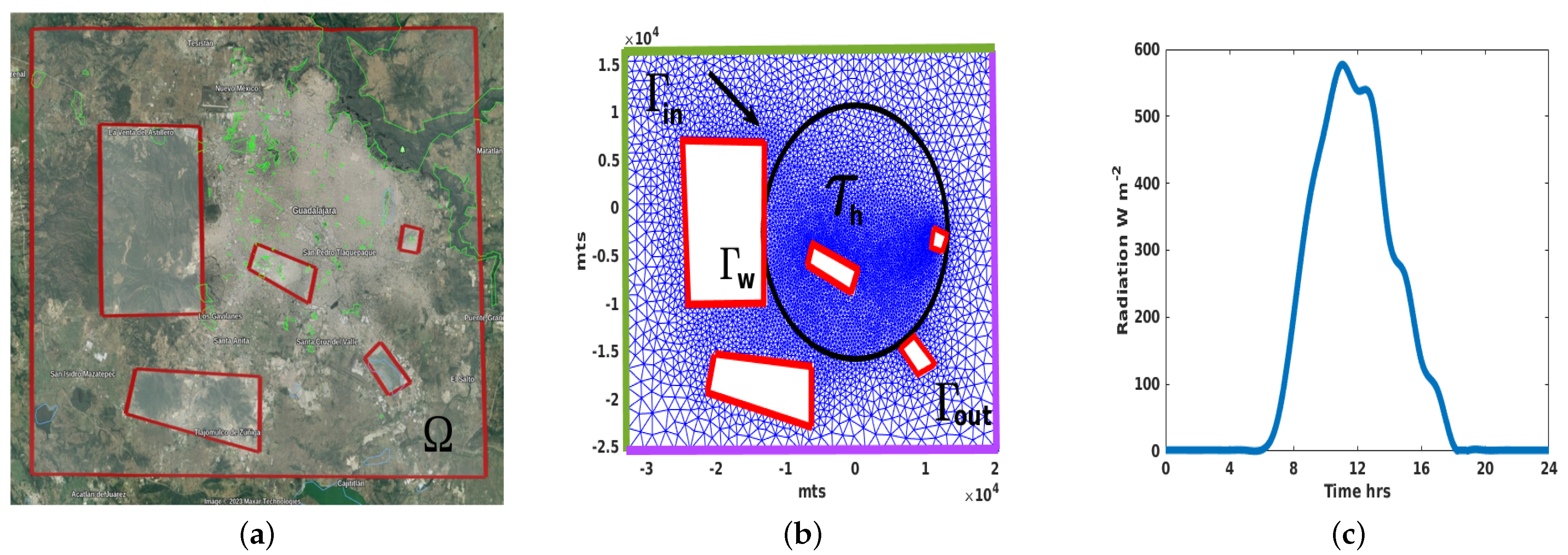
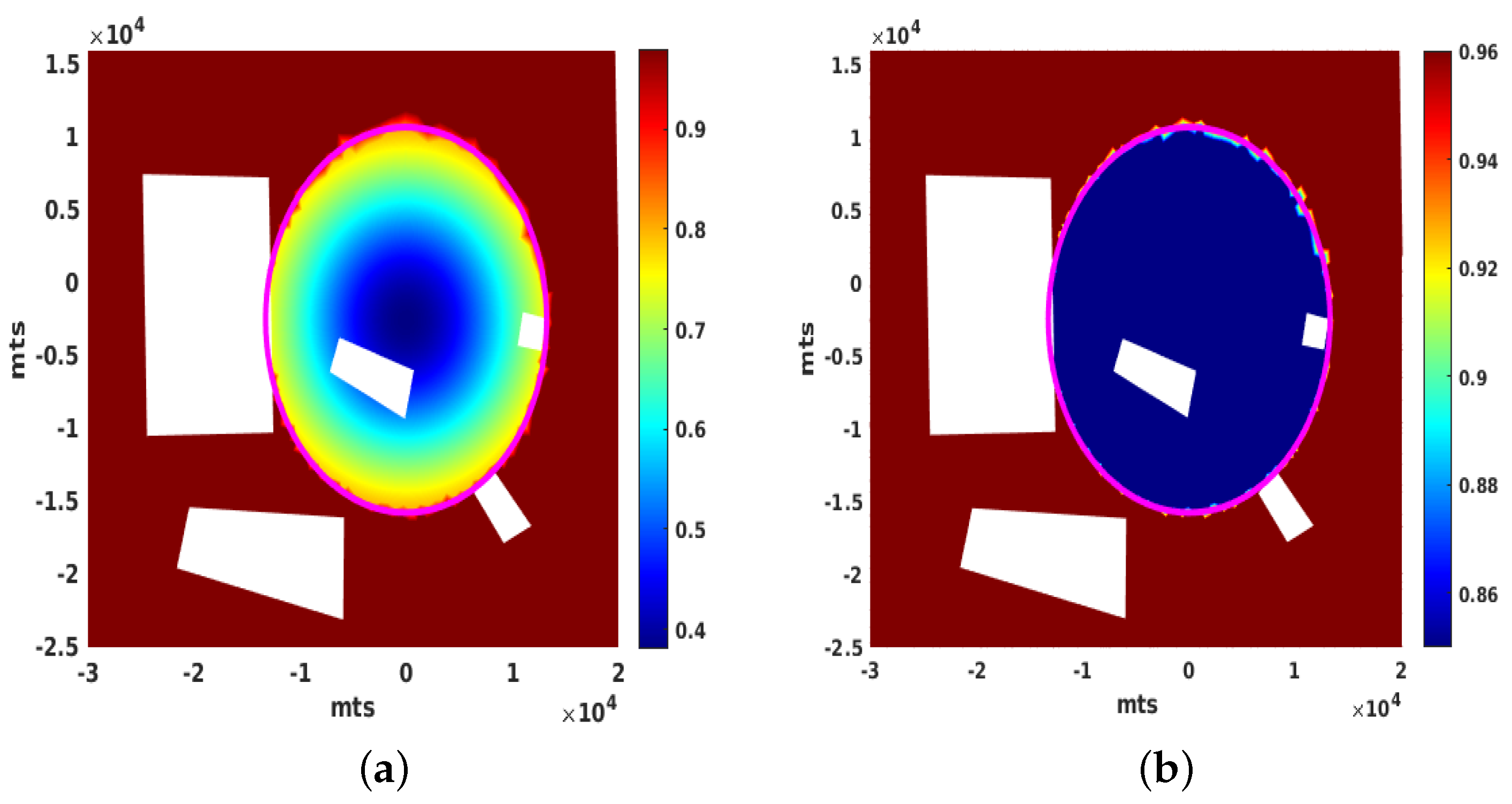
3.1. Parameters Values and the Urban–Rural Domain Based on the Metropolitan Region of Guadalajara

The domain of study considered in this work is the metropolitan region of Guadalajara in Mexico (shown in Figure 2a). Here, we observed an irregular urban boundary, along with obstacles and hills. The domain Ω was bounded by a rectangle Ω h , surrounding the hills and other small rectangles, and the constructed geometrical domain was meshed by the triangulation τ h (Figure 2b). It contained 5360 vertices and 10,338 triangular elements such that they were finer on boundary hills and urban regions in order to minimize the consequences of the no-slip boundary condition (6b) and the large temperature gradients expected in a UHI context. Moreover, we assumed that the urban–rural domain had a concentric distribution of buildings, so the center of the city presented a higher concentration of large buildings, in contrast with the suburbs, where smaller and more scattered structures were more common, and with the rural regions, where building concentration was practically nil. Therefore, the notable discrepancy on the model parameter values were intended to agree with our idealized urban–rural domain.
A key point of this work was to consider a variable porosity to characterize the urban and rural regions, instead of the use of urban–limit layouts (and without the need of boundary conditions). Therefore, given the typical porosity value [18,20] for the urban area ϵ u r b = 0.38 that is associated with high building concentrations, and for the rural area, ϵ r u r a l = 0.98 is associated with the lack of building structures. We used a simple Gaussian distribution with variances α x , α y , and centered at the city center ( x c , y c ) (see Figure 3b) to distribute them across the domain. Furthermore, in order to define the urban limits, we modeled the city as a circle with radius r, which we used to truncate the Gaussian distribution at the points where it reaches the city limits (see black and magenta lines on Figure 2b and Figure 3a). The porosity was not the only parameter related to the concentration of building blocks, as there were other factors, such as soil density ( ρ u r b = 2.11 × 10 3 , ρ r u r a l = 8.4 × 10 2 ), soil roughness ( z 0 , u r b = 7 , z 0 , r u r a l = 1 ), Bowen radius ( β u r b = 5 , β r u r a l = 0.5 ), and others that were defined with a Gaussian distribution. Nevertheless, there were dimensionless parameters, such as emissivity ( e u r b = 0.84 , e r u r a l = 0.96 ), and albedo ( a u r b = 0.27 , a r u r a l = 0.16 ), which were not dependent on the concentration of buildings. Therefore, they were defined with a radial distribution (see Figure 3b). Lastly, we used conservative values for air and soil layer thickness d a = 2 m and d s = 1 m. For a complete list of the model parameters, and the parameters associated with either urban or rural regions, see Table A1.
Remark 5.
For the sake of simplicity, we used an idealized urban–limit layout. More realistic urban layouts could be built with the curve fitting of a finite number of points on the real city limits. Nevertheless, the described methodology applies in such realistic cases.

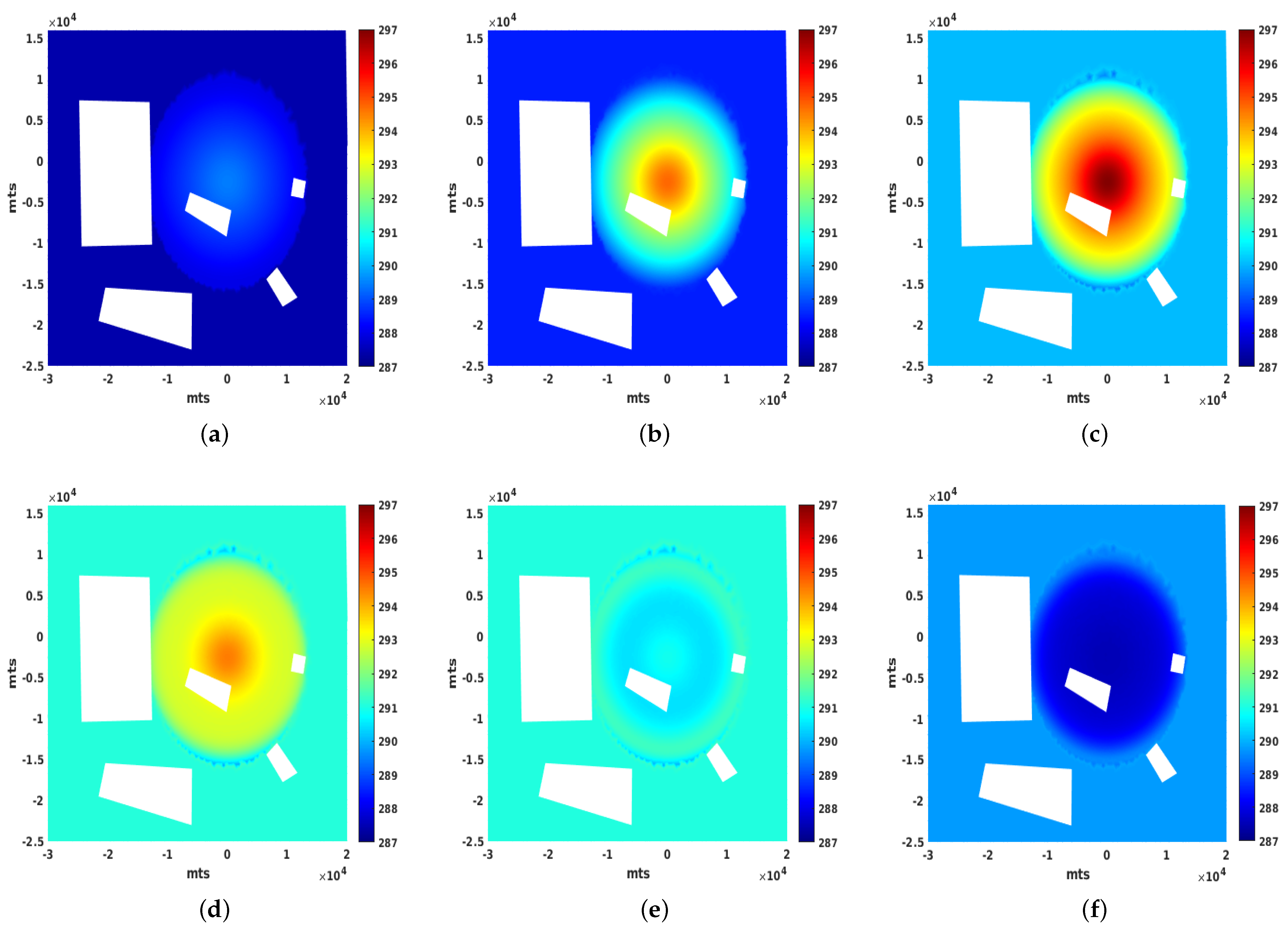
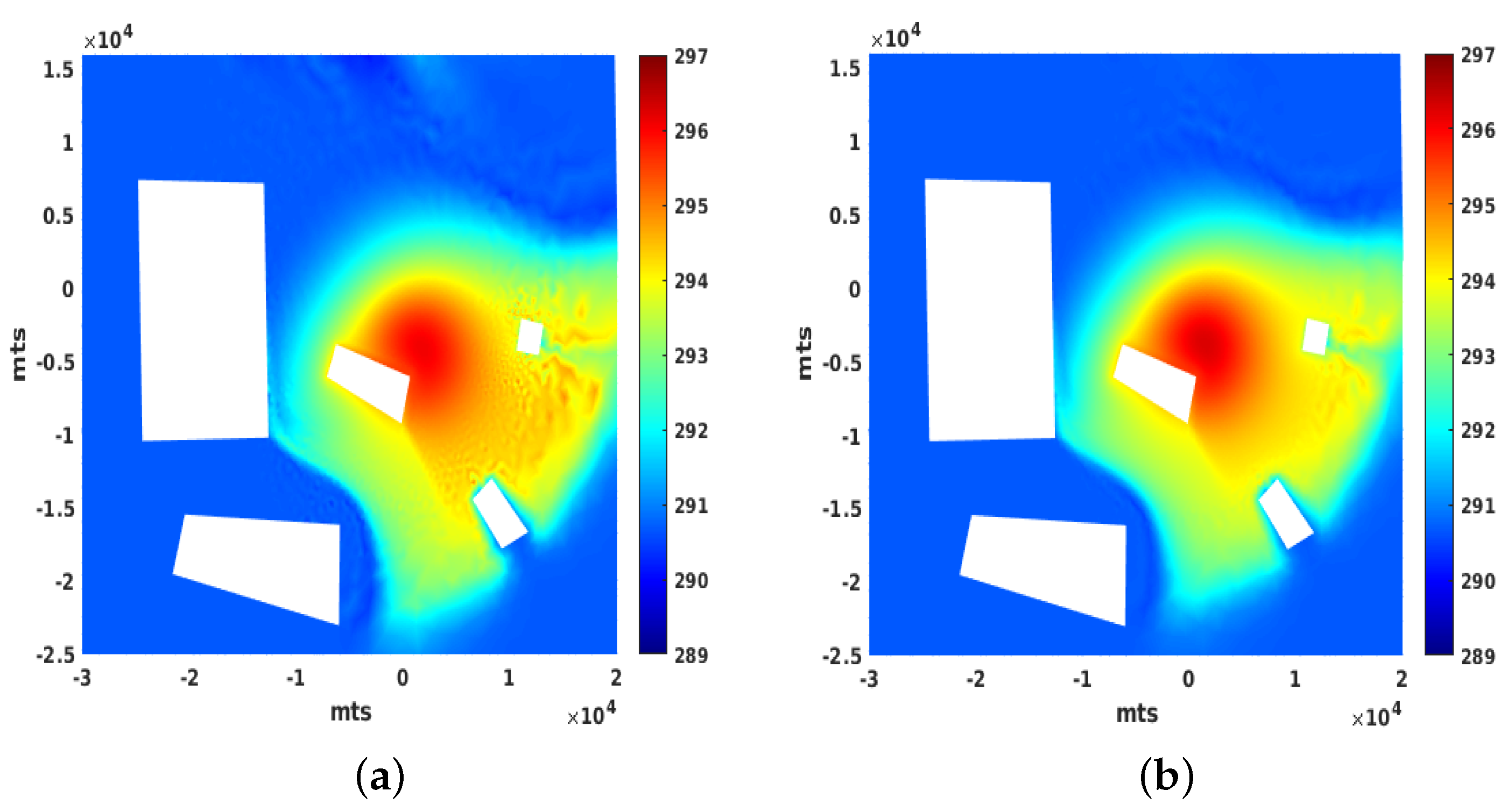
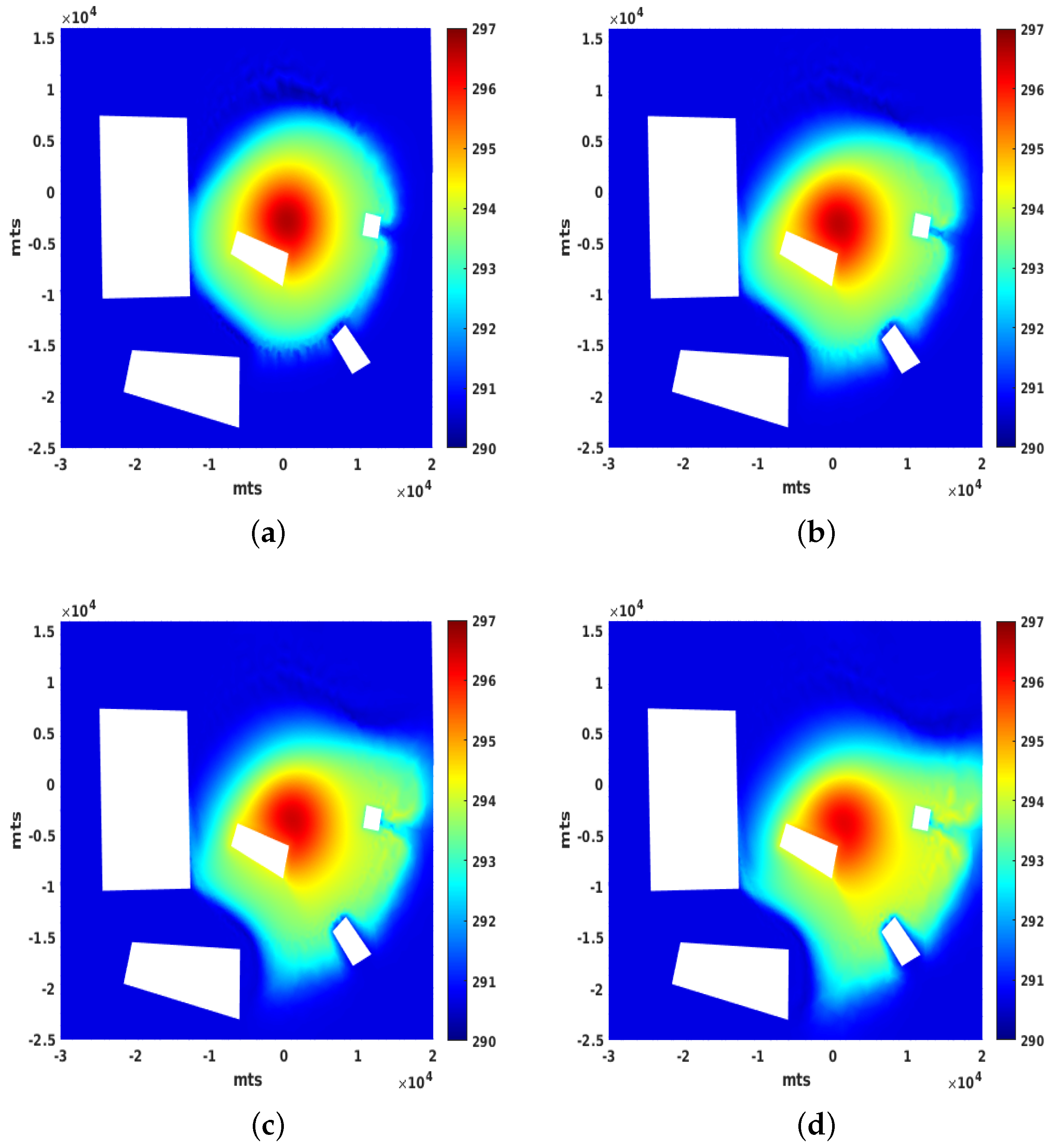
3.2. A 24 h Simulation of the UHI under Ideal Conditions

In our first test, we considered a simulation of T = 24 h under ideal conditions: no wind, a typical day-long radiation (Figure 2c), and no clouds, which was carried out with the aim of reproducing the temperature inversion described in [3,11]: a warm city during the day that transitioned into a cold city at night. Results are shown in Figure 4, where the spatial distribution of temperature θ a at 8 , 10 , 12 , 14 , 16 , 18 , and 20 h of the day is displayed. We observed not only the expected transition from a warmer urban process (consistent with radiation increase) to a colder process (consistent with radiation decrease). Both were in contrast with their rural surroundings, but they also had different heat levels, with differences of 2–3 degrees in the city (Figure 4c). This was the intended inverse temperature effect.
Remark 6.
It could be accurate to say that [11] observed the temperature inversion on parks surrounded by an urban area, that is, parks turning from a cold island during the day to a warmer island at night, with respect to their urban surroundings. Given that parks are conformed by plants, trees, and green soil, that have similar thermal properties as the rural surroundings of the city, this allowed us to assume that this phenomenon holds for a city surrounded by a rural (green) area. Therefore, the city transitioned from a heat island during the day to a cold island at night, with respect its rural surroundings.

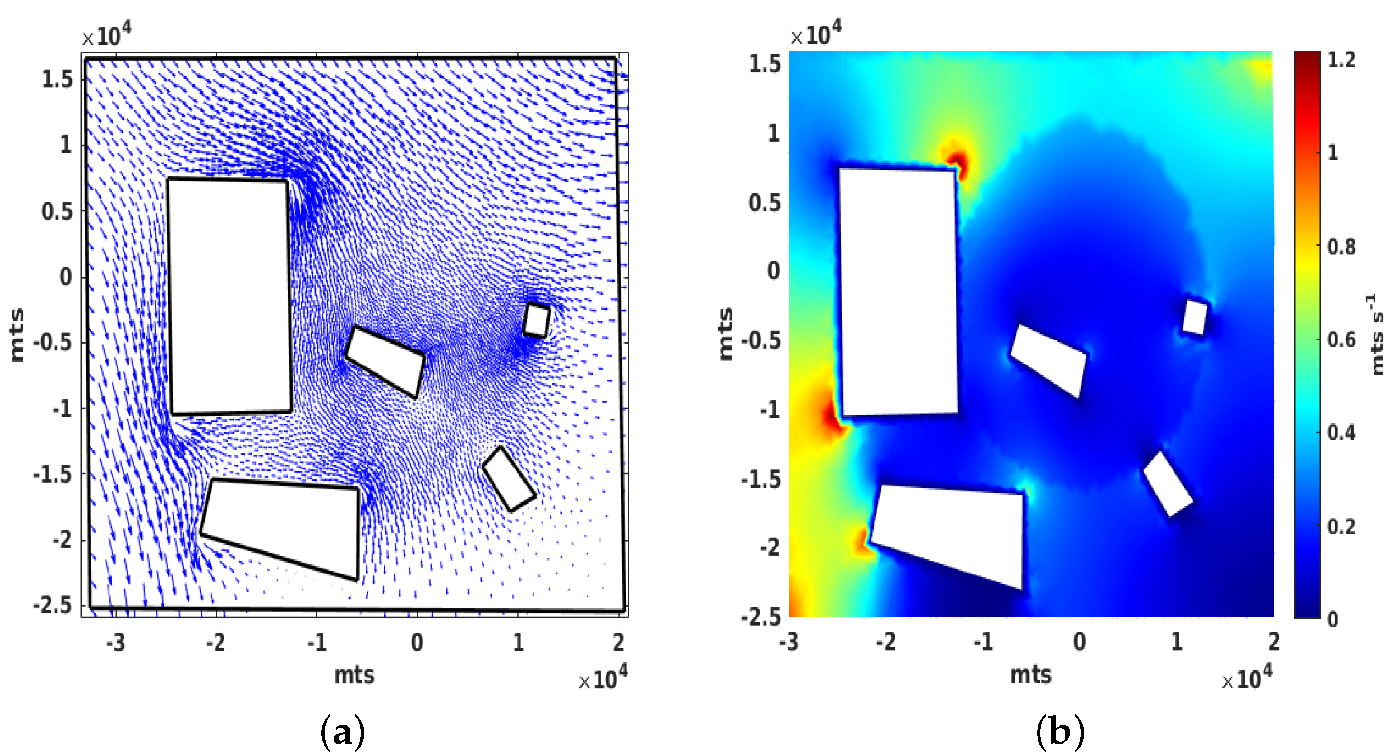
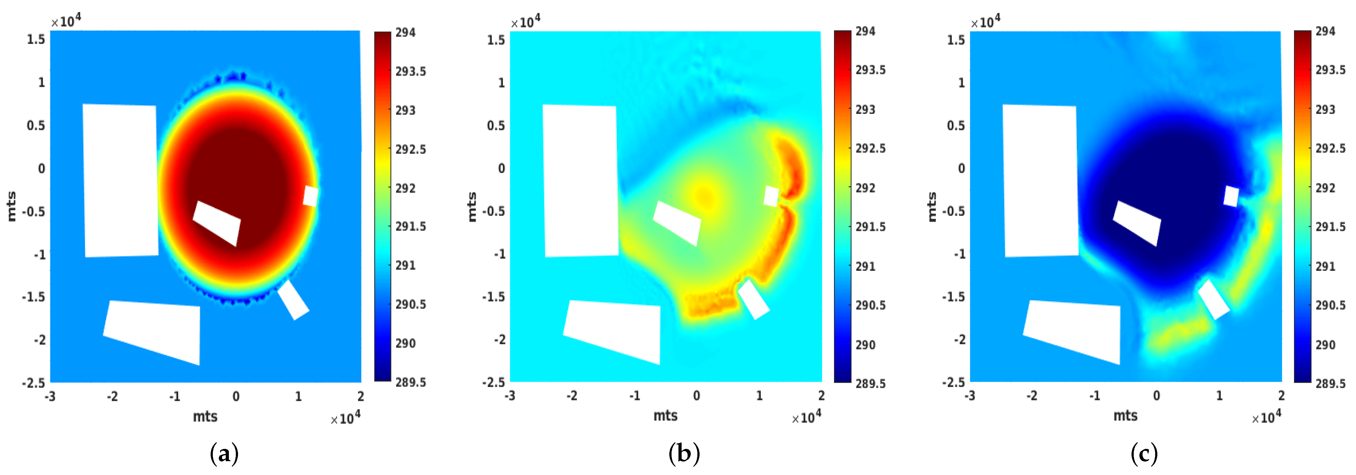
3.3. Influence of the Wind and the Need for Numerical Stabilization

With respect to the wind field, we solved the Darcy–Forchheimer–Brinkman model by forcing it with the boundary condition values g 1 = 0.25 m s 1 , and g 2 = −0.25 m s 1 , and then with an inlet wind gust in a southwest direction. Therefore, with enough time, the model achieved a stationary state which was used as the reference wind (see Figure 5), having maximum magnitude of 1.2 m s 1 . To augment the wind intensity, we used a scalar parameter η that multiplied its intensity by 1 , 2 , 3 , 4 times.
The model is highly convective due to the low density of the air and the intensity of the wind field, and this combination tends to destroy the stability of the numerical solution through spurious oscillations. This is shown in Figure 6a, where the air temperature oscillations were present along the wind direction when η = 4 and the wind blew for 3 h. To address this problem, several techniques could have been used. We chose the streamline diffusion stabilizer [28], and as shown in Figure 6b, the oscillations were minimal. The streamline diffusion stabilizer added diffusion, but only in the direction of the wind. By catching the temperature changes using an inner product between wind and θ gradient, it was implemented in the variational formulation level by adding a suitable term to Equation (19a):
ϵ θ a t , v + u · θ a , v + μ a θ a , v + ζ u · θ a , u · v = f a ( θ a , θ 0 ) , v ,
where ζ > 0 is a parameter to modulate the stabilization.
Certainly, the stabilizer is artificial, and the new variational formulation is not consistent with the strong formulation of the model, but these types of adjustments are not exclusive to the Galerkin method. For example, discontinuous Galerkin and finite volumes in heat transfer and fluid dynamics both use WENO stabilizers, which are implemented to limit the gradients between the elements of the mesh [32,33,34]. Therefore, in view of the results shown in Figure 6, future numerical experiments should use the streamline diffusion stabilizer.
Next, we analyzed the influence of different wind intensities η = 1 , 2 , 3 , 4 blowing from hour 10 to hour 13 in a day. The results are shown in Figure 7, where, as expected, the wind carried the hot mass of air to the southeast and, thereby, benefiting the northwest city inhabitants (mainly those living close to the city limits) with fresh air but disadvantaging those living in the southeast and outside of the city. The differences in the air temperatures could reach 2 K. We had to consider that radiation between the hours 10 and 13 increased, thereby continuing to heat the system. The city center did not show significant changes and maintained higher temperatures. Below, we show the changes during the afternoon.
Our last test demonstrated an interesting feature of the UHI, as it occurred when the radiation was low enough to stop the warming of the system, but at the same time, it was still subject to intense wind. The model output showed the residual mass of warmer air from the city continued to move through the countryside, exhausting its energy by interchanging it with the colder surface, until it reached the environmental temperature. At specific instants, warmer air masses had a temperature as high as 3 K higher than the rural surroundings, which was unrelated to this dynamic. For an example, see the southeast zone (Figure 8b,c). In contrast, the UHI was broken in the northwest part of the city, where the temperature contours overlapping with the city circumference boundary were no longer present. We noted that the similarities between the city circumference with temperature contours, as shown in Figure 8a, were no longer showing in the northwest section, as shown in Figure 8b, but it returned in Figure 8c with colder temperatures.

4. Discussion

In this work, a numerical study of the well-known phenomenon, urban heat island (UHI), was developed using key contributions and could be compared with other works. The characterization of the rural and urban regions using a spatially varying porosity defined by a Gaussian distribution was a different approach, with respect to the urban-monolithic type, with constant parameters or buildings distribution depending on the porosity used in the previous works ([12,16,17,18,20] and the references therein). It was interesting that the variability of the parameters enabled us to obtain a notable contrast, not only between the city and its rural surroundings, but also in the city itself, with temperature discrepancies of a few degrees. However, the porosity we defined had consequences on the model, its variational formulation, and the finite element approach, which have been explained in detail throughout the paper.
With respect to the CFD and heat-transfer models and their numerical solutions, a simple adjustment in the Darcy–Forchheimer–Brinkman equations after rewriting them with respect to the local velocity u k * , instead of the average fluid velocity u k , ensured they became classic equations of fluid dynamics with porosity-dependent forcing. Furthermore, the model for heat transfer was written based on equations used in remote sensing [23] but was adapted to the energy interchange in porous media [21]. Both allowed us to reach the proposed goals: temperature inversion and warm air transport.
From our perspective, that both models were resolved with classical numerical schemes with great accuracy was remarkable and should enable other researchers to reproduce and amplify our results. This is in contrast with more complicated methodologies, such as discontinuous finite element and finite volume methods and their limiters.
With respect to expanding our work, we inferred that our model would be able to simulate the effects of the strategies in order to mitigate the intensity of the UHI, which was evidenced in recently published reviews [15,35]: great and median urban parks [35,36], the use of white-green roofs [37], trees with dense vegetation [15,38], and the use of concrete instead of asphalt [39]. However, those strategies must be carried out in a large enough area to influence the numerical results.
Last, but not least, this paper presented challenges to be considered in future research, such as a sensitivity analysis of the influence of the model parameters on the numerical outputs; a vertical extension of the model that considers the turbulent transport; and improvements to the layout of the urban limits. Regarding the latter, there are at least two possible alternatives, using boundary conditions in an urban layout (more complicated mathematical formulation and computational effort) or defining the urban limit layout by truncating a continuous function, as we did in this work.

Author Contributions

Conceptualization, N.G.-C., J.A.L.-S., and L.G.G.-I.; methodology, N.G.-C., J.A.L.-S., and L.G.G.-I.; software, N.G.-C., J.A.L.-S., and L.G.G.-I.; investigation, N.G.-C., J.A.L.-S., and L.G.G.-I.; writing—original draft preparation, N.G.-C. and J.A.L.-S.; supervision, N.G.-C. and J.A.L.-S.; funding acquisition, N.G.-C. All authors have read and agreed to the published version of the manuscript.

Funding

This research was funded by CONACyT-Ciencia de Frontera (México) grant number 217556.

Data Availability Statement

The model code can be available on request in the first author Research Gate profile https://www.researchgate.net/profile/Nestor-Garcia-Chan, accessed on 2 February 2023.

Acknowledgments

The first author thanks CONACyT-Sistema Nacional de Investigadores (México) grant number SNI-52768, and Programa para el Desarrollo Profesional Docente (México) grant number PRODEP/103.5/16/8066. The second author thanks Programa para el Desarrollo Profesional Docente (México). The third author thanks CONACyT-Becas Nacional (México) grant number 1107627. Furthermore, the authors appreciate the comments of the anonymous reviewers that helped to improve this paper.

Conflicts of Interest

The authors declare no conflict of interest.

Appendix A

Table A1. Complete list of parameters: Value, definitions, and units [4,11,18,20].
Symbol/FormulaDefinitionValue/Units
R s Global solar radiationW m 2
ρ Fluid densitykg m 3
ρ a Air density1.1614 kg m 3
ρ u r b Urban soil density2.11 × 10 3  kg m 3
ρ r u r a l Rural soil density8.4 × 10 2  kg m 3
c a Specific heat of air1005 J kg 1  K 1
c u r b Specific heat of urban soil920 J kg 1  K 1
c r u r a l Specific heat of rural soil3600 J kg 1  K 1
c s t e a m Specific heat of steam1952 J kg 1  K 1
α a i r Air conductivity0.0263 J s 1  m 1  K 1
α u r b Urban soil conductivity0.41 J s 1  m 1  K 1
α r u r a l Rural soil conductivity1.47 J s 1  m 1  K 1
h a Air convection coefficient1 J s 1 m 2 K 1
h u r b Urban soil convection coefficient0.4 J s 1 m 2 K 1
h r u r a l Rural soil convection coefficient0.2 J s 1 m 2 K 1
a u r b Urban albedo 0.27
a r u r a l Rural albedo 0.16
e u r b Urban soil emissivity 0.96
e r u r a l Rural soil emissivity 0.85
e s k y Sky emissivity 0.77
z 0 , u r b Urban soil roughness7 m
z 0 , r u r a l Rural soil roughness1 m
u * , u r b Urban friction velocity0.2 ms 1
u * , r u r a l Rural friction velocity0.5 ms 1
β u r b Urban Bowen radius 5.0
β r u r a l Rural Bowen radius 0.5
d a = 2 Air layer thickness2.0 m
d s = 1 Soil layer thickness1.0 m
kVon Karman constant 0.4
N u Nusselt number1
σ B Stephan–Boltzmann constant5.6703 × 10 8  W  m 2 K 4
rUrban radius13,250.0 m
( x c , y c ) Urban center coordinates(0, −2500) m
dDiameter of spheres1 m
C F = 175 150 ϵ 3 ; Forchheimer coefficient
( α x , α y ) Gaussian distribution variances(10 8.25 , 10 8.15 )
K = ϵ 3 d 2 150 ( 1 ϵ ) 2 Permeability
r s h = 0.75 ρ a c s t e a m α a N u Soil resistances m 1
r a h = 1 k 2 u * l n ( 2 z 0 ) 2 Air resistances m 1
σ a = σ B e s ρ s c s Air radiation interchange coefficientm  s 1 K 3
γ a = h a c a ρ a Air convective interchange coefficientm  s 1
γ s = h s c s ρ s Soil convective interchange coefficientm s 1
μ a = α a c a ρ a Air thermal diffusivitym 2 s 1
μ s = α s ρ s c s Soil thermal diffusivitym 2 s 1

References

  1. Oke, T.R.; Johnson, G.T.; Steyn, D.G.; Watson, I.D. Simulation of surface urban heat islands under ideal conditions at night part 2: Diagnosis of causation. Bound.-Layer Meteorol. 1991, 56, 339–358. [Google Scholar] [CrossRef]
  2. Johnson, G.T.; Oke, T.R.; Lyons, T.J.; Steyn, D.G.; Watson, I.D.; Voogt, J.A. Simulation of surface urban heat islands under ideal conditions at night part 1: Theory and tests against field data. Bound.-Layer Meteorol. 1991, 56, 275–294. [Google Scholar] [CrossRef]
  3. Oke, T. Boundary Layer Climates; Taylor & Francis: Boca Raton, FL, USA, 2002. [Google Scholar]
  4. Sportisse, B. Fundamentals in Air Pollution; Springer: Dordrecht, The Netherlands, 2010. [Google Scholar] [CrossRef]
  5. Arifwidodo, S.D.; Chandrasiri, O.; Abdulharis, R.; Kubota, T. Exploring the effects of urban heat island: A case study of two cities in Thailand and Indonesia. APN Sci. Bull. 2019, 9. [Google Scholar] [CrossRef] [Green Version]
  6. Ward, K.; Lauf, S.; Kleinschmit, B.; Endlicher, W. Heat waves and urban heat islands in Europe: A review of relevant drivers. Sci. Total Environ. 2016, 569–570, 527–539. [Google Scholar] [CrossRef] [PubMed]
  7. Li, X.; Zhou, Y.; Yu, S.; Jia, G.; Li, H.; Li, W. Urban heat island impacts on building energy consumption: A review of approaches and findings. Energy 2019, 174, 407–419. [Google Scholar] [CrossRef]
  8. Cui, Y.; Xiao, S.; Giometto, M.G.; Li, Q. Effects of Urban Surface Roughness on Potential Sources of Microplastics in the Atmospheric Boundary Layer. Bound.-Layer Meteorol. 2022. [Google Scholar] [CrossRef]
  9. Ulpiani, G. On the linkage between urban heat island and urban pollution island: Three-decade literature review towards a conceptual framework. Sci. Total Environ. 2020, 751, 141727. [Google Scholar] [CrossRef]
  10. Basu, R.; Samet, J.M. Relation between Elevated Ambient Temperature and Mortality: A Review of the Epidemiologic Evidence. Epidemiol. Rev. 2002, 24, 190–202. [Google Scholar] [CrossRef]
  11. Taha, H. Urban climates and heat islands: Albedo, evapotranspiration, and anthropogenic heat. Energy Build. 1997, 25, 99–103. [Google Scholar] [CrossRef] [Green Version]
  12. Wang, H.; Peng, C.; Li, W.; Ding, C.; Ming, T.; Zhou, N. Porous media: A faster numerical simulation method applicable to real urban communities. Urban Clim. 2021, 38, 100865. [Google Scholar] [CrossRef]
  13. Mirzaei, P.A.; Haghighat, F. Approaches to study Urban Heat Island—Abilities and limitations. Build. Environ. 2010, 45, 2192–2201. [Google Scholar] [CrossRef]
  14. Mirzaei, P.A. Recent challenges in modeling of urban heat island. Sustain. Cities Soc. 2015, 19, 200–206. [Google Scholar] [CrossRef] [Green Version]
  15. Tian, L.; Li, Y.; Lu, J.; Wang, J. Review on Urban Heat Island in China: Methods, Its Impact on Buildings Energy Demand and Mitigation Strategies. Sustainability 2021, 13, 762. [Google Scholar] [CrossRef]
  16. Ming, T.; Lian, S.; Wu, Y.; Shi, T.; Peng, C.; Fang, Y.; de Richter, R.; Wong, N.H. Numerical Investigation on the Urban Heat Island Effect by Using a Porous Media Model. Energies 2021, 14, 4681. [Google Scholar] [CrossRef]
  17. Saitoh, T.; Shimada, T.; Hoshi, H. Modeling and simulation of the Tokyo urban heat island. Atmos. Environ. 1996, 30, 3431–3442. [Google Scholar] [CrossRef]
  18. Saitoh, T.S.; Yamada, N. Experimental and numerical investigation of thermal plume in urban surface layer. Exp. Therm. Fluid Sci. 2004, 28, 585–595. [Google Scholar] [CrossRef]
  19. Hang, J.; Li, Y. Wind Conditions in Idealized Building Clusters: Macroscopic Simulations Using a Porous Turbulence Model. Bound.-Layer Meteorol. 2010, 136, 129–159. [Google Scholar] [CrossRef] [Green Version]
  20. Hu, Z.; Yu, B.; Chen, Z.; Li, T.; Liu, M. Numerical investigation on the urban heat island in an entire city with an urban porous media model. Atmos. Environ. 2012, 47, 509–518. [Google Scholar] [CrossRef]
  21. Das, M.K.; Mukherjee, P.P.; Muralidhar, K. Modeling Transport Phenomena in Porous Media with Applications; Springer International Publishing: Zurich, Switwerland, 2018. [Google Scholar] [CrossRef]
  22. Bastiaanssen, W.G.M.; Hoekman, D.H.; Roebeling, R. A Methodology for the Assessment of Surface Resistance and Soil Water Storage Variability at Mesoscale Based on Remote Sensing Measurements: A Case Study with HAPEX-EFEDA Data; IAHS Special Publication, International Association of Hydrological Sciences: Wageningen, The Netherlands, 1994. [Google Scholar]
  23. Feddes, R.; Menenti, M.; Kabat, P.; Bastiaanssen, W. Is large-scale inverse modelling of unsaturated flow with areal average evaporation and surface soil moisture as estimated from remote sensing feasible? J. Hydrol. 1993, 143, 125–152. [Google Scholar] [CrossRef]
  24. Buttar, N.A.; Yongguang, H.; Shabbir, A.; Lakhiar, I.A.; Ullah, I.; Ali, A.; Aleem, M.; Yasin, M.A. Estimation of evapotranspiration using Bowen ratio method. IFAC-PapersOnLine 2018, 51, 807–810. [Google Scholar] [CrossRef]
  25. Hossein Ashktorab, W.; Pruitt, K.; Paw, U.; George, W. Energy balance determinations close to the soil surface using a micro-Bowen ratio system. Agric. For. Meteorol. 1989, 46, 259–274. [Google Scholar] [CrossRef]
  26. Larson, M.G.; Bengzon, F. The Finite Element Method: Theory, Implementation, and Applications; Springer: Berlin/Heidelberg, Germany, 2013. [Google Scholar] [CrossRef]
  27. Pan, H.; Rui, H. Mixed Element Method for Two-Dimensional Darcy–Forchheimer Model. J. Sci. Comput. 2011, 52, 563–587. [Google Scholar] [CrossRef]
  28. Gunzburger, M.D.; Bochev, P.B. Least-Squares Finite Element Methods; Springer: New York, NY, USA, 2009. [Google Scholar] [CrossRef] [Green Version]
  29. Cocquet, P.H.; Rakotobe, M.; Ramalingom, D.; Bastide, A. Error analysis for the finite element approximation of the Darcy–Brinkman–Forchheimer model for porous media with mixed boundary conditions. J. Comput. Appl. Math. 2021, 381, 113008. [Google Scholar] [CrossRef]
  30. Salas, J.J.; López, H.; Molina, B. An analysis of a mixed finite element method for a Darcy–Forchheimer model. Math. Comput. Model. 2013, 57, 2325–2338. [Google Scholar] [CrossRef]
  31. Chorin, A. Numerical solution of the navier-stokes equations. Math. Comput. 1968, 22, 745–762. [Google Scholar] [CrossRef]
  32. Cockburn, B.; Shu, C.W. Runge–Kutta Discontinuous Galerkin Methods for Convection-Dominated Problems. J. Sci. Comput. 2001, 16, 173–261. [Google Scholar] [CrossRef]
  33. Li, Q.B. Discontinuous Finite Elements in Fluid Dynamics and Heat Transfer; Springer: Berlin, Germany, 2006. [Google Scholar] [CrossRef]
  34. Zhou, T.; Li, Y.; Shu, C.W. Numerical Comparison of WENO Finite Volume and Runge–Kutta Discontinuous Galerkin Methods. J. Sci. Comput. 2001, 16, 145–171. [Google Scholar] [CrossRef]
  35. Aram, F.; Higueras García, E.; Solgi, E.; Mansournia, S. Urban green space cooling effect in cities. Heliyon 2019, 5, e01339. [Google Scholar] [CrossRef] [Green Version]
  36. Fernández, F.; Alvarez-Vázquez, L.; García-Chan, N.; Martínez, A.; Vázquez-Méndez, M. Optimal location of green zones in metropolitan areas to control the urban heat island. J. Comput. Appl. Math. 2015, 289, 412–425. [Google Scholar] [CrossRef]
  37. Besir, A.B.; Cuce, E. Green roofs and facades: A comprehensive review. Renew. Sustain. Energy Rev. 2018, 82, 915–939. [Google Scholar] [CrossRef]
  38. Villarreal-Olavarrieta, C.E.; García-Chan, N.; Vázquez-Méndez, M.E. Simulation of Heat and Water Transport on Different Tree Canopies: A Finite Element Approach. Mathematics 2021, 9, 2431. [Google Scholar] [CrossRef]
  39. Vásquez-Álvarez, P.E.; Flores-Vázquez, C.; Cobos-Torres, J.C.; Cobos-Mora, S.L. Urban Heat Island Mitigation through Planned Simulation. Sustainability 2022, 14, 8612. [Google Scholar] [CrossRef]
Figure 1. Heat-transfer model: the urban–rural domain Ω (bottom) is a sub-set of R 2 with an urban area, represented as a rectangle (gray); a rural area (green); the soil below (brown); inlet–outlet boundary segments; and inlet wind direction (blue arrow). Based on the horizontal section of the domain (magenta sector), the vertical distribution of the three temperatures θ a , θ 0 , and θ s is shown (top left) in congruence with the vertical interchange thermal resistances r a h and r s h for air and soil, respectively (top right). Both layer thicknesses, d a for air and d s for soil, are much smaller when compared with the horizontal scale. Finally, the resistance diagram (top right) is formulated based on Figure 6 in [23].
Mathematics 11 01140 g001
Figure 2. Study area idealization, mesh, and 24 h solar radiation. (a) Satellite photograph of the metropolitan region of Guadalajara with more of 40 km 2 (Google-Earth, 2023). Here, we denoted the boundaries and hills (idealized as rectangles) of the domain Ω with a red line. (b) Triangular mesh τ h , inlet boundary Γ i n (green), outlet boundary Γ o u t (magenta), hills walls Γ w (red), and the urban-limit layout (black) as a circumference of radius r. The black arrow shows the inlet wind direction. (c) Typical global day-long solar radiation R s ( t ) with maximum values at midday and almost zero on either side.
Mathematics 11 01140 g002
Figure 3. Examples of parameter distribution on the urban–rural domain and the urban–limit layout. (a) Gaussian distribution of the porosity ϵ with lower values at the city center and with higher values in the rural surroundings. (b) For dimensionless parameters such as soil emissivity e s , a simple radial distribution with only two values, corresponding to urban and rural, was assigned to each mesh node.
Mathematics 11 01140 g003
Figure 4. Time evolution of the air temperatures during a 24 h interval. We used the following times 8 , 12 , 16 , and 20 h as a sample to illustrate the obtained results. (a) θ a at 8 h. (b) θ a at 10 h. (c) θ a at 12 h. (d) θ a at 14 h. (e) θ a at 16 h. (f) θ a at 20 h.
Mathematics 11 01140 g004
Figure 5. The reference wind field used in the experiment was constant and computed from the momentum equation. (a) Wind field. (b) Norm of the wind field u .
Mathematics 11 01140 g005
Figure 6. It was clear that the streamline diffusion stabilizer minimized the spurious oscillation without notable changes in the temperatures. (a) Un-stabilized solution ( ζ = 0 ). (b) Stabilized solution ( ζ = 25 ).
Mathematics 11 01140 g006
Figure 7. Wind effect on the UHI. As expected, the wind transported the warmer air from urban to rural areas. With enough intensity, the wind could be a factor in cold downwind air temperatures. (a) Reference wind η = 1 . (b) Augmented reference wind η = 2 . (c) Augmented reference wind η = 3 . (d) Augmented reference wind η = 4 .
Mathematics 11 01140 g007
Figure 8. Dynamics of the transport of warmer mass air during wind gusts. (a) θ a before wind blows at 13 h. (b) θ a an in-between time period of blowing wind. (c) θ a final state at 17 h.
Mathematics 11 01140 g008
Disclaimer/Publisher’s Note: The statements, opinions and data contained in all publications are solely those of the individual author(s) and contributor(s) and not of MDPI and/or the editor(s). MDPI and/or the editor(s) disclaim responsibility for any injury to people or property resulting from any ideas, methods, instructions or products referred to in the content.

