Vegetation Patterns in the Hyperbolic Klausmeier Model with Secondary Seed Dispersal

Abstract

This work focuses on the dynamics of vegetation stripes in sloped semi-arid environments in the presence of secondary seed dispersal and inertial effects. To this aim, a hyperbolic generalization of the Klausmeier model that encloses the advective downhill transport of plant biomass is taken into account. Analytical investigations were performed to deduce the wave and Turing instability loci at which oscillatory and stationary vegetation patterns arise, respectively. Additional information on the possibility of predicting a null-migrating behavior was extracted with suitable approximations of the dispersion relation. Numerical simulations were also carried out to corroborate theoretical predictions and to gain more insights into the dynamics of vegetation stripes at, close to, and far from the instability threshold.

1. Introduction

Since the last century, a lot of effort has been made to describe the complex phenomena behind the formation of self-organized patterns observed in several contexts, such as physics, ecology, chemistry, biology, epidemiology, and others [1,2,3,4]. In 1952, Alan Turing proposed a mechanism through which a pattern-forming instability develops from the coupling of diffusion and kinetics as a destabilization of a stable, spatially uniform steady state [5]. In particular, Turing’s idea was successfully applied to provide a suitable description of the spatially periodic structures of vegetation biomass emerging over flat terrains or along the hill slopes of drylands [6,7,8,9,10,11,12,13,14]. In the former case, the resulting patterned configurations usually take different shapes, such as gaps, spots, hexagons, labyrinths, and others [15,16,17,18,19,20,21,22,23,24,25,26]. In the latter case, these structures are variously referred to as bands, tiger bushes, or stripes [12,13,14,27,28,29,30,31,32]. They were first observed in sub-Saharan Africa [33,34,35], but are also quite common in Australia [36,37], Mexico [38,39], and the Middle East [40,41,42].

Due to the difficulty of replicating such vegetation patterns in laboratory conditions as a result of the large spatial scale and the slow evolution of the above dynamics, much effort has been dedicated to improving mathematical models that can depict the transitions between homogeneously vegetated states and spatially periodic ones, as well as between two differently patterned states. In particular, a relevant body of literature on the modeling of vegetation patterns in sloped semi-arid environments was developed in [6,8,10,11,13,32]. Among the different frameworks, one of the easiest vegetation models was provided by Klausmeier [6]. In its original formulation, it is in the form of a parabolic reaction–diffusion–advection system for surface water and vegetation biomass, whose interaction and dispersal mechanisms give rise to an uphill migration of vegetation bands. In recent decades, despite the larger availability of experimental observations, some controversial interpretations of the effective band migration and the occurrence of stationary patterns in sloped semi-arid environments were raised [35,37]. Therefore, some generalizations of this model were proposed [10,11,13,43,44]. In particular, in the model proposed by Consolo and Valenti [13], the addition of an advection term for mimicking anisotropic seed transport due to overland flow [20,27,28,31,45] was able to provide the occurrence of stationary periodic patterns over hill slopes. Recently, in order to account for the inertial effects that were experimentally observed in vegetation response [46,47,48,49,50], this model was further generalized through a hyperbolic framework [51]. The hyperbolicity introduced there was also able to overcome the unphysical paradox of the infinite propagation speed of disturbances, which is typical of parabolic models, and generally offered a better description of transient and wave propagation phenomena [52,53,54,55,56,57,58,59,60,61,62,63]. In that paper, the focus was mainly on the role played by inertia and on the secondary seed effects on the pattern migration speed at the onset of instability. Indeed, most of the information was extracted by means of the characterization of traveling wave solutions.

With this in mind, in the present work, we aim to more deeply inspect the occurrence of oscillatory and stationary vegetation patterns not only at the bifurcation threshold, but also close to and far from it. Indeed, approximated expressions of the dispersion relation will be derived to extract additional information about the migration speed close to the onset of instability, and numerical simulations will be carried out to validate theoretical predictions.

This manuscript is organized as follows. In Section 2, the hyperbolic generalization of the Klausmeier model is briefly introduced, and a linear stability analysis is conducted in order to characterize the qualitative behavior of oscillatory and stationary patterns. In Section 3, which represents the main novelty of this paper, approximated expressions of the roots of the characteristic equations are introduced to gain a deeper understanding of the main features that characterize the emerging pattern. Here, particular emphasis on the onset of stationary patterns is also given. Concluding remarks are addressed in Section 4.

2. Materials and Methods

The theoretical investigations carried out here originate from the classical version of the Klausmeier model [6]. It is a simple, conceptual, two-compartment system for vegetation biomass $u(x,t)$ and surface water $w(x,t)$, and it is able to capture the mechanism behind vegetation pattern formation along the slopes of semi-arid environments, where x and t represent the space and time variables, respectively. In its original formulation, the flux of vegetation biomass obeys a classical gradient-like law, which mimics an isotropic dispersal of seeds, whereas surface water undergoes a passive transport dictated by downhill flow through the hillside. Note that water diffusion is neglected here, since advective transport along slopes is typically the dominant contribution.

Later, this model was generalized [13] to account for the additional phenomenon of secondary seed dispersal, namely, an advective transport of plant biomass. Indeed, along sloped terrains, seeds undergo, at first, a primary and isotropic loss from the plant to the land, and then, a secondary and anisotropic one due to their downhill overland transport. The simultaneous occurrence of multiple seed dispersal processes—consisting of mobilization, transport, and germination—was investigated in some previous works [13,20,27,28,31,45]. It was pointed out there that the strength of the seed advection speed plays a non-marginal role in the resulting vegetation pattern dynamics. In fact, despite its strength, it is just a small fraction of the water advection speed, and the migrating character (modulus and direction) of the emerging pattern is significantly affected.

Recently, motivated by the experimental evidence regarding the inertia of vegetation in the context of dryland ecology [46,47,48,49,50], a further generalization of the previous model was introduced in [51]. In particular, by following the Extended Thermodynamics theory [64,65], a hyperbolic version of the Klausmeier model was built. In this model, the flux of vegetation biomass was considered as an additional state variable that satisfied the classical principles of thermodynamics and that reduced to the classical Fick’s law in the stationary case.

In the present work, we make use of this model, which, in the 1D case, can be cast in matrix form as:

$${\mathbf{U}}_t+M{\mathbf{U}}_x=\mathbf{N}\left(\mathbf{U}\right),$$

(1)

where

$$\mathbf{U}=\left[\begin{array}{c}u\\ w\\ J\end{array}\right],M=\left[\begin{array}{ccc}-\psi & 0& 1\\ 0& -\nu & 0\\ \frac{1}{\tau }& 0& 0\end{array}\right],\mathbf{N}\left(\mathbf{U}\right)=\left[\begin{array}{c}f(u,w)\\ g(u,w)\\ -\frac{1}{\tau }J\end{array}\right]$$

(2)

with

$$f(u,w)=w{u}^2-Bu,g(u,w)=A-w-w{u}^2,$$

(3)

where A is the average annual rainfall, B is the plant loss, $\nu$ is the water advection speed, $\psi$ is the seed advection speed mimicking the secondary seed dispersal, $\tau$ is the inertial time associated with the vegetation biomass, and $J(x,t)$ is the dissipative flux associated with the plant evolution. Note that the original parabolic version of the Klausmeier model is recovered for $\psi =0$ and $\tau \to 0$. In (1), the subscripts denote partial derivatives with respect to the indicated variables.

Model (1)–(3), for $A<2B$, admits only a spatially homogeneous steady state ${\mathbf{U}}_D^{*}=\left(0,A,0\right)$, which is representative of a bare-soil ground, whereas for $A>2B$, there are two additional steady states:

$${\mathbf{U}}_L^{*}=\left(u_L,B/u_L,0\right),{\mathbf{U}}_S^{*}=\left(u_S,B/u_S,0\right)$$

(4)

where:

$$u_L=\frac{A-\sqrt{A^2-4B^2}}{2B},u_S=\frac{A+\sqrt{A^2-4B^2}}{2B},0<u_L<1<u_S$$

(5)

which are representative of spatially homogeneous vegetated regions. They coincide in the limit case for $A=2B$.

In the following analyses, according to the values reported in the literature [6,8,15,66], the rainfall and plant loss are taken in the ranges $B\in (0,2)$ and $A\in (0,3)$, respectively, whereas the water advection speed depends on the gradient slope and is generally taken as $\nu \lesssim 200$. Moreover, since only a small percentage of seeds that falls onto the land are transported downhill by water flow, it is realistic to assume $\psi \ll \nu$ [13,51]. In particular, to get more insights into the mechanisms giving rise to migrating or stationary patterns, let us now address linear stability analyses with the goal of determining the thresholds for wave and Turing instabilities, respectively.

To this aim, let us consider the hyperbolic model (1)–(3); we assume that B is the main control parameter and denote by ${\mathbf{U}}^{*}$ a spatially homogeneous positive steady state. Let us introduce a perturbation of such an equilibrium in the form $\mathbf{U}={\mathbf{U}}^{*}+\widehat{\mathbf{U}}exp\left(\omega t+ikx\right)$, with $\widehat{\mathbf{U}}$ being the vector of amplitude perturbation, k being the wavenumber, and $\omega$ being the growth factor. By substituting this into the governing system, we get the following dispersion relation:

$$\begin{array}{c}\tau {\omega }^3+\left[a_1-ik\tau \left(\nu +\psi \right)\right]{\omega }^2+\left\{a_2+ik\left[\tau \left(\nu f_u^{*}+\psi g_w^{*}\right)-\left(\nu +\psi \right)\right]\right\}\omega \\ +a_3+ik\left[\nu f_u^{*}+\psi g_w^{*}-\nu k^2\right]=0,\end{array}$$

(6)

where

$$\begin{array}{c}{a}_1=1-\tau \left(f_u^{*}+g_w^{*}\right),\hfill \\ a_2=\tau \left(f_u^{*}{g}_w^{*}-g_u^{*}{f}_w^{*}\right)-\left(f_u^{*}+g_w^{*}\right)+\left(1-\tau \nu \psi \right)k^2,\hfill \\ a_3=f_u^{*}{g}_w^{*}-g_u^{*}{f}_w^{*}-\left(g_w^{*}+\nu \psi \right)k^2\hfill \end{array}$$

(7)

and the asterisk denotes an evaluation at ${\mathbf{U}}^{*}$. To determine the occurrence of wave or Turing instabilities, it has to be checked how each steady state responds to spatially homogeneous and non-homogeneous perturbations.

The conditions under which ${\mathbf{U}}^{*}$ is stable with respect to homogeneous perturbations ($k=0$) read

$$f_u^{*}+g_w^{*}<0,f_u^{*}{g}_w^{*}-f_w^{*}{g}_u^{*}>0.$$

(8)

Therefore, in the above-mentioned realistic range of parameters, the desert state ${\mathbf{U}}_D^{*}$ and the vegetated one ${\mathbf{U}}_S^{*}$ are always stable, whereas the state ${\mathbf{U}}_L^{*}$ is unstable. Consequently, this latter state will not be further taken into account for pattern formation. By considering non-homogeneous perturbations ($k\ne 0$), it can be easily checked that ${\mathbf{U}}_D^{*}$ still continues to be locally stable. Consequently, the only state configuration that can give rise to self-organized patterns is ${\mathbf{U}}_S^{*}$.

Let us, then, analyze whether a wave instability may originate by means of a spatial disturbance about the uniform state ${\mathbf{U}}_S^{*}$. As is known, this instability is associated with the appearance of a purely imaginary root of the characteristic Equation (6) for a non-null value of the wavenumber. Moreover, the transition from the negative to the positive real part of such a root should take place through a maximum. By imposing these conditions, the locus of wave instability, which defines the critical value of the control parameter in terms of the other model coefficients, $B_w=B_w(A,\tau ,\nu ,\psi )$, can be implicitly expressed as:

$$27{\alpha }_4^2{\alpha }_1^2-{\alpha }_3^2{\alpha }_2^2+4{\alpha }_3^3{\alpha }_1+4{\alpha }_4{\alpha }_2^3-18{\alpha }_4{\alpha }_3{\alpha }_2{\alpha }_1=0$$

(9)

whereas the critical wavenumber at onset $k_w$ obeys:

$${\overline{\alpha }}_1{k}_w^6+{\overline{\alpha }}_2{k}_w^4+{\overline{\alpha }}_3{k}_w^2+{\overline{\alpha }}_4=0$$

(10)

where

$$\begin{array}{c}{\alpha }_1={\beta }_0{\beta }_1^2+{\beta }_1{\beta }_3\left[\nu \left(\tau B-1\right)-\psi \left(\tau +\tau u_S^2-1\right)\right]-{\beta }_3^2\left(1+u_S^2-\nu \psi \right),\hfill \\ {\alpha }_2=2{\beta }_0{\beta }_1{\beta }_2+\left({\beta }_1{\beta }_4+{\beta }_2{\beta }_3\right)\left[\nu \left(\tau B-1\right)-\psi \left(\tau +\tau u_S^2-1\right)\right]+\hfill \\ -2{\beta }_3{\beta }_4\left(1+u_S^2-\nu \psi \right)-{\beta }_3^{2}B\left(u_S^2-1\right),\hfill \\ {\alpha }_3={\beta }_0{\beta }_2^2+{\beta }_2{\beta }_4\left[\nu \left(\tau B-1\right)-\psi \left(\tau +\tau u_S^2-1\right)\right]-{\beta }_4^2\left(1+u_S^2-\nu \psi \right)-2B\left(u_S^2-1\right){\beta }_3{\beta }_4,\hfill \\ {\alpha }_4=-B{\beta }_4^2\left(u_S^2-1\right),\hfill \\ {\beta }_0=1-\tau \left(1+u_S^2-B\right)\hfill \\ {\beta }_1=-{\tau }^2\left(1+u_S^2-\nu \psi \right)\left[\psi B-\left(1+u_S^2\right)\right]-\nu {\beta }_0^2,\hfill \\ {\beta }_2=-{\tau }^{2}B\left(u_S^2-1\right)\left[\psi B-\left(1+u_S^2\right)\right]+{\beta }_0^2\left[\nu B-\psi \left(1+u_S^2\right)\right],\hfill \\ {\beta }_3={\beta }_0\left[\tau B-1+{\tau }^2\nu \psi \left(1+u_S^2-B\right)\right]-{\tau }^2\left[\psi B-\left(1+u_S^2\right)\right]\left\{\tau \left[\nu B-\psi \left(1+u_S^2\right)\right]-\left(\nu +\psi \right)\right\},\hfill \\ {\beta }_4={\beta }_0\left\{\tau B\left(u_S^2-1\right)-{\beta }_0\left[B\tau \left(u_S^2-1\right)-B+1+u_S^2\right]\right\}.\hfill \end{array}$$

(11)

and ${\overline{\alpha }}_i={\alpha }_i{|}_{B=B_w}(i=1,\dots ,4)$.

Moreover, the results of previous investigations [13,20,27,28,31,45,51] suggested that, at the onset, the sign of the imaginary part of the most unstable mode can be either positive or negative, denoting the (hypothetical) possibility of patterns migrating either downhill or uphill. Since the occurrence of downhill motion has been questioned in the literature, it is interesting to determine the boundary between these opposite regimes, namely, the scenario in which patterns become stationary. For this purpose, we look for null solutions of the characteristic Equation (6) and impose, again, that the transition from the negative to the positive real part occurs through a maximum. By following this strategy, it is possible to identify, for fixed values of $\nu$, $\psi$, and $\tau$, a Turing point $(B_T,A_T)$ in the parameter plane as:

$$\left\{\begin{array}{c}\nu B\left(u_S^2-1\right)+\left[\nu B-\psi \left(1+u_S^2\right)\right]\left(1+u_S^2-\nu \psi \right)=0\hfill \\ \left(1+u_S^2-\nu \psi \right)\left\{\left(1-\tau \nu \psi \right)\left[\nu B-\psi \left(1+u_S^2\right)\right]+\tau \nu B\left(u_S^2-1\right)+\nu \left(1+u_S^2-B\right)\right]+\hfill \\ +\nu \left[\nu B-\psi \left(1+u_S^2\right)\right]\left\{\tau \left[\psi \left(1+u_S^2\right)-\nu B\right]+\nu +\psi \right\}=0\end{array}\right.$$

(12)

where its associated critical wavenumber $k_T$ is given by:

$$k_T=\sqrt{\frac{\nu B_T-\psi \left(1+u_{S_T}^2\right)}{\nu }}$$

(13)

where $u_{S_T}=u_S{|}_{B=B_T,A=A_T}$.

The analysis performed here reveals that the qualitative behavior at the onset of the emerging patterns is, independently of their oscillatory or stationary nature, strongly affected by the hyperbolicity. However, due to the highly nonlinear and nontrivial nature of the above expressions, numerical investigations are required.

3. Results

In this section, we first present the results of numerical simulations with the twofold goal of corroborating our theoretical predictions and extracting quantitative information on the emerging traveling (migrating) patterns. Then, we discuss some results of analytical approximations that allow us to characterize the behavior of both migrating and stationary patterns. In all of the subsequent analyses, the water advection speed is set to $\nu =182.5$, which is in line with the values from the literature [6].

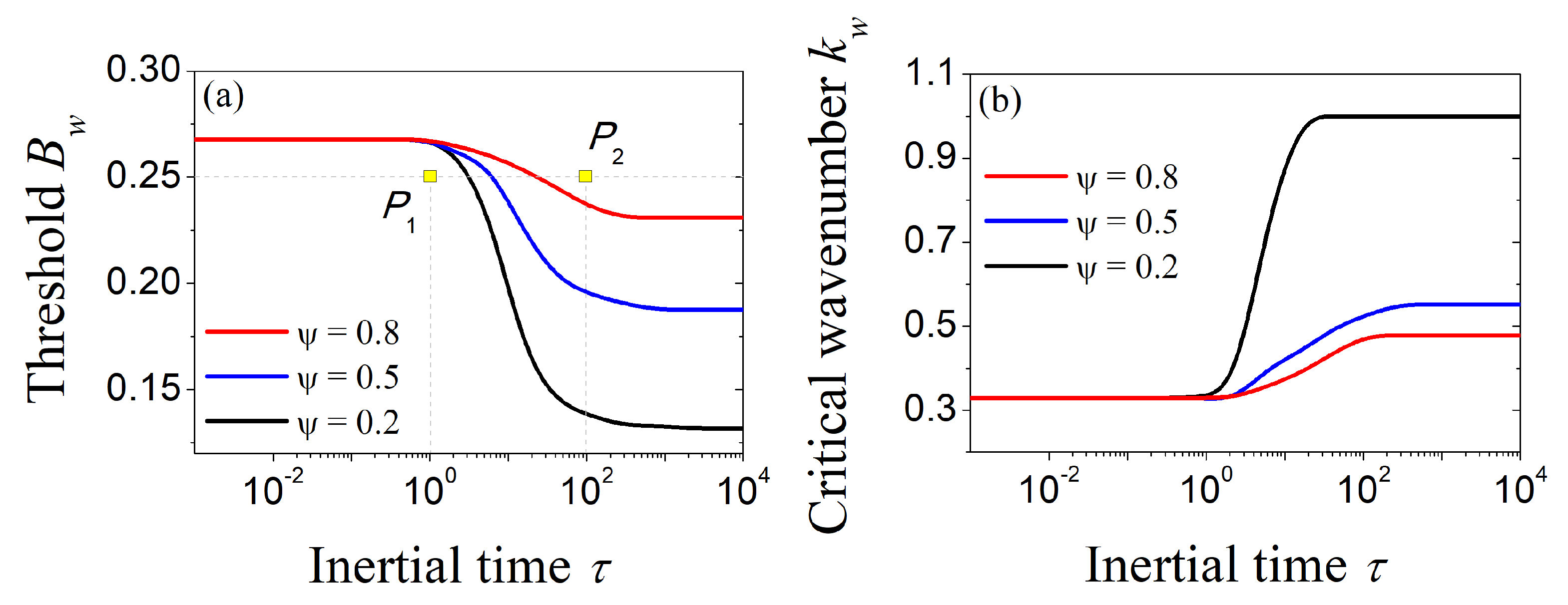
Firstly, let us numerically evaluate the dependence of the critical values of the control parameter $B_w$ and wavenumber $k_w$ at the onset of wave instability on the inertial time $\tau$ and secondary seed strength $\psi$, as theoretically predicted by (9) and (10), respectively. The results depicted in Figure 1 reveal that, close to the parabolic limit, i.e., $\tau \lesssim 1$, the critical values do not appreciably vary with $\tau$ and $\psi$. On the other hand, as we progressively move away from the parabolic limit, effects due to hyperbolicity and secondary seed dispersal become evident. Indeed, even a small increase in $\psi$ simultaneously yields a significant decrease in the critical wavenumber—thus giving rise to periodic patterns with larger wavelengths—and an increase in the critical control parameter, which implies a reduction in the pattern-forming region.

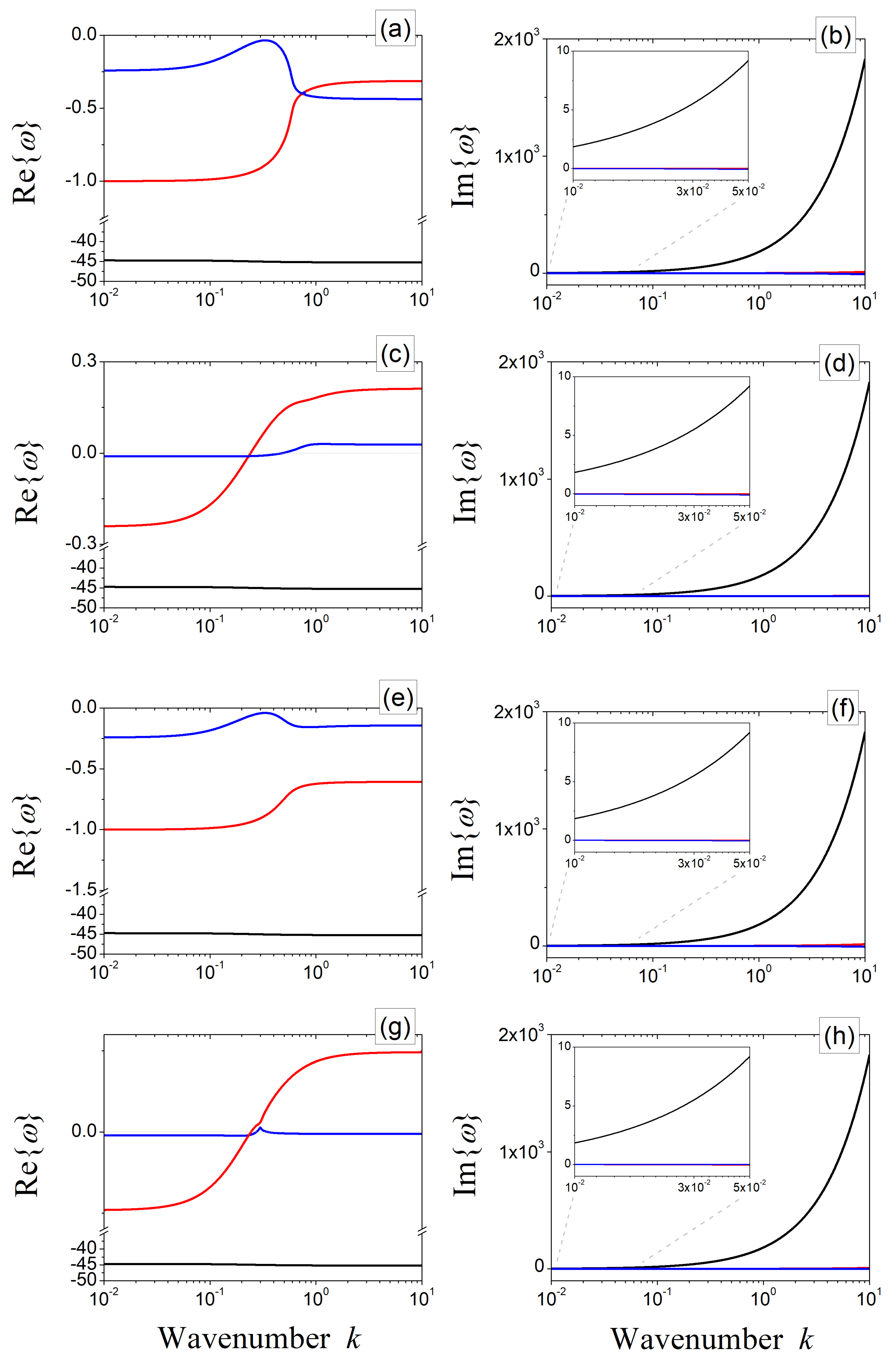
In order to gain a deeper understanding of the phenomenon of wave instability, let us track the wavenumber dependence of the roots of (6) for two points in the $(\tau ,B_w)$-plane, as reported in Figure 1a. In particular, the points P${}_1$ and P${}_2$ are chosen in such a way that they may be representative of dynamics occurring close to and far from the parabolic limit, respectively. The results are depicted in Figure 2a–d for $\psi =0.2$ and in Figure 2e–h for $\psi =0.8$. In this figure, the panels on the left (right) depict the real (imaginary) parts of the roots of the characteristic Equation (6) evaluated at P${}_1$ [panels (a),(b),(e),(f)] and P${}_2$ [panels (c),(d),(g),(h)]. As can be noticed, at the configuration P${}_1$, Equation (6) always admits roots with a negative real part (see Figure 2a,e), which is in line with the theoretical prediction reported in Figure 1a—that this point lies outside the wave bifurcation locus for all considered values of $\psi$. On the contrary, at P${}_2$, there is at least one root with a positive real part, so this point lies inside the pattern-forming region for any considered value of $\psi$ (see Figure 2c,g), which is consistent with results in Figure 1a.

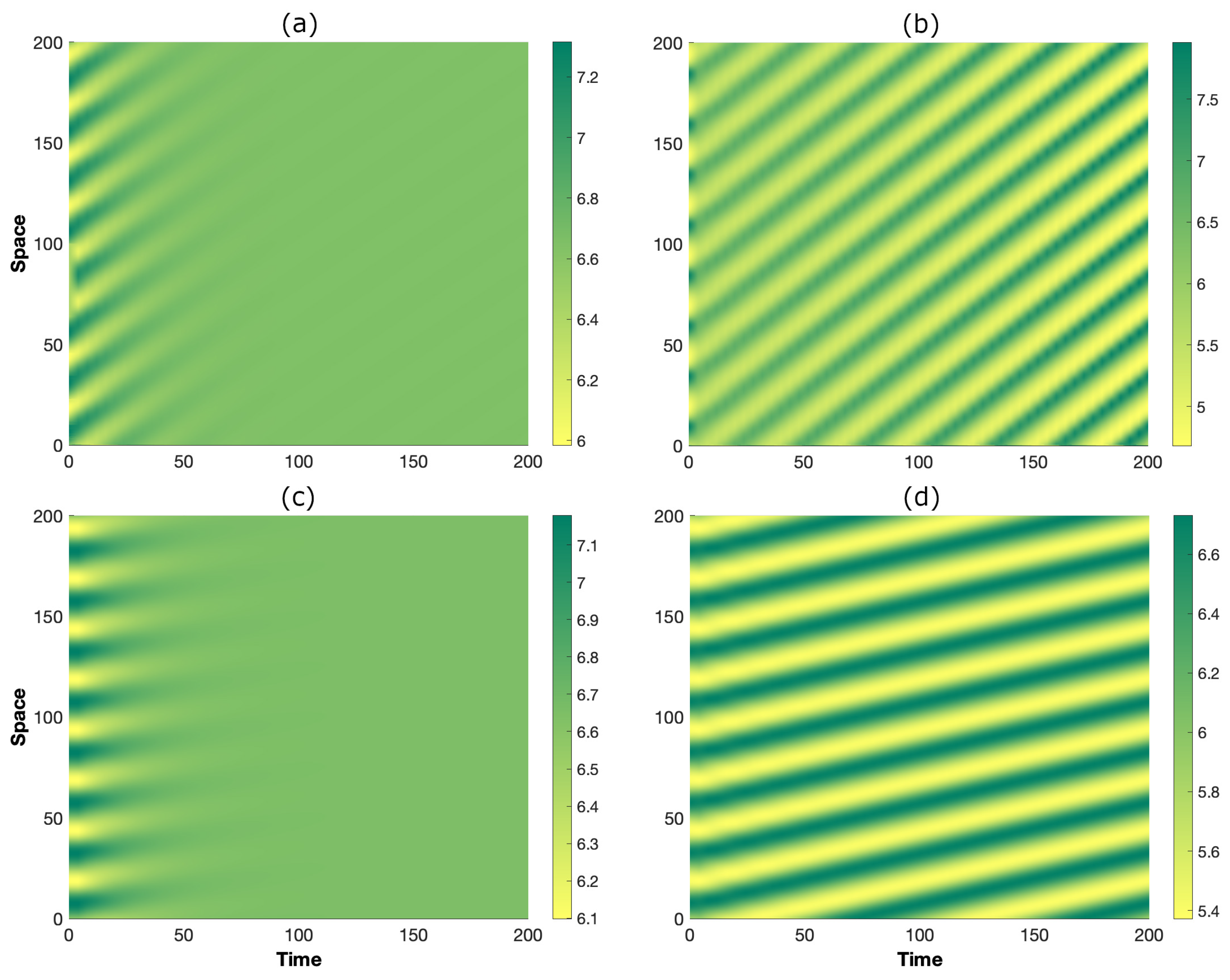
To further confirm the theoretical predictions of wave instability carried out here, system (1)–(3) is now numerically integrated by means of Matlab^® [67] in a domain $x\in [0,200]$ over a time window $t\in [0,200]$. A small perturbation around the state ${\mathbf{U}}_S^{*}$ is taken as the initial condition, and periodic boundary conditions are considered. The results are depicted in Figure 3, and they validate our previous findings. Indeed, at point P${}_1$ (panels on the left), the perturbation is absorbed, and the system relaxes towards the homogeneous steady state, whereas at point P${}_2$ (panels on the right), the spatial perturbation destabilizes the state and generates a traveling pattern. This observation highlights the role of inertia in modifying the wave bifurcation threshold. At the same time, the comparison of Figure 3b,d allows the elucidation of the role of secondary seed dispersal. In fact, as its strength is increased, the migration speed is reduced (notice the smaller slope of bands in (d) with respect to (b)) as a consequence of a larger number of seeds being transported downhill by the overland flow.

Let us now address some investigations to extract additional information from the characteristic equation. In particular, let us track the behaviors of the three complex roots of Equation (6) with the aim of identifying and determining at least an approximate expression of the functional dependence of the root responsible for the stable character of the steady state. Let us denote the roots as

$${\omega }_1=\alpha +i\beta ,{\omega }_2=\gamma +i\delta ,{\omega }_3=\theta +i\zeta ,$$

(14)

where $\alpha$, $\beta$, $\gamma$, $\delta$, $\theta$, $\zeta \in \mathbb{R}$. Then, by substituting (14) into (6) and (7), the following system in six unknowns ($\alpha$, $\beta$, $\gamma$, $\delta$, $\theta$, $\zeta$) is obtained:

$$\left\{\begin{array}{c}\alpha +\gamma +\theta =1+u_S^2-B-\frac{1}{\tau }\hfill \\ \beta +\delta +\zeta =k\left(\nu +\psi \right)\hfill \\ \theta \left(\alpha +\gamma \right)-\zeta \left(\beta +\delta \right)+\alpha \gamma -\beta \delta =\left[\tau B\left(u_S^2-1\right)+1+u_S^2-B+\left(\tau \nu \psi -1\right)k^2\right]/\tau \hfill \\ \zeta \left(\alpha +\gamma \right)+\theta \left(\beta +\delta \right)+\alpha \delta +\beta \gamma =k\left[\nu B-\psi \left(1+u_S^2\right)-\left(\nu +\psi \right)/\tau \right]\hfill \\ \theta \left(\beta \delta -\alpha \gamma \right)+\zeta \left(\alpha \delta +\beta \gamma \right)=\left[B\left(u_S^2-1\right)+\left(1+u_S^2-\nu \psi \right)k^2\right]/\tau \hfill \\ \zeta \left(\beta \delta -\alpha \gamma \right)-\theta \left(\alpha \delta +\beta \gamma \right)=k\left[\nu B-\psi \left(1+u_S^2\right)-\nu k^2\right]/\tau \hfill \end{array}\right.$$

(15)

Owing to the nontrivial structure of the above system, some simplifying assumptions are needed. One of them has an ecological foundation, i.e., $\psi \ll \nu$, as the rate at which seeds are passively transported downhill by the overland flow is quite small in comparison with the water advection speed [6,8,66]. Some others can be mathematically deduced from the inspection of the qualitative behavior of the roots reported in Figure 2. In particular, noticing that the real and imaginary parts of ${\omega }_3$ are different orders of magnitude larger than those of the other roots, it is reasonable to assume that $\zeta >>\left|\delta \right|,\left|\beta \right|$ and $\left|\theta \right|>>\left|\alpha \right|,\left|\gamma \right|$. Consequently, according to (15)${}_1$ and (15)${}_2$, the real and the imaginary part of ${\omega }_3$ can be safely approximated with Re$\left({\omega }_3\right)\approx f_u^{*}+g_w^{*}-\frac{1}{\tau }$ and Im$\left({\omega }_3\right)\approx k\nu$, respectively. Note that, according to (8), Re$\left({\omega }_3\right)$ is, thus, always negative, and, indeed, this root does not determine the stable character of ${\mathbf{U}}_S^{*}$.

By considering all of the previous assumptions, the system (15) can be approximated as

$$\begin{array}{c}\left\{\begin{array}{c}\left(1+u_S^2-B-\frac{1}{\tau }\right)\left(\alpha +\gamma \right)-k\nu \left(\beta +\delta \right)+\alpha \gamma -\beta \delta =\left[\tau B\left(u_S^2-1\right)+1+u_S^2-B+\left(\tau \nu \psi -1\right)k^2\right]/\tau \hfill \\ k\nu \left(\alpha +\gamma \right)+\left(1+u_S^2-B-\frac{1}{\tau }\right)\left(\beta +\delta \right)+\alpha \delta +\beta \gamma =k\left[\nu B-\psi \left(1+u_S^2\right)-\left(\nu +\psi \right)/\tau \right]\hfill \\ \left(1+u_S^2-B-\frac{1}{\tau }\right)\left(\beta \delta -\alpha \gamma \right)+k\nu \left(\alpha \delta +\beta \gamma \right)=\left[B\left(u_S^2-1\right)+\left(1+u_S^2-\nu \psi \right)k^2\right]/\tau \hfill \\ k\nu \left(\beta \delta -\alpha \gamma \right)-\left(1+u_S^2-B-\frac{1}{\tau }\right)\left(\alpha \delta +\beta \gamma \right)=k\left[\nu B-\psi \left(1+u_S^2\right)-\nu k^2\right]/\tau \hfill \end{array}\right.\hfill \end{array}$$

(16)

so the approximate expression for the first two roots is:

$$\begin{array}{c}{\omega }_1\approx \eta -\gamma +i\left(\frac{\theta \gamma -\chi }{\eta -2\gamma }+\theta \right),\hfill \\ {\omega }_2\approx \gamma +i\frac{\chi -\theta \gamma }{\eta -2\gamma },\hfill \end{array}$$

(17)

where $\gamma$ is implicitly defined by

$$4{\gamma }^4-8\eta {\gamma }^3+\left(5{\eta }^2+{\theta }^2-4\mu \right){\gamma }^2-\eta \left({\eta }^2+{\theta }^2-4\mu \right)\gamma +\eta \theta \chi -{\chi }^2-{\eta }^2\mu =0$$

(18)

and

$$\begin{array}{c}\eta =\frac{\left\{1-\tau \left[B-\left(1+u_S^2\right)\right]\right\}\left[B-\left(1+u_s^2\right)-\tau B\left(u_s^2-1\right)\right]+\tau {\nu }^2{k}^2\left(B-1\right)-k^2-\tau \left[B\left(u_S^2-1-k^2\right)+2k^2\left(1+u_S^2\right)\right]}{{\left\{1+\tau \left[1+u_S^2-B\right]\right\}}^2+{\tau }^2{k}^2{\nu }^2}+\hfill \\ +\frac{2{\tau }^2\nu k^2\left[\nu k^2+\psi \left(1+u_S^2\right)-\nu B\right]\left[1+\tau \left(1+u_S^2-B\right)\right]}{{\left\{{\left[1+\tau \left(1+u_S^2-B\right)\right]}^2+{\tau }^2{k}^2{\nu }^2\right\}}^2},\hfill \\ \theta =-\frac{1}{k\nu }\left\{\left(\frac{1}{\tau }+1+u_S^2-B\right)\eta +\left(\frac{1}{\tau }-\nu \psi \right)k^2+B\left(u_S^2-1\right)+\frac{1}{\tau }\left(1+u_S^2-B\right)+\right.\hfill \\ +\left.\frac{\left(B-2-u_S^2\right)\left[B\left(u_S^2-1\right)+\left(1+u_S^2+\nu \psi \right)k^2\right]+\tau \nu k^2\left[\nu B-\nu k^2-\psi \left(u_S^2+1\right)\right]}{{\left\{1+\tau \left[1+u_S^2-B\right]\right\}}^2+{\tau }^2{k}^2{\nu }^2}\right\},\hfill \\ \chi =k\frac{\left\{1-\tau \left[B-\left(1+u_S^2\right)\right]\right\}\left[\nu B-\left(1+u_s^2\right)\psi \right]-\nu k^2+\tau \nu \left[B\left(u_S^2-1\right)+\left(B-\nu \psi \right)k^2\right]}{{\left\{1+\tau \left[1+u_S^2-B\right]\right\}}^2+{\tau }^2{k}^2{\nu }^2},\hfill \\ \mu =-\frac{\left\{1-\tau \left[B-\left(1+u_S^2\right)\right]\right\}\left[B\left(u_s^2-1\right)+\left(1+u_S^2\right)k^2\right]-\nu \psi k^2+\tau {\nu }^2{k}^2\left[k^2-B\right]}{{\left\{1-\tau \left[1+u_S^2-B\right]\right\}}^2+{\tau }^2{k}^2{\nu }^2}.\hfill \end{array}$$

(19)

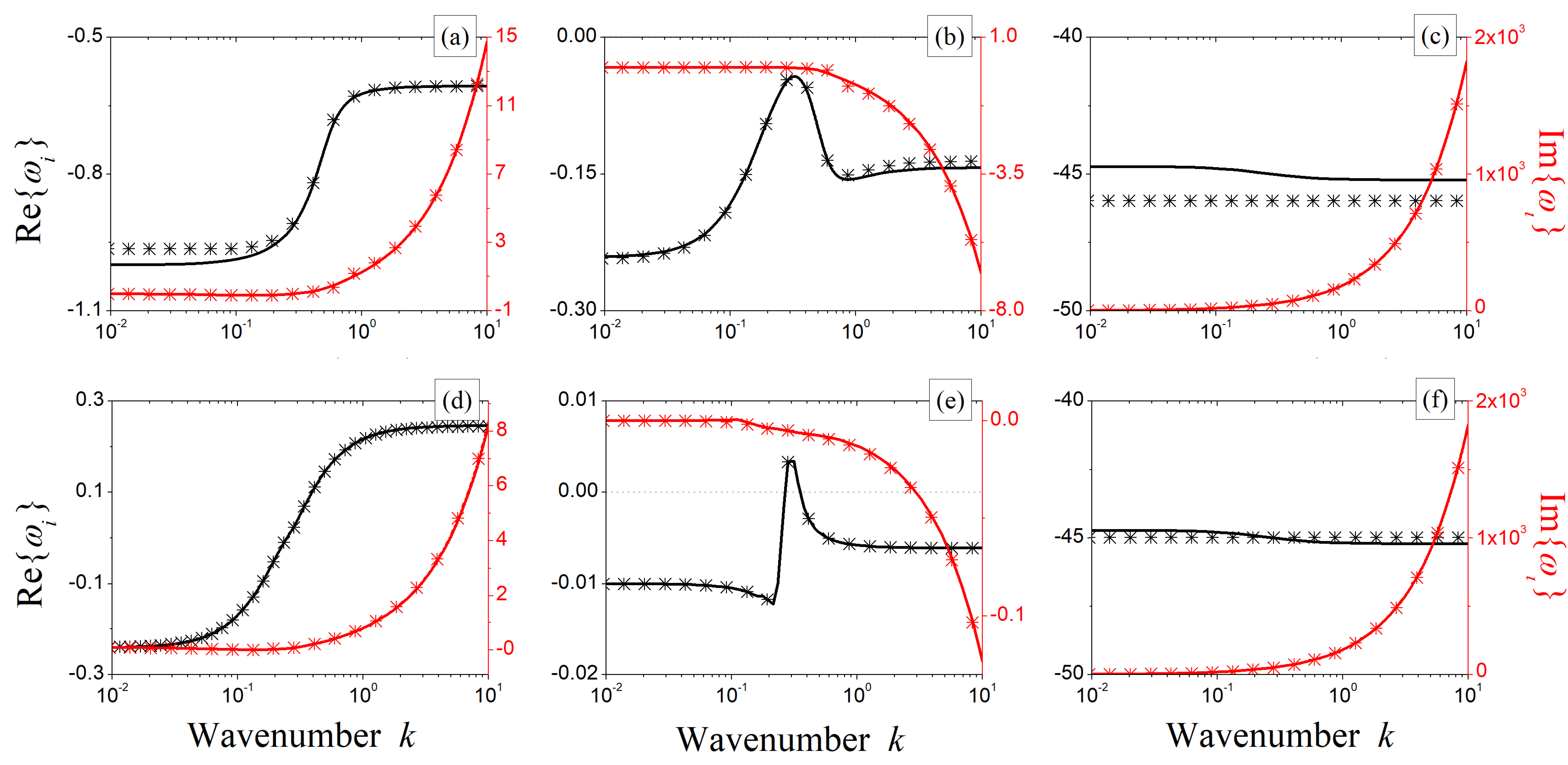
To check the validity of the approximated formulation carried out so far, in Figure 4, we present a comparison between numerically computed (solid lines) and approximated (symbols) values of the complex roots of the characteristic Equation (6). Without loss of generality, let us evaluate these roots at the points P${}_1$ and P${}_2$, which we previously introduced. Based on the satisfying agreement achieved in all cases, with a particular focus on the range of wavenumbers where the real part of the roots crosses the zero, it is possible to inspect the functional dependencies of ${\omega }_1$ and ${\omega }_2$ in more detail.

The results shown in Figure 4 also suggest that ${\omega }_1$ cannot produce any spatial instability through Turing or wave instabilities. Indeed, its real part does not cross the real axis through a maximum. Instead, it may give rise to a different kind of instability, as it originates an infinite range of unstable wavenumbers. Therefore, the only root that might be responsible for oscillatory or stationary patterns is ${\omega }_2$, whose real part exhibits the required behavior (see Figure 4b,e). For an oscillatory instability to take place, we thus need to impose the following conditions (to hold for $k\ne 0$):

$$\left\{\begin{array}{c}\mathrm{Re}\left({\omega }_2\right)=0\hfill \\ \frac{\partial \mathrm{Re}\left({\omega }_2\right)}{\partial k}=0\hfill \end{array}\right.$$

(20)

which, by virtue of (17) and (18), reduce to:

$$\left\{\begin{array}{c}\eta \theta \chi -{\chi }^2-{\eta }^2\mu =0\hfill \\ \frac{\partial }{\partial k}\left[\eta \theta \chi -{\chi }^2-{\eta }^2\mu \right]=0\hfill \end{array}\right.$$

(21)

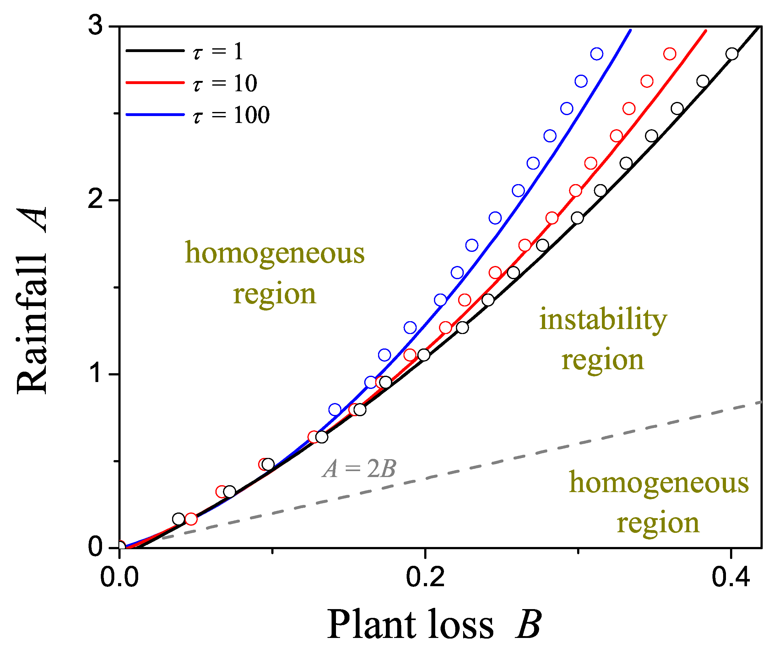
Note that Equation (21) implicitly defines the approximated critical wavenumber and the locus at which wave bifurcation occurs. Again, to check the validity of the approximated bifurcation locus, a comparison with the numerical results arising from the exact expression defined in (9) is addressed. The results shown in Figure 5 confirm a satisfactory agreement for all of the considered values of inertial times, revealing that Equation (21) may be safely used as an approximate description of key features associated with oscillatory patterns near criticality.

With this in mind, the migration speed of the oscillatory pattern at onset, under the hypothesis that the only excited mode is the one characterized by the largest growth rate, is proportional to Im$\left({\omega }_2\right)=\delta$. In particular, positive (negative) values of $\delta$ correspond to patterns migrating downhill (uphill), whereas null values are representative of stationary patterns. Therefore, taking (14) and (17) into account, the approximated locus of stationary patterns is implicitly defined by:

$$\theta \gamma -\chi =0.$$

(22)

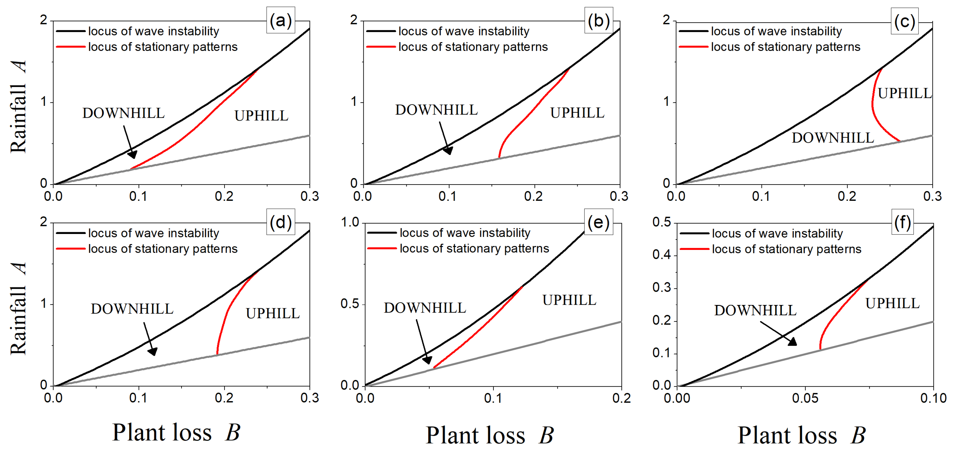
It should be noticed that such a locus exhibits a dependence on the inertial time through the coefficients $\theta$, $\gamma$, and $\chi$. Moreover, due to the implicit definition of $\gamma$, it is still necessary to rely on numerical investigations. However, the approximate expression (22) enables the possibility of evaluating the occurrence of stationary patterns in the whole parameter plane while being conscious that its validity has to be restricted to close-to-threshold values. To this aim, numerical investigations were carried out, and the results are depicted in Figure 6 for different values of inertial time $\tau$. First of all, let us focus on the behavior of stationary patterns at the onset of criticality, which corresponds to the intersection in the $(B,A)$ plane between the locus of null-migration patterns (red curve) and the wave instability one (black one). As can be noticed, for $\tau \le 1$ (panels (a)–(d)), the hyperbolicity yields a negligible effect on this intersection point, which is in reasonable agreement with our previous results (see Figure 1), thus confirming that $\tau \simeq 1$ can be considered a good approximation of the parabolic limit. When inertial effects become more relevant, the onset of stationary patterns takes place for progressively smaller values of the main control parameter (notice the different scales of the axes in panels (e)–(f)), thus enlarging the region characterized by the uphill migration of bands. Then, moving away from the wave instability threshold, the behavior of the theoretically predicted locus of stationary patterns is non-monotonous with respect to variations in inertial time. Indeed, the region of uphill migration shrinks from panel (a) to (c), whereas it is enlarged from (d) to (f). All of these results are in line with previous theoretical findings [51].

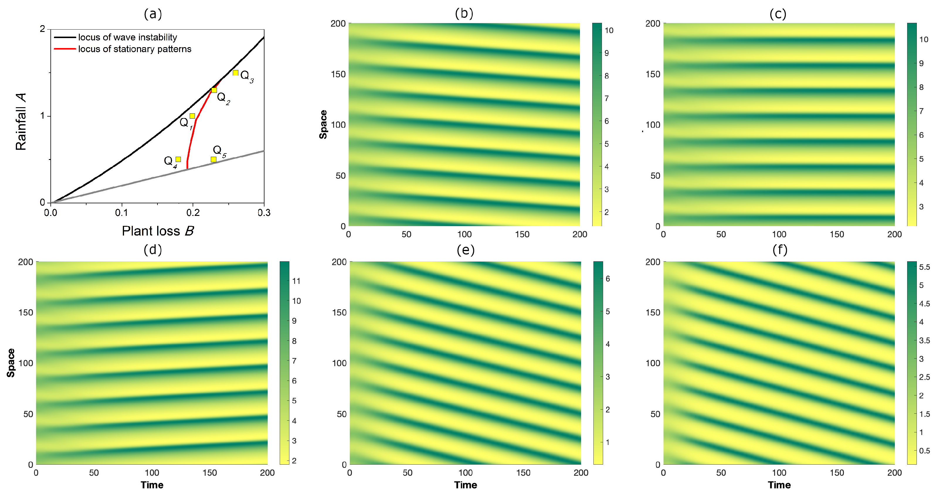
Finally, as an illustrative example of out-of-equilibrium dynamics, let us integrate the governing system (1)–(3) over $x\in [0,200]$ in a time window $t\in [0,100]$ by fixing the inertial time at $\tau =1$ and considering the configurations in the $(B,A)$ plane depicted in Figure 7a. In particular, points Q${}_1=(0.2,1)$, Q${}_2=(0.23,1.3)$, and Q${}_3=(0.25,1.5)$ correspond to near-criticality conditions, whereas Q${}_4=(0.5,0.18)$ and Q${}_5=(0.5,0.23)$ correspond to far-from-threshold ones. The overall results are shown in Figure 7b–f.

In detail, the theoretically predicted downhill, stationary, or uphill motion of bands observed near criticality at the configurations Q${}_1$, Q${}_2$, and Q${}_3$, respectively, is confirmed by our numerical simulations; see panels (b)–(d). On the contrary, in far-from-threshold conditions, the numerical results confirm the downhill motion occurring at Q${}_4$ (see panel (e)), but contradict the predictions of the uphill motion at Q${}_5$, where patterns still migrate downhill (see panel (f)). These observations provide a rough estimation of the range of validity of the approximated stationary locus. At the same time, these simulations suggest that the downhill motion of bands is the predominant behavior occurring in out-of-equilibrium conditions.

4. Conclusions

A hyperbolic generalization of the secondary seed variant of the Klausmeier model, which simultaneously accounts for secondary seed dispersal and inertial effects, was considered here to describe the migration of vegetation stripes in sloped semi-arid environments. By means of a linear stability analysis, the character of the spatially homogeneous steady states was investigated, and the conditions for the occurrence of wave and Turing instabilities were also deduced. Moreover, approximated expressions for the wavenumber dependence of the roots of the characteristic equation were derived to inspect the behavior of the emerging patterns close to the onset. These results allowed us to gain additional information on the pattern speed, locus of null-migrating patterns, and excited wavenumber.

The results attained here were corroborated by means of numerical simulations and allowed us to draw the following conclusions. First, near the parabolic limit, the behavior of stationary patterns at the onset is slightly affected by hyperbolicity. Instead, by moving away from criticality, patterns follow different migrating directions that depend on inertia. On the other hand, far from the parabolic limit, hyperbolicity favors the generation of patterns migrating uphill. Indeed, when the inertial time $\tau$ is progressively increased, the region in which downhill motion is admitted shrinks.

Finally, it is planned to extend the present study by adopting a weakly nonlinear analysis to inspect the behavior of pattern amplitude near the onset. In addition, by employing geometric singular perturbation techniques, we aim to investigate the dynamics occurring in out-of-equilibrium conditions.

References

- Murray, J.D. Mathematical Biology: I. An Introduction; Springer: New York, NY, USA, 2002. [Google Scholar]
- Murray, J.D. Mathematical Biology II: Spatial Models and Biomedical Applications; Springer: Berlin, Germany, 2003. [Google Scholar]
- Cross, M.; Greenside, H. Pattern Formation and Dynamics in Nonequilibrium Systems; Cambridge University Press: Cambridge, UK, 2009. [Google Scholar]
- Meron, E. Nonlinear Physics of Ecosystems; CRC Press: Boca Raton, FL, USA, 2015. [Google Scholar]
- Turing, A.M. The chemical basis of morphogenesis. Philos. Trans. R. Soc. Lond. 1952, 237, 37. [Google Scholar]
- Klausmeier, C.A. Regular and Irregular Patterns in Semiarid Vegetation. Science 1999, 284, 1826–1828. [Google Scholar] [CrossRef] [PubMed]
- HilleRisLambers, R.; Rietkerk, M.; van den Bosch, F.; Prins, H.H.; de Kroon, H. Vegetation pattern formation in semi-arid grazing systems. Ecology 2001, 82, 50–61. [Google Scholar] [CrossRef]
- Sherratt, J.A. An analysis of vegetation stripe formation in semi-arid landscapes. J. Math. Biol. 2005, 51, 183–197. [Google Scholar] [CrossRef] [PubMed]
- Borgogno, F.; D’Odorico, P.; Laio, F.; Ridolfi, L. Mathematical models of vegetation pattern formation in ecohydrology. Rev. Geophys. 2009, 47, RG1005. [Google Scholar] [CrossRef]
- van der Stelt, S.; Doelman, A.; Hek, G.; Rademacher, J.D. Rise and Fall of Periodic Patterns for a Generalized Klausmeier-Gray-Scott Model. J. Nonlinear Sci. 2013, 23, 39–95. [Google Scholar] [CrossRef] [Green Version]
- Siteur, K. Beyond Turing: The response of patterned ecosystems to environmental change. Ecol. Compl. 2014, 20, 81–96. [Google Scholar] [CrossRef] [Green Version]
- Marasco, A.; Iuorio, A.; Cartení, F.; Bonanomi, G.; Tartakovsky, D.M.; Mazzoleni, S.; Giannino, F. Vegetation pattern formation due to interactions between water availability and toxicity in plant-soil feedback. Bull. Math. Biol. 2014, 76, 2866–2883. [Google Scholar] [CrossRef]
- Consolo, G.; Valenti, G. Secondary seed dispersal in the Klausmeier model of vegetation for sloped semi-arid environments. Ecol. Model. 2019, 402, 66–75. [Google Scholar] [CrossRef]
- Eigentler, L.; Sherratt, J.A. An integrodifference model for vegetation patterns in semi-arid environments with seasonality. J. Math. Biol. 2020, 81, 875–904. [Google Scholar] [CrossRef]
- Rietkerk, M.; Ketner, P.; Burger, J.; Hoorens, B.; Olff, H. Multiscale soil and vegetation patchiness along a gradient of herbivore impact in a semi-arid grazing system in West Africa. Plant Ecol. 2000, 148, 207–224. [Google Scholar] [CrossRef] [Green Version]
- Von Hardenberg, J.; Meron, E.; Shachak, M.; Zarmi, Y. Diversity of vegetation patterns and desertification. Phys. Rev. Lett. 2001, 87, 198101. [Google Scholar] [CrossRef] [Green Version]
- Rietkerk, M. Self-organisation of vegetation in arid ecosystems. Am. Nat. 2002, 160, 524. [Google Scholar] [CrossRef]
- Gilad, E.; von Hardenberg, J.; Provenzale, A.; Shachak, M.; Meron, E. Ecosystem Engineers: From Pattern Formation to Habitat Creation. Phys. Rev. Lett. 2004, 93, 098105. [Google Scholar] [CrossRef]
- Thompson, S.; Katul, G.; McMahon, S.M. Role of biomass spread in vegetation pattern formation within arid ecosystems. Water Resour. Res. 2008, 44, W10421. [Google Scholar] [CrossRef]
- Thompson, S.; Katul, G. Secondary seed dispersal and its role in landscape organization. Geophys. Res. Lett. 2009, 36, L02402. [Google Scholar] [CrossRef] [Green Version]
- Deblauwe, V.; Couteron, P.; Bogaert, J.; Barbier, N. Determinants and dynamics of banded vegetation pattern migration in arid climates. Ecol. Monograph 2012, 82, 3–21. [Google Scholar] [CrossRef] [Green Version]
- Severino, G.; Giannino, F.; Cartení, F.; Mazzoleni, S.; Tartakovsky, D.M. Effects of Hydraulic Soil Properties on Vegetation Pattern Formation in Sloping Landscapes. Bull. Math. Biol. 2017, 79, 2773–2784. [Google Scholar] [CrossRef] [Green Version]
- Gandhi, P.; Werner, L.; Iams, S.; Gowda, K.; Silber, M. A topographic mechanism for arcing of dryland vegetation bands. J. R. Soc. Interface 2018, 15, 20180508. [Google Scholar] [CrossRef] [Green Version]
- Meron, E. From Patterns to Function in Living Systems: Dryland Ecosystems as a Case Study. Ann. Rev. Condens. Matt. Phys. 2018, 9, 79–103. [Google Scholar] [CrossRef]
- Gowda, K.; Iams, S.; Silber, M. Signatures of human impact on self-organized vegetation in the Horn of Africa. Sci. Rep. 2018, 8, 3622. [Google Scholar] [CrossRef] [PubMed] [Green Version]
- Marasco, A.; Giannino, F.; Iuorio, A. Modelling competitive interactions and plant-soil feedback in vegetation dynamics. Ric. Mat. 2020, 69, 553–577. [Google Scholar] [CrossRef]
- Saco, P.M.; Willgoose, G.R.; Hancock, G.R. Eco-geomorphology of banded vegetation patterns in arid and semi-arid regions. Hydrol. Earth Syst. Sci. 2007, 11, 1717–1730. [Google Scholar] [CrossRef] [Green Version]
- Ursino, N.; Rulli, M.C. Combined effect of fire and water scarcity on vegetation patterns in arid lands. Ecol. Model. 2010, 221, 2353–2362. [Google Scholar] [CrossRef]
- Sherratt, J.A.; Synodinos, A.D. Vegetation patterns and desertification waves in semi-arid environments: Mathematical models based on local facilitation in plants. Discrete Cont. Dyn. Syst. Ser. B 2012, 17, 2815–2827. [Google Scholar] [CrossRef]
- Sherratt, J.A. Pattern Solutions of the Klausmeier Model for Banded Vegetation in Semiarid Environments V: The Transition from Patterns to Desert. SIAM J. Appl. Math. 2013, 73, 1347–1367. [Google Scholar] [CrossRef]
- Thompson, S.E.; Assouline, S.; Chen, L.; Trahktenbrot, A.; Svoray, T.; Katul, G.G. Secondary dispersal driven by overland flow in drylands: Review and mechanistic model development. Mov. Ecol. 2014, 2, 4. [Google Scholar] [CrossRef] [Green Version]
- Zelnik, Y.R.; Uecker, H.; Feudel, U.; Meron, E. Desertification by front propagation? J. Theor. Biol. 2017, 418, 27–35. [Google Scholar] [CrossRef] [Green Version]
- MacFadyen, W. Vegetation patterns in the semi-desert plains of British Somaliland. Geograph. J. 1950, 115, 199–211. [Google Scholar] [CrossRef]
- Hemming, C.F. Vegetation arcs in Somaliland. J. Ecol. 1965, 53, 57–67. [Google Scholar] [CrossRef]
- Tongway, D.J. Banded Vegetation Patterning in Arid and Semiarid Environments; Springer: New York, NY, USA, 2001. [Google Scholar]
- Dunkerley, D.L.; Brown, K.J. Oblique vegetation banding in the Australian arid zone: Implications for theories of pattern evolution and maintenance. J. Arid Environ. 2002, 52, 163–181. [Google Scholar] [CrossRef]
- Dunkerley, D. Banded vegetation in some Australian semi-arid landscapes: 20 years of field observations to support the development and evaluation of numerical models of vegetation pattern evolution. Desert 2018, 23, 165–187. [Google Scholar]
- Montana, C.; Lopez-Portillo, J.; Mauchamp, A. The response of two woody species to the conditions created by a shifting ecotone in an arid ecosystem. J. Ecol. 1990, 78, 789–798. [Google Scholar] [CrossRef]
- Montaña, C. The colonisation of bare areas two-phase mosaics of an arid ecosystem. J. Ecol. 1992, 80, 315–327. [Google Scholar] [CrossRef]
- Worral, G.A. The Butanna grass pattern. J. Soil Sci. 1959, 10, 34–53. [Google Scholar] [CrossRef]
- Boaler, S.B.M.; Hodge, C.A.H. Observations on vegetation arcs in the northern region, Somali Republic. J. Ecol. 1964, 52, 511–544. [Google Scholar] [CrossRef]
- Valentin, C.; d’Herbés, J.M. Niger tiger bush as a natural water harvesting system. Catena 1999, 37, 231–256. [Google Scholar] [CrossRef]
- Kealy, B.J.; Wollkind, D.J. A nonlinear stability analysis of vegetative Turing pattern formation for an interaction–diffusion plant-surface water model system in an arid flat environment. Bull. Math. Biol. 2012, 74, 803–833. [Google Scholar] [CrossRef] [Green Version]
- Zelnik, Y.R.; Kinast, S.; Yizhaq, H.; Bel, G.; Meron, E. Regime shifts in models of dryland vegetation. Phil. Trans. R. Soc. A 2013, 321, 20120358. [Google Scholar] [CrossRef]
- Pueyo, M.; Mateu, J.; Rigol, A.; Vidal, M.; López-Sánchez, J.F.; Rauret, G. Use of the modified BCR three-step sequential extraction procedure for the study of trace element dynamics in contaminated soils. Environ. Poll. 2008, 152, 330–341. [Google Scholar] [CrossRef]
- Milchunas, D.G.; Lauenroth, W.K. Inertia in plant community structure: State changes after cessation of nutrient-enrichment stress. Ecol. Appl. 1995, 5, 452–458. [Google Scholar] [CrossRef] [Green Version]
- Garcia-Fayos, P.; Gasque, M. Consequences of a severe drought on spatial patterns of woody plants in a two-phase mosaic steppe of Stipa tenacissima. J. Arid Environ. 2002, 52, 199–208. [Google Scholar] [CrossRef]
- Deblauwe, V.; Couteron, P.; Lejeune, O.; Bogaert, J.; Barbier, N. Environmental modulation of self-organized periodic vegetation patterns in Sudan. Ecography 2011, 34, 990–1001. [Google Scholar] [CrossRef]
- Von Holle, B.; Delcourt, H.R.; Simberloff, D. The importance of biological inertia in plant community resistance to invasion. J. Veg. Sci. 2003, 14, 425–432. [Google Scholar] [CrossRef] [Green Version]
- Brown, J.H.; Whitham, T.G.; Morgan Ernest, S.K.; Gehring, C.A. Complex species interactions and the dynamics of ecological systems: Long-term experiments. Science 2001, 293, 643–650. [Google Scholar] [CrossRef] [Green Version]
- Consolo, G.; Grifó, G.; Valenti, G. Dryland vegetation pattern dynamics driven by inertial effects and secondary seed dispersal. Ecol. Model. 2022, 474, 110171. [Google Scholar] [CrossRef]
- AI-Ghoul, M.; Eu, B.C. Hyperbolic reaction-diffusion equations and irreversible thermodynamics: Cubic reversible reaction model. Phys. D 1996, 90, 119–153. [Google Scholar] [CrossRef]
- Hillen, T. Hyperbolic models for chemosensitive movement. Math. Models Methods Appl. Sci. 2002, 12, 1–28. [Google Scholar] [CrossRef]
- Mendez, V.; Fedotov, S.; Horsthemke, W. Reaction-Transport Systems; Springer: Berlin/Heidelberg, Germany, 2010. [Google Scholar]
- Straughan, B. Heat Waves; Applied Mathematical Sciences; Springer: New York, NY, USA, 2011. [Google Scholar]
- Zemskov, E.P.; Horsthemke, W. Diffusive instabilities in hyperbolic reaction-diffusion equations. Phys. Rev. E 2016, 93, 032211. [Google Scholar] [CrossRef]
- Mvogo, A.; Macías-Díaz, J.E.; Kofané, T.C. Diffusive instabilities in a hyperbolic activator-inhibitor system with superdiffusion. Phys. Rev. E 2018, 97, 032129. [Google Scholar] [CrossRef]
- Curró, C.; Valenti, G. Pattern formation in hyperbolic models with cross-diffusion: Theory and applications. Phys. D 2021, 418, 132846. [Google Scholar] [CrossRef]
- Consolo, G.; Currò, C.; Valenti, G. Pattern formation and modulation in a hyperbolic vegetation model for semiarid environments. Appl. Math. Model. 2017, 43, 372–392. [Google Scholar] [CrossRef]
- Consolo, G.; Currò, C.; Valenti, G. Supercritical and subcritical Turing pattern formation in a hyperbolic vegetation model for flat arid environments. Phys. D 2019, 398, 141–163. [Google Scholar] [CrossRef]
- Consolo, G.; Currò, C.; Valenti, G. Turing vegetation patterns in a generalized hyperbolic Klausmeier model. Math. Methods Appl. Sci. 2020, 43, 10474–10489. [Google Scholar] [CrossRef]
- Consolo, G.; Curró, C.; Grifó, G.; Valenti, G. Oscillatory periodic pattern dynamics in hyperbolic reaction-advection-diffusion models. Phys. Rev. E 2022, 105, 034206. [Google Scholar] [CrossRef]
- Consolo, G.; Grifó, G. Eckhaus instability of stationary patterns in hyperbolic reaction-diffusion models on large finite domains. Part. Diff. Eq. Appl. 2022, 3, 57. [Google Scholar] [CrossRef]
- Ruggeri, T.; Sugiyama, M. Classical and Relativistic Rational Extended Thermodynamics of Gases; Springer: Cham, Switzerland, 2021. [Google Scholar]
- Barbera, E.; Curro, C.; Valenti, G. On discontinuous travelling wave solutions for a class of hyperbolic reaction-diffusion models. Phys. D 2015, 308, 116–126. [Google Scholar] [CrossRef]
- Sherratt, J.A. Pattern solutions of the Klausmeier Model for banded vegetation in semi-arid environments I. Nonlinearity 2010, 23, 2657–2675. [Google Scholar] [CrossRef]
- MATLAB® v 9.13.0; The MathWorks Inc.: Natick, MA, USA, 2022.
Figure 1.
Inertial–time dependence of (a) the critical value of the control parameter at the onset of wave instability and (b) its associated wavenumber for different values of the seed advection speed . Fixed parameter: .
Figure 2.
Real (left panels) and imaginary (right panels) parts of the roots of the characteristic polynomial (6) as a function of the wavenumber, obtained for [panels (a–d)] and [panels (e–h)]. Panels (a,b,e,f) correspond to the point P, whereas (c,d,g,h) correspond to P. Blue, red, and black lines are representative of , , and , respectively. Fixed parameters: and .
Figure 3.
Spatio–temporal evolution obtained through the numerical integration of the governing system (1)–(3) in the configurations P [panels (a,c)] and P [panels (b,d)]. The results in the top row were obtained for [panels (a,b)], whereas those in the bottom row were obtained for [panels (c,d)]. The other parameters are as in Figure 2.
Figure 4.
Comparison between numerically computed (solid lines) and theoretically estimated (symbols) roots of the complex characteristic Equation (6) when evaluated at the points P (panels (a–c)) and P (panels (d–f)). The real parts are depicted in black, whereas the imaginary ones are depicted in red. Root is represented in panels (a,d); is depicted in (b,e), and is depicted in (c,f). Fixed parameters: , , and .
Figure 5.
The locus at which spatial bifurcations occur for different values of inertial time . Solid lines represent the numerically computed loci, whereas symbols denote the theoretically approximated predicted ones. Fixed parameters: .
Figure 6.
Loci of wave instability (black lines) and null-migration patterns (red lines) for (a) , (b) , (c) , (d) , (e) , and (f) . Fixed parameter: .
Disclaimer/Publisher’s Note: The statements, opinions and data contained in all publications are solely those of the individual author(s) and contributor(s) and not of MDPI and/or the editor(s). MDPI and/or the editor(s) disclaim responsibility for any injury to people or property resulting from any ideas, methods, instructions or products referred to in the content. |
© 2023 by the author. Licensee MDPI, Basel, Switzerland. This article is an open access article distributed under the terms and conditions of the Creative Commons Attribution (CC BY) license (https://creativecommons.org/licenses/by/4.0/).
Share and Cite
MDPI and ACS Style
Grifò, G. Vegetation Patterns in the Hyperbolic Klausmeier Model with Secondary Seed Dispersal. Mathematics 2023, 11, 1084. https://doi.org/10.3390/math11051084
AMA Style
Grifò G. Vegetation Patterns in the Hyperbolic Klausmeier Model with Secondary Seed Dispersal. Mathematics. 2023; 11(5):1084. https://doi.org/10.3390/math11051084
Chicago/Turabian StyleGrifò, Gabriele. 2023. "Vegetation Patterns in the Hyperbolic Klausmeier Model with Secondary Seed Dispersal" Mathematics 11, no. 5: 1084. https://doi.org/10.3390/math11051084
Note that from the first issue of 2016, this journal uses article numbers instead of page numbers. See further details here.