Analytical and Numerical Model of Sloshing in a Rectangular Tank Subjected to a Braking

Abstract

This paper examines the movement of waves that occur in a fuel tank—both with and without a wave breaker—when a car is travelling at a constant speed and then suddenly brakes. This phenomenon is known as slosh noise, and the paper presents an analysis of the movement of free surfaces in relation to the level of noise generated. The paper focuses on mathematical models of the fluid flow for both tanks—one without any technical solutions for breaking waves, and the other with a solution for breaking waves. The model is constructed based on a set of initial hypotheses about the fluid flow within the tank, by developing the speed potential in a series of fundamental solutions and considering the main variables that affect the phenomenon of sloshing, such as the depth of the liquid, the tank’s geometry, and the frequency and amplitude of the initial external force acting on the tank. The analysis of free surface movement is used to find the correlation with the sound generated in the tank. Nonlinearities that arise from the sudden braking are also modelled and numerically studied using MATLAB software. Following the mathematical model, a technical wave-breaking solution was implemented and tested, and it was shown that the amplitude of the movement of the free surface is reduced by half. Further research on the correspondence between the free surface movement based on the behaviour of potential energies in the two cases may be developed.

1. Introduction

Many researchers have investigated the phenomenon of sloshing using various methods: analytical [1,2], numerical or experimental. They have observed that different types of baffles, inserted in tanks [3], can reduce the natural sloshing frequencies. For example, analytical studies, numerical experiments and moving particle semi-implicit computation have been carried out using porous baffles for sloshing reduction in a swaying rectangular tank by Cho and Kim [4], and Poguluri Sunny Kumar [5], using the Galerkin method and Chebyshev polynomials for modelling and simulating the sloshing phenomenon in a porous screen-equipped tank.

It is assumed that the fuel in the tank is an incompressible fluid, and the potential formulation can be used to describe its free surface. The determination of the free surface inside the tank is closely related to the correct approximation of the sound generated by the ripple. However, the potential formulation may not always accurately express the reality [6], and numerical modelling might be necessary to produce more realistic results. The nonlinearities generated by sudden braking can also be numerically studied.

The main methods used in numerical analysis include: MAC (Marker and Cell) approximation, VOF (Volume of Fluid Method) approximation, LSM method (Level Set Method) or a combination of these methods. More recently, the SPH (Smoothed Particle Hydrodynamics) approximation [7] has been used in 2D numerical modelling to simulate sound propagation [8]. The slosh noise that occurs in a fuel tank can be a hit noise due to a wave hitting the walls of the tank, or a splash noise due to turbulence and the agglomeration of small waves inside the fuel tank. These can be studied through the oscillatory movement of the free surface of the liquid inside the fuel tank. A vertical baffle is more effective in reducing the sloshing amplitude than a horizontal one.

An improved MPS method and numerical simulation under an initial rotational excitation are made in [9], and it is proved that when the baffle is flush with the surface, the damping effect is optimal. An improved ALE technique (Arbitrary Langrangian Eulerian finite element method) was used in [10] to improve the tank design to reduce noise levels. With the same optimization goal, Frosina et al. in [11] use a CFD (Computational Fluid Dynamics) modelling approach to study the correct fuel suction under all driving conditions.

In this paper, the main variables that affect the ripple phenomenon are considered: liquid depth, tank geometry, and the frequency and amplitude of the initial external force acting on the tank. To reduce the wave nonlinearities and noise, various types of breakers can be installed in the tank. These breakers aim to reduce the pressure on the ceiling or walls, as well as to reduce extreme fluid phenomena, including ripples.

This paper is organized as follows: the problem description, general principles and hypotheses are considered in the next section. Section 3 is dedicated to the mathematical model of the fluid flow in the tank without a slosh noise reduction baffle. The fluid flow is determined by the potential of the velocity, using the method of fundamental solutions and describing the amplitude evolution of the free surface. In Section 4, the noise reduction baffle is introduced into the model. The solution of the potential function in the two areas delimited by the baffle is obtained, and the evolution of the free surface is graphically represented. The effects of using a suitable baffle are investigated. Finally, some conclusions are made.

2. Problem Description and Assumptions

We investigate the movement of waves created within a fuel tank, with and without a wave breaker, when a car is travelling at a constant speed and suddenly brakes. The aim of this study is to evaluate the effectiveness of incorporating a slosh noise buffer in a tank, both analytically and experimentally. A simplified tank shape is considered, in line with the patented technical solution for baffles proposed by the author (EP3296136A1 Dispositif Anti Clapot d’un Reservoir de Carburant d’un Vehicule Automobile, Applied By RENAULT SAS [FR], Inventor BALAS OANA MARIA [RO]).

We apply the general principles to our specific problem, taking into account boundary and initial conditions, to arrive at a well-posed problem:

$${\displaystyle \mathrm{Mass\; conservation}:{\int }_D\rho \left(\mathbf{x},t\right)dV=0,\forall D\in \mathcal{M}}$$

(1)

$${\displaystyle \mathrm{Impulse\; variation}:\frac{d}{dt}{\int }_D\rho \mathbf{a}dV={\int }_{\partial D}\mathbf{t}\mathrm{d}\sigma +{\int }_D\rho \mathbf{f}dV}$$

(2)

$${\displaystyle \mathrm{Kinetic\; moment\; variation}:\frac{d}{dt}{\int }_D\rho \mathbf{x}\times \mathbf{v}dV={\int }_{\partial D}\mathbf{x}\times \mathbf{t}\mathrm{d}\sigma +{\int }_D\mathbf{x}\times \rho \mathbf{f}\mathrm{d}V}$$

(3)

In addition to the general assumptions related to fluid motion, we add the following hypotheses:

∘

The effects of liquid compressibility, viscosity and surface tension could be neglected. According with the the first principle, we can write

$$\mathrm{div}\mathbf{v}=0.$$

(4)

∘

The flow is potential, meaning that the velocity potential $\varphi (x,y,t)$ exists such that

$${\displaystyle u=\frac{\partial \varphi }{\partial x},v=\frac{\partial \varphi }{\partial y}}$$

(5)

∘

The movement of the fluid is laminar in the z direction, and the movement is flat [12].

∘

Boundary conditions are imposed such that

$${\displaystyle \frac{d\varphi }{dn}={\mathbf{v}}_t·\mathbf{n} \mathrm{on\; the\; tank\; walls}.}$$

(6)

3. Mathematical Model of the Fluid Flow in the Tank without a Slosh Noise Reduction Baffle

The fluid flow is determined by the potential $\varphi$ of the fluid velocity that verifies the Laplace equation

$$\Delta \varphi =0$$

(7)

and boundary conditions:

$${\displaystyle \frac{\partial \varphi }{\partial x}(-l,y,t)=\frac{\partial \varphi }{\partial x}(l,y,t)=0}$$

(8)

on the side walls, and on the floor

$${\displaystyle \frac{\partial \varphi }{\partial y}(x,0,t)=0}$$

(9)

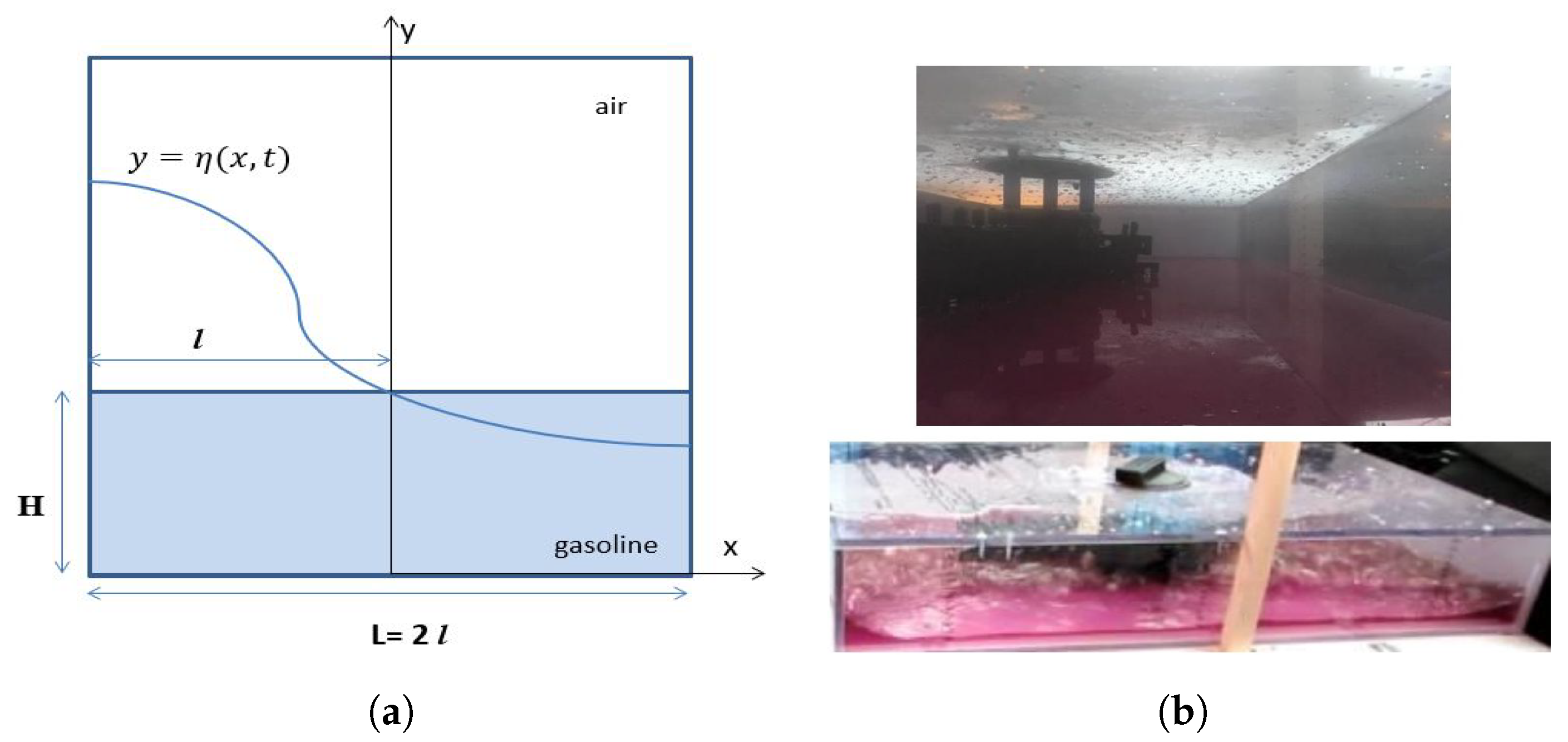
according with the geometry of the tank as in Figure 1.

The width of the tank is considered in the x direction (520 mm), the length in the z direction (1000 mm) and the height in the y direction (160 mm). The origin is considered in the middle of the bottom of the surface of the tank. Additionally, H is the height of the liquid in the tank.

The boundary condition (6) expressed for passing from the inertial coordinate system to the tank fixed coordinate system leads to the conditions imposed upon the free surface $y=\eta (x,t)$, see [13], that are the cinematic condition:

$${\displaystyle \frac{\partial \eta }{\partial t}-\mathbf{v}·\nabla \eta -\frac{\partial \eta }{\partial y}+\frac{\partial \eta }{\partial x}·\frac{\partial \varphi }{\partial x}=0}$$

(10)

and dynamic condition

$${\displaystyle \frac{\partial \varphi }{\partial t}-\mathbf{v}·\nabla \varphi +\frac{1}{2}{(\nabla \varphi )}^2+g\eta =0.}$$

(11)

As the liquid is incompressible, the potential energy of a liquid element is given only by the potential gravitational energy [3,14,15,16]:

$${\displaystyle U^e=\frac{1}{2}\rho gb{\int }_0^L{\eta }^2(x,t)\mathrm{d}x}$$

(12)

and the kinetic energy of the liquid element is given by [3,16]:

$${\displaystyle T^e=\frac{1}{2}\rho g{\int }_V{(\nabla \varphi )}^2\mathrm{d}V.}$$

(13)

When the tank is subjected to a horizontal acceleration, ${\ddot{\mathrm{X}}}_0\left(t\right)$ lateral sounds of the contained fluid will appear, where:

$${\dot{\mathrm{X}}}_0\left(t\right)=\left\{\begin{array}{cc}{U}_0-at,\hfill & t\in [0,t_1]\hfill \\ -a{t}_1,\hfill & t\in [t_1,t_s]\hfill \end{array}\right.$$

(14)

$t_s$ is the total stop time of the tank ($t_s=5\mathrm{s}$), $t_1=0.4\mathrm{s}$, $a=U_0/t_1$, and constant a represents the average value of the acceleration (of braking, in this case). Based on the state of the art of the topic developed by the authors, the optimal timing for the braking event that generates the slosh noise phenomena is 5 s. This duration it is used for the analytical model and experimental tests [17,18,19,20,21,22].

Movement in the tank is described by the potential $\varphi$ that is decomposed into two functions:

$$\varphi =\phi +\psi ,$$

(15)

where $\phi$ is the solution of the Laplace’s equation with static conditions on the walls:

$$\phi =xu+yv,$$

(16)

and $\psi$ also satisfies the Laplace’s equation in D and the following boundary conditions:

$${\displaystyle \mathrm{on\; the\; side\; walls}:\frac{\partial \psi }{\partial x}(-\frac{L}{2},y,t)=0=\frac{\partial \psi }{\partial x}(\frac{L}{2},y,t)}$$

(17)

$${\displaystyle \mathrm{on\; the\; floor\; of\; the\; tank}:\frac{\partial \psi }{\partial y}{|}_{y=0}=0}$$

(18)

$${\displaystyle \mathrm{on\; the\; free\; surface}:\frac{\partial \eta }{\partial t}-\frac{\partial \psi }{\partial y}+\frac{\partial \eta }{\partial x}·\frac{\partial \varphi }{\partial x}=0}$$

(19)

Analytical Model (Ma) for Determining the Potential

The potential will be determined using the superposition method of the liquid’s own functions in the tank, based on the linearized theory of potentials, compared to the nonlinear Boussinesq model [12].

We use the method of fundamental solutions (MFS), also described in [12,13], and consider that the potential has the form

$${\displaystyle \psi (x,y,t)={\psi }_0(x,y,t)+\sum _n{\psi }_n(x,y,t)}$$

(20)

where

$${\psi }_n(x,y,t)=f_n(x,y)A_n\left(t\right),n\ge 1$$

(21)

are the fundamental solutions that verify the Laplace equation, $\Delta \psi =0$ with the conditions (17)–(19). One finds, for the functions $f_n$, the problem

$${\displaystyle \Delta f_n=0,\frac{\partial f_n}{\partial x}\left(-\frac{L}{2},y\right)=0=\frac{\partial f_n}{\partial x}(\frac{L}{2},y),\frac{\partial f_n}{\partial y}{|}_{y=0}=0}$$

(22)

with the boundary conditions (considered linear, in the first approximation)

$${\displaystyle \frac{\partial \eta }{\partial t}-\frac{\partial \psi }{\partial y}=0,\frac{\partial \psi }{\partial t}+g\eta =0}$$

(23)

and where the first potential ${\psi }_0$ is a particular solution that takes into account the movement of the tank, verifies the Laplace equation and non-homogeneous boundary conditions

$${\displaystyle \Delta {\psi }_0=0,\frac{\partial {\psi }_0}{\partial x}(-\frac{L}{2},y,t)=\dot{X}\left(t\right)=\frac{\partial {\psi }_0}{\partial x}(\frac{L}{2},y,t),\frac{\partial {\psi }_0}{\partial y}{|}_{y=0}=0.}$$

(24)

For the free surface of the fuel, we have

$${\displaystyle \frac{\partial {\eta }_0}{\partial t}-\frac{\partial \psi }{\partial y}=0,\frac{\partial {\psi }_0}{\partial t}+g{\eta }_0+ϵ{\psi }_0=0,fory={\eta }_0(x,t).}$$

(25)

with $ϵ=0$ in linear theory. Considering the derivative according with t in (23), respectively, in (25) we obtain

$${\displaystyle \frac{{\partial }^2{\psi }_0}{\partial t^2}=-g\frac{\partial {\eta }_0}{\partial t}=\frac{\partial {\psi }_0}{\partial y},\frac{{\partial }^2\psi }{\partial t^2}=-g\frac{\partial \eta }{\partial t}=\frac{\partial \psi }{\partial y}.}$$

(26)

$f_n(x,y)$ and $A_n$ have separate variables, and one obtains:

$${\displaystyle -\frac{{\ddot{A}}_n\left(t\right)}{A_n\left(t\right)}=\frac{{\displaystyle g\frac{\partial f_n}{\partial y}}}{f_n(x,y)}={\omega }_n^2}$$

(27)

from where

$${\displaystyle g\frac{\partial f_n}{\partial y}-{\omega }_n^2{f}_n(x,y)=0,{\ddot{A}}_n\left(t\right)+{\omega }_n^2{A}_n\left(t\right)=0.}$$

(28)

Using the solutions for (28), the fundamental solution for the potential is

$${\psi }_n(x,y,t)=f_n(x,y)sin\left({\omega }_{n}t\right),{\omega }_n^2=g{\lambda }_{n}tanh\left({\lambda }_{n}H\right)$$

(29)

$$f_n(x,y)=-K_{n}cos\left({\lambda }_n(x+l)\right)cosh\left({\lambda }_{n}y\right),{\lambda }_n=\frac{n\pi }{L}$$

(30)

checking the boundary conditions

$${\displaystyle \frac{\partial {\eta }_n}{\partial t}-\frac{\partial {\psi }_n}{\partial y}(x,{\eta }_n(x,t))=0,\frac{\partial {\psi }_n}{\partial t}(x,{\eta }_n(x,t))+g{\eta }_n=0.}$$

(31)

From the condition ${\eta }_n(-l,0)=H$, where H is the height of the fuel in the tank, the constants ${\displaystyle K_n=\frac{gH}{{\omega }_{n}cosh\left({\lambda }_{n}H\right)}}$ are determined. For ${\eta }_n$, we have the solution

$${\eta }_n(x,t)=Hcos\left({\lambda }_n(x+l)\right)cos\left({\omega }_{n}t\right)$$

(32)

and the amplitude of the free surface is:

$${\displaystyle \eta (x,y,t)={\eta }_0(x,y,t)+\sum _n{\eta }_n(x,t).}$$

(33)

To determine the potential ${\psi }_0(x,y,t)$ and amplitude ${\eta }_0(x,t)$, we solve the problem (22)–(23), where ${\dot{\mathrm{X}}}_0\left(t\right)=U_0-at,a\ne 0$ corresponding to braking.

$${\displaystyle {\psi }_0=A_0\left(t\right)+(U_0-at)x,{\eta }_0(l,0)=H,{\eta }_0(x,t)=-\frac{1}{g}\frac{\partial {\psi }_0}{\partial t}.}$$

(34)

For calculating the amplitude $A_0\left(t\right)$, a pendulum equation is used (see [12]).

$${\ddot{A}}_0\left(t\right)+B_1{\dot{A}}_0\left(t\right)+{\omega }_1^2{A}_0=\ddot{X},$$

(35)

with $B_1=\frac{\sqrt{2{\omega }_1\nu }}{Lb}\left({\displaystyle b+L+b\frac{{\lambda }_1(L-2H)}{sinh2{\lambda }_{1}H}}\right)$. Under the given problem, the value $\Delta =B_1^2-4{\omega }_1^2$ is positive and for $\delta =\sqrt{\Delta }$ and $r_{1,2}=(-B_1\pm \delta )/2$, $r_1-r_2=\delta$, the solution of the Equation (35) has the form

$$A_0\left(t\right)=\left\{\begin{array}{cc}{\displaystyle A_{01}\left(t\right)=c_{11}exp\left(r_{1}t\right)+c_{12}exp\left(r_{2}t\right)-\frac{a}{{\omega }_1^2},}\hfill & t\in [0,t_1]\hfill \\ A_{02}\left(t\right)=c_{21}exp\left(r_{1}t\right)+c_{22}exp\left(r_{2}t\right),\hfill & t\in [t_1,t_s]\hfill \end{array}\right.$$

(36)

constants $c_{11},c_{12},c_{21},c_{22}$ being determined from the initial conditions as

$${\displaystyle c_{11}=\frac{{\dot{A}}_0^1\left(0\right)-(A_0\left(0\right)+\frac{a}{{\omega }_1^2})r_2}{\delta },c_{12}=\frac{{\displaystyle (A_0^1\left(0\right)+\frac{a}{{\omega }_1^2})r_1-{\dot{A}}_0^1\left(0\right)}}{\delta }}$$

$${\displaystyle c_{21}=\frac{{\dot{A}}_0^2\left(0\right)-A_0^2\left(0\right)r_2}{\delta },c_{22}=\frac{\left(A_0^2\left(0\right)\right)r_1-{\dot{A}}_0^2\left(0\right)}{\delta }}$$

For the given issue, we consider conditions compatible with relationships (25) and (31).

$$A_{01}\left(0\right)=0,{\dot{A}}_{01}\left(0\right)=al-gH,A_{02}\left(0\right)=A_{01}\left(t_1\right),{\dot{A}}_{02}\left(0\right)={\dot{A}}_{01}\left(t_1\right).$$

(37)

meaning that

$${\displaystyle A_{01}\left(t_1\right)=c_{11}{e}^{r_1{t}_1}+c_{12}{e}^{r_2{t}_1}-\frac{a}{{\omega }_1^2},{\dot{A}}_{01}\left(t_1\right)=c_{11}{r}_1{e}^{r_1{t}_1}+c_{12}{r}_2{e}^{r_2{t}_1}.}$$

(38)

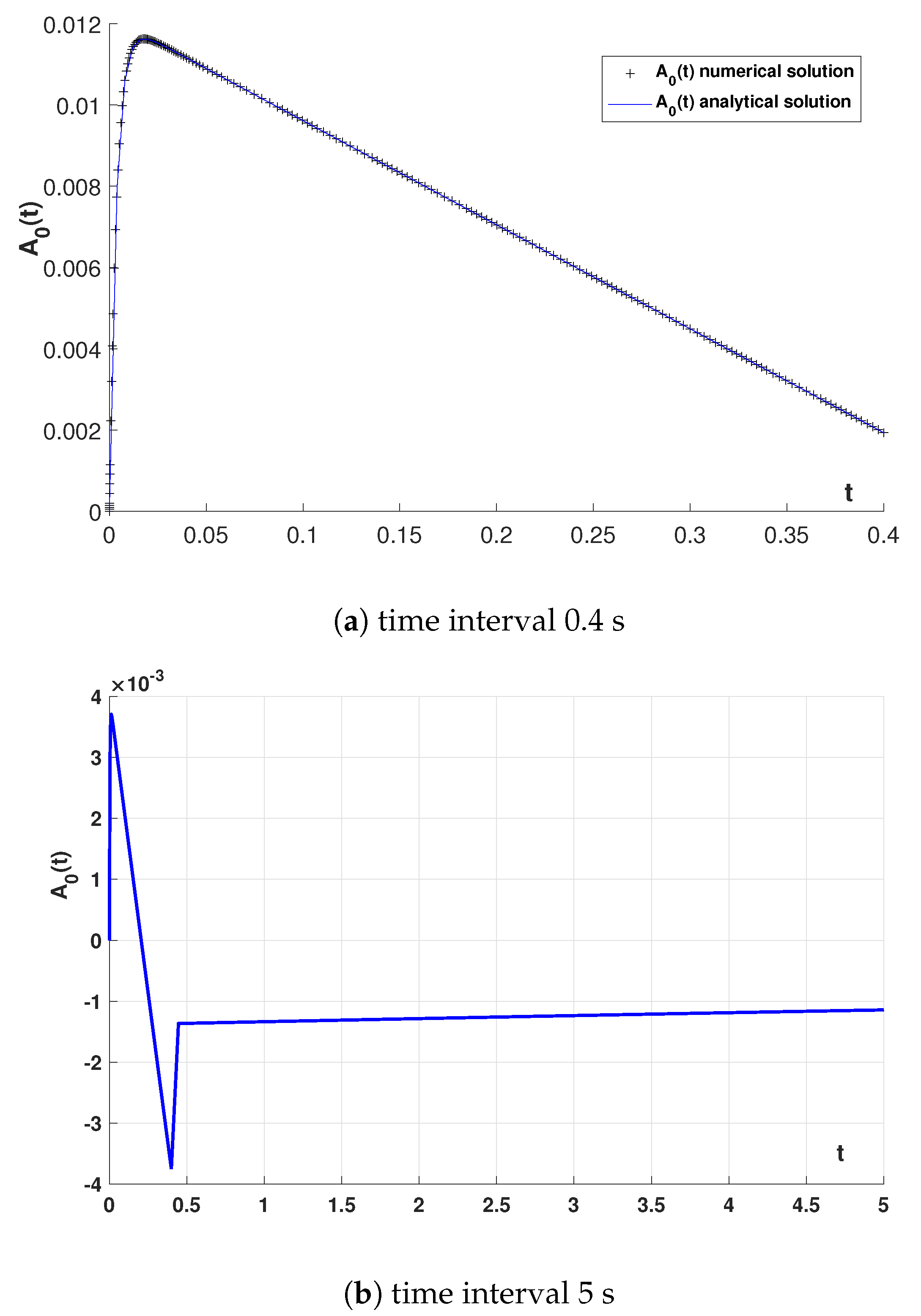
The amplitude $A_0\left(t\right)$ analytically obtained in (36) and numerically computed using a Runge–Kutta method in MatLab was plotted on the same graph in Figure 2a. Because of the accuracy of the calculus, only one method was used in Figure 2b.

The maximum amplitude is measured a short time after braking ([0, 0.4] to [0, 0.8] seconds). As seen in Figure 2a, for a time interval of [0, 0.4], the free surface follows a slight climb and stagnation. Additionally, as seen in Figure 2b, the “quietness” of the waves inside the tank is observed.

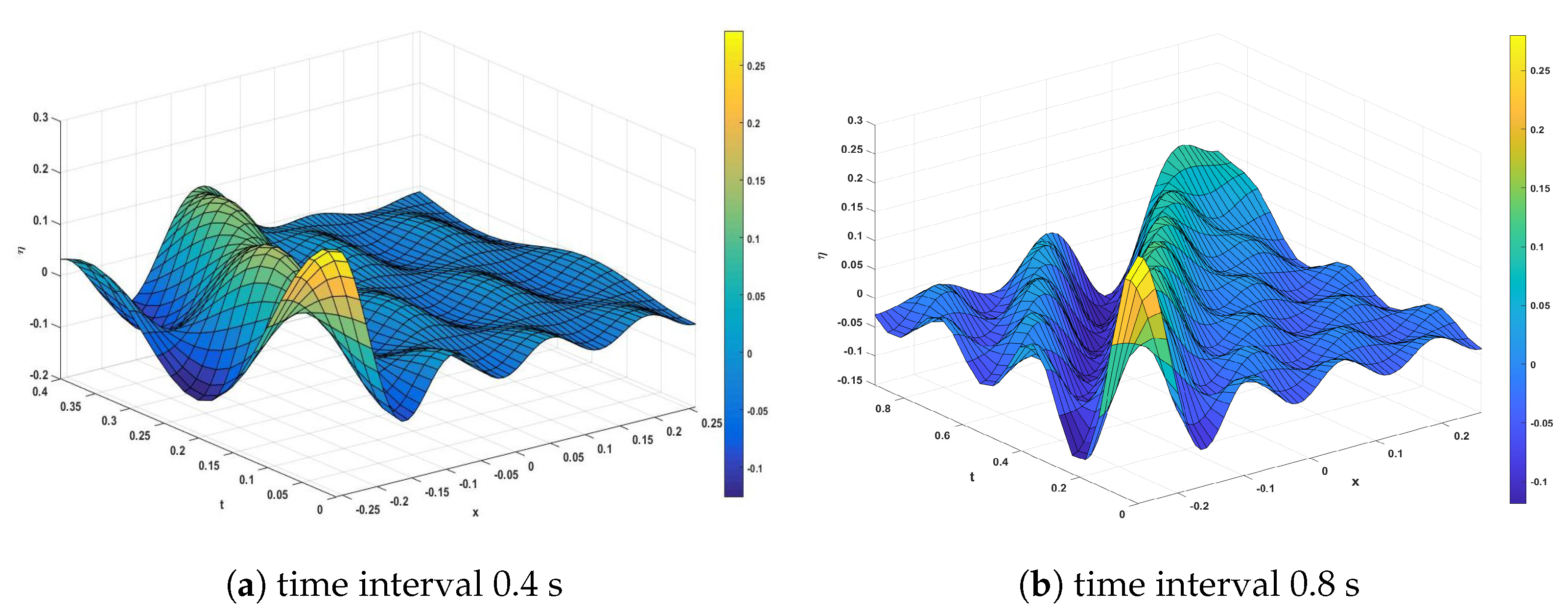
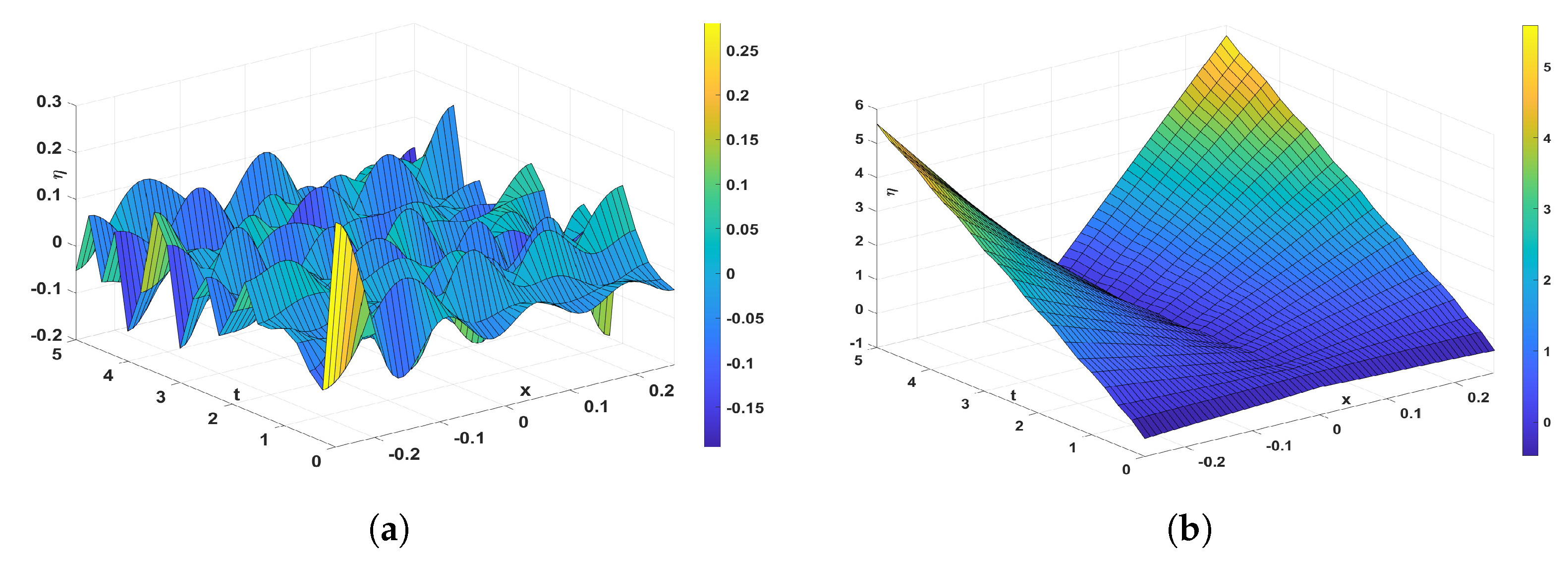
If a fuel tank does not contain wave breakers, a large wave is generated followed by successive smaller waves that will hit each other (Figure 3). The noise generated in this case represents the phenomenon of slosh noise, which is unpleasant for the user.

According to relation (36), when the time increases after $t_1$, the amplitude will be larger then the case $t<t_1$ if the term ${\displaystyle \frac{a}{{\omega }_1^2}}$ is bigger then the sum of the first two terms. That fact leads to the change of wave shape expressed in Figure 3.

As a remark, for Boussinesq’s non-linear model with a slight disturbance of amplitude, the linear conditions on the free surface will change [23]. Using cinematic condition (25) for any $\eta$, ${\displaystyle \frac{\partial \psi }{\partial t}+g\eta +ϵ\psi =0}$ and the dynamic condition for the free surface ${\displaystyle \frac{\partial \eta }{\partial t}-\frac{\partial \psi }{\partial y}=0}$, one finds the governing equation for the potential: ${\displaystyle \frac{{\partial }^2\psi }{\partial t^2}+ϵ\frac{\partial \psi }{\partial t}+g\frac{\partial \psi }{\partial y}=0.}$

In [12], the free surface elevation is made precise, the expression of the velocity potential of the first sloshing mode is given and the coefficient $ϵ$ was described by an approximation. The relative free surface elevations at the left wall with different excitation frequencies were numerically computed. We have analytically defined the time variation of the amplitude and the free surface inside the tank. Additionally, in [16], only numerical results were obtained.

4. Mathematical Model of the Fluid Flow in the Tank with a Slosh Noise Reduction Baffle

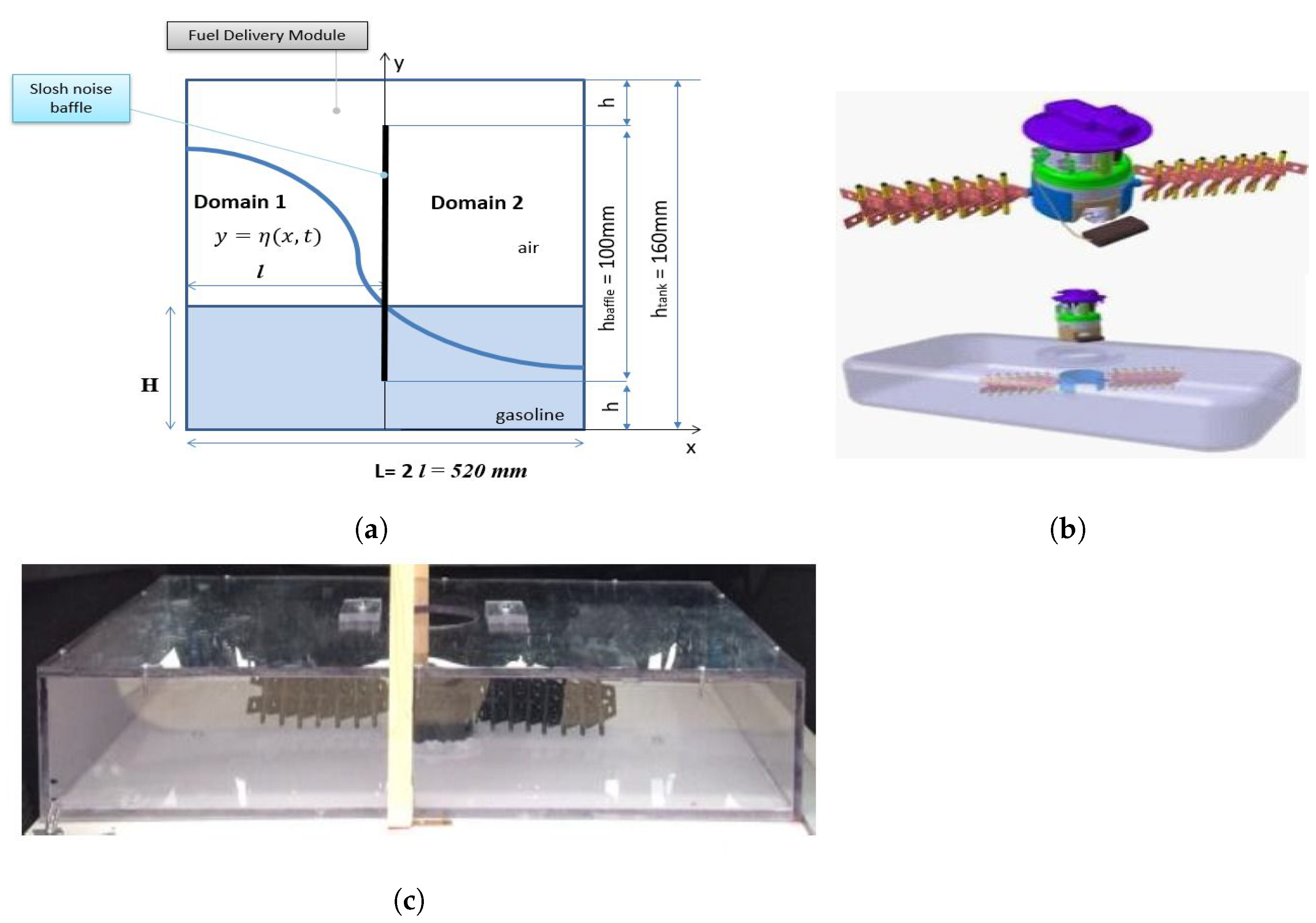
The initial status of a tank that includes a wave breaker is outlined in the Figure 4, where: h = 30 mm, tank length = 1000 mm, tank width (L) = 520 mm, and tank height = 160 mm.

We consider the movement of the free surface on the width of the tank as flat movement in the $xOy$ plane (in the transverse plane) and with the same values of the amplitude at any section along the length of the tank. According to the geometry shown in Figure 4a, with $sp$ = notation for the presence of a slosh noise baffle inside the tank and $fsp$ = notation for the case without the presence of a slosh noise baffle inside the tank, the movement in the tank is broken down into two areas: $\mathcal{D}=D_1\cup D_2$ with $D_1=[h,h+h_{sp}]\times [-l,0]$, $D_2=[h,h+h_{sp}]\times [0,l]$. The description of the geometry of the baffle for the experimental study (Figure 4b,c) is found in the patent, which is referenced within the paper at the beginning of Section 2.

The potential $\varphi =\phi +\psi$ check the Laplace equation with the shape (16) for $\phi$ and (20) for $\psi$ in both areas.

Taking into account the initial speed $U_0$ and the volume of liquid in the tank, one obtains an average value for the mass forces $f\left(t\right)=\int \frac{F}{m}dt=f_0\left(t\right)$, which will be used in the boundary conditions. According to the experimental approach and data, see [20], below are presented the values for the forces associated to the initial speed $U_0$.

The data from

Table 1. Parameter values of $f_0$ [N/kg] relative to the initial speed $U_0$.

Volume Liquid [L]	Mass [kg]	${\mathit{f}}_0$ [N/kg] at ${\mathit{U}}_0=10$ km/h	${\mathit{f}}_0$ [N/kg] at ${\mathit{U}}_0=30$ km/h	${\mathit{f}}_0$ [N/kg] at ${\mathit{U}}_0=50$ km/h
15	12.5	2.00800	2.28800	2.57600
25	20.9	2.00800	2.00000	2.27751
35	29.2	2.00342	2.28082	2.57192
45	37.6	2.0000	2.27926	2.56915

show the values for the forces, $f_0$, associated with different initial speeds, $U_0$ (10 km/h, 30 km/h, and 50 km/h) for three different volumes (15 L, 25 L, and 35 L) and corresponding masses (12.5 kg, 20.9 kg, and 29.2 kg) of a liquid. The forces are consistent across different speeds for the same volume and mass. The data show that the force decreases with increasing volume and mass of the liquid and that the force increases with increasing initial speed.

The boundary conditions on the $D_1$ side walls are:

$${\displaystyle \frac{\partial \psi }{\partial x}(-\frac{L}{2},y,t)=\dot{X}\left(t\right),\frac{\partial \psi }{\partial x}(0_{-},y,t)=f\left(t\right),y\in [h,h+h_{sp}],}$$

(39)

and on the $D_2$ side walls are

$${\displaystyle \frac{\partial \psi }{\partial x}(0_{+},y,t)=0,\frac{\partial \psi }{\partial x}(\frac{L}{2},y,t)=\dot{X}\left(t\right),y\in [h,h+h_{sp}],}$$

(40)

also, on the floor of the tank, the condition imposed is:

$${\left.{\displaystyle \frac{\partial \psi }{\partial y}}\right|}_{y=0}=0.$$

(41)

The first condition in (39) and the last condition in (40) expressed for ${\displaystyle \frac{\partial \psi }{\partial x}}$ express the condition on the wall of the tank, in which case the fluid will have the velocity of the tank described by $\dot{X}\left(t\right)$. On the left side of the baffle, the mass forces are considered identically distributed on the baffle using $f_0\left(t\right)$.

Using the inertia coefficient C and the drag coefficient $\alpha ={\left({\displaystyle \frac{1}{P{C}_c}-1}\right)}^2$ described through the porosity of the breaker (see [5]) and the discharge coefficient $C_c$, the jump condition on the sides of the breaker is:

$${\displaystyle {\left[{\displaystyle \frac{\partial \psi }{\partial t}(x,y,t)}\right]}_{-}^{+}=\frac{\alpha }{2}\frac{\partial \psi }{\partial x}\left|{\displaystyle \frac{\partial \psi }{\partial x}}\right|+2C\frac{{\partial }^2\psi }{\partial x\partial t}.}$$

(42)

and C is negligible if the thickness of the wave breaker is neglected.

On the other hand, the condition of the speed continuity at the level of $y=h$ expressing that the speed is continuous when passing from the level $y<h$ to $y=h$. For $y<h$, the liquid is without a wave breaker and the speed solution is known at the free surface $y=h$, in each domain ($D_1$ and $D_2$) determined by the separation of the baffle:

$${\displaystyle \frac{\partial \psi }{\partial x}={\left.u_{fsp}(x,y,t)\right|}_{y=h},x\in [-l,0],\mathrm{for\; determining\; the\; solution\; in} D_1,}$$

(43)

$${\displaystyle \frac{\partial \psi }{\partial x}={\left.u_{fsp}(x,y,t)\right|}_{y=h},x\in [0,l],\mathrm{for\; determining\; the\; solution\; in} D_2,}$$

(44)

where ${\displaystyle u^{fsp}(x,t)=\frac{\partial {\psi }^{fsp}}{\partial x}(x,h,t)}$, ${\psi }^{fsp}$ being the potential solution of the form (20) for the problem of the motion without a breaker.

According to the previously determined solution, we find that:

$${\displaystyle \begin{array}{c}{\displaystyle u^{fsp}(x,t)=-at+\sum _n{u}_n^{fsp}(x,t),t\in [0,t_1],}\hfill \\ u^{fsp}(x,t)=-a{t}_1+\sum _n{u}_n^{fsp}(x,t),t\in [t_1,t_s],\end{array}}$$

(45)

where

$${\displaystyle u_{nfsp}(x,y,t)=\frac{\partial {\psi }_n^{fsp}}{\partial x}(x,y,t)=\frac{\partial f_n^{fsp}}{\partial x}(x,y)sin\left({\omega }_n^{fsp}t\right),t\in [0,t_s].}$$

(46)

and for any $t\in [0,t_s]$, we have

$$u_n^{fsp}(x,t)={\left.u_{nfsp}(x,y,t)\right|}_{y=h}=K_n{\lambda }_{n}cosh\left({\lambda }_{n}H\right)sin\left({\lambda }_n(x+l)\right)sin\left({\omega }_n^{fsp}t\right).$$

(47)

(see [4]).

Additionally, the hydrostatic pressure and free surface can be described by:

$${\displaystyle p=-g\frac{\partial \psi }{\partial t},\eta =\frac{p}{\rho g}.}$$

(48)

The solutions of the potential function in the two areas are:

$${\psi }^1={\psi }_0^1+{\psi }_f,x\in [-l,0],\mathrm{respectively},{\psi }^2={\psi }_0^2+{\psi }_f,x\in [0,l],$$

(49)

with ${\psi }_f={\sum }_{n-1}^{\infty }{\psi }_n$, where ${\psi }_n=f_n^1(x,y)sin\left({\omega }_n^{sp}t\right)$ has solution type (21), $n\ge 1$,

$$f_n^1(x,y)=-C_{n}cos\left({\lambda }_n^{sp}(x+l)\right)cosh\left({\lambda }_n^{sp}H\right),$$

(50)

$f_n^1$ is a fundamental solution that verifies:

$${\displaystyle \Delta f_n^1=0,\frac{\partial f_n^1}{\partial x}\left(-l,y\right)=0=\frac{\partial f_n^1}{\partial x}(0,y),\frac{\partial f_n^1}{\partial y}{|}_{y=0}=0}$$

(51)

For the functions ${\psi }_0^1$ in the $D_1$ domain and ${\psi }_0^2$ in the $D_2$ domain, we have obtained for $\forall y\in [h,h+h_{sp}]$, $t\in [0,t_1]$ the solutions

$${\displaystyle {\psi }_0^1=A_{01}^1\left(t\right)+{\int }_0^1\frac{1}{{\omega }_1^{sp}}\left[-a(1-\theta )+f_0\theta \right]d\theta +x\left((U_0-at)(1-\theta )+f_{0}t\theta \right),}$$

(52)

when $x\in [-l,0]$ and

$${\displaystyle {\psi }_0^2=A_{01}^2\left(t\right)+{\int }_0^1\frac{1}{{\omega }_1^{sp}}\left[f_0(1-\theta )-a\theta \right]d\theta +x\left(f_{0}t(1-\theta )+(U_0-at)\theta \right)}$$

(53)

when $x\in [0,l]$, for ${\displaystyle \theta =\frac{t}{t_1}}$.

For $t\in [t_1,t_s]$ and denoting ${\displaystyle \theta =\frac{t-t_1}{t_s-t_1}}$, the functions ${\psi }_0^1$ and ${\psi }_0^2$ have the shape

$$\begin{array}{c}{\psi }_0^1=A_{02}^1\left(t\right)+x\left((U_0-at)(1-\theta )+f_{0}t\theta \right),\forall x\in [-l,0],\hfill \\ {\psi }_0^2=A_{02}^2\left(t\right)+x\left(f_{0}t(1-\theta )+(U_0-at)\theta \right),\forall x\in [0,l],\hfill \end{array}$$

(54)

where $A_{01}^2\left(t\right)=A_{01}^1\left(t\right)=c_{11}{e}^{r_{1}t}+c_{12}{e}^{r_{2}t};A_{02}^2\left(t\right)=A_{02}^1\left(t\right)=c_{21}{e}^{r_{1}t}+c_{22}{e}^{r_{2}t}$.

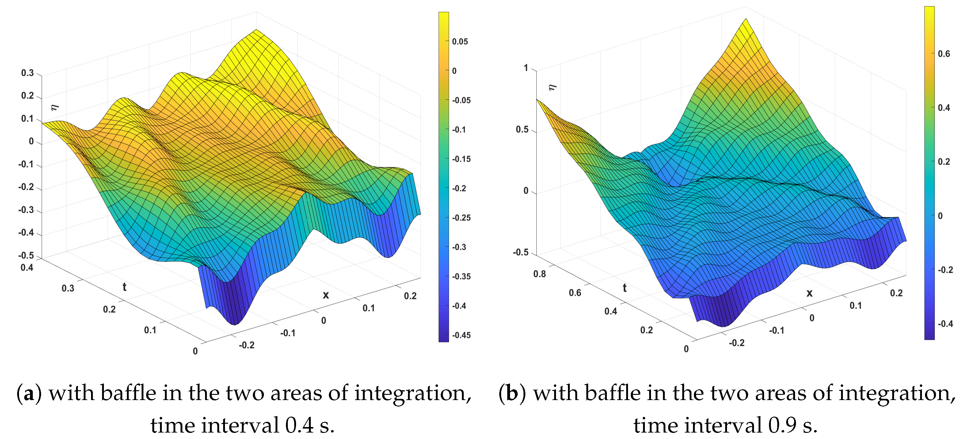
The free surface, depicted in Figure 5 for $t\in [0,0.4]$ s and $t\in [0,0.9]$ s, is determined by the relationship ${\displaystyle \frac{\partial \eta }{\partial t}+g\eta =0}$ for $y=\eta (x,t)$, with ${\eta }^i={\eta }_0^i+{\sum }_n{\eta }_n^i(x,t)$ and $i=1,2$ the free surfaces in the two domains $D_1$ and $D_2$.

According with the method of fundamental solutions used in (20), we obtain:

$${\displaystyle {\eta }_0^i=-\frac{1}{g}\frac{\partial {\psi }_0^i}{\partial t}-\frac{1}{g}\frac{\partial {\psi }_f}{\partial t},i=1,2.}$$

(55)

where

$${\displaystyle -\frac{1}{g}\frac{\partial {\psi }_f}{\partial t}=\sum _{n=0}^{\infty }Hcos\left({\lambda }_n^{sp}(x+l)\right)cos\left({\omega }_n^{sp}t\right)}$$

(56)

Additionally, for $t\in [0,t_1]$, we have

$${\displaystyle \begin{array}{c}{\displaystyle -\frac{1}{g}\frac{\partial {\psi }_0^1}{\partial t}=-\frac{1}{g}\left[{\dot{A}}_{01}^1\left(t\right)+x\left({\displaystyle -a+2(f_0+a)\frac{t}{t_1}-\frac{U_0}{t_1}}\right)\right],\forall x\in [-l,0],}\hfill \\ {\displaystyle -\frac{1}{g}\frac{\partial {\psi }_0^2}{\partial t}=-\frac{1}{g}\left[{\dot{A}}_{01}^2\left(t\right)+x\left({\displaystyle f_0+\frac{U_0}{t_1}-2(f_0+a)\frac{t}{t_1}}\right)\right],\forall x\in [0,l],}\hfill \end{array}}$$

(57)

and for $t\in [t_1,t_s]$, one obtains

$$\begin{array}{c}{\displaystyle -\frac{1}{g}\frac{\partial {\psi }_0^1}{\partial t}=-\frac{1}{g}\left[{\dot{A}}_{02}^1\left(t\right)+x\left({\displaystyle -a+2(f_0+a)\frac{t}{t_s-t_1}-\frac{U_0}{t_1}}\right)\right],\forall x\in [-l,0],}\hfill \\ {\displaystyle -\frac{1}{g}\frac{\partial {\psi }_0^2}{\partial t}=-\frac{1}{g}\left[{\dot{A}}_{02}^2\left(t\right)+x\left({\displaystyle f_0+\frac{U_0}{t_1}-2(f_0+a)\frac{t}{t_s-t_1}}\right)\right],\forall x\in [0,l].}\hfill \end{array}$$

(58)

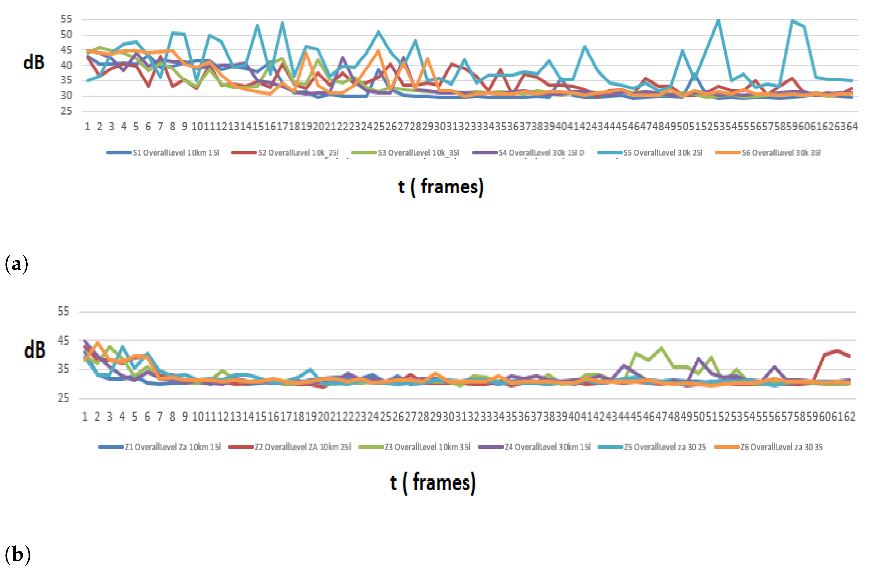
The relationships developed, (57) and (58), indicate a dependency of the height and number of waves created within a vehicle tank on the presence or absence of a wave breaker, its geometry also being important. The same dependency was also determined experimentally, following the measurement of the noise level recorded under different running conditions, according to the data in

Table 2. Initial conditions for the cases considered during acoustic measurements.

No.	Case	Presence of Baffle	Volum of Liquid [L]	Speed before Braking [km/h]
1	S1	no baffle	15	10
2	S2	no baffle	15	30
3	S3	no baffle	25	10
4	S4	no baffle	25	30
5	S5	no baffle	35	10
6	S6	no baffle	35	30
7	S7	no baffle	45	10
8	S8	no baffle	45	30
9	F1	Baffle included	15	10
10	F2	Baffle included	15	30
11	F3	Baffle included	25	10
12	F4	Baffle included	25	30
13	F5	Baffle included	35	10
14	F6	Baffle included	35	30
15	F7	Baffle included	45	10
16	F8	Baffle included	45	30

.

In [24,25], a correlation between the sound intensity due to sloshing and the pressure fluctuation dp/dt has been found, and connecting to (49), ${\displaystyle \frac{\partial \eta }{\partial t}=\frac{1}{\rho g}\frac{\partial p}{\partial t}}$, the variation in time and space was depicted in Figure 5.

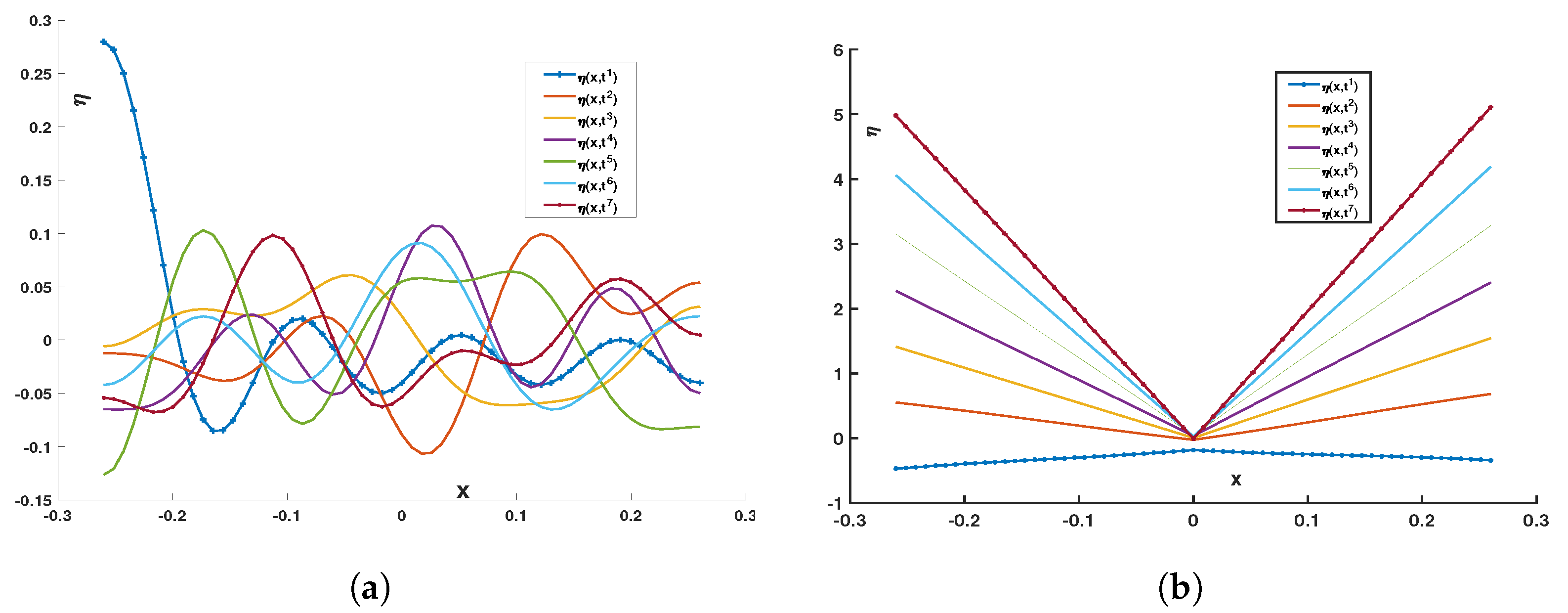
According to Figure 5, when a tank has a wave breaker, a single large wave is observed and the liquid tends to move towards the sides. Theoretically, by incorporating a wave breaker into a tank, the noise caused by the sloshing phenomenon is reduced due to the lack of waves. By analysing Figure 6 and Figure 7, it can be seen that the free surface behaves differently, with a significant reduction in the number of waves in the case of a wave breaker being integrated. This results in a reduction in the discomfort caused by the sloshing phenomenon. Negative values on the X-axis are a result of the chosen axis system, where −0.25 m and +0.25 m represent the tank walls.

The reference level is set to the level of the liquid at rest (H level, as seen in Figure 1b and Figure 4b) and positive and negative variations from this level are observed after braking.

As can be seen in Figure 7a, there are ripples on the free surface, these being unfractionated surfaces (the gradient on the curves does not change its convexity), which are smoother, and thus no noise is generated by the collision of small waves. The greater the distance between two peaks of the amplitude, the flatter the free surface is, and thus non-noisy.

In the considered model, the study is carried out in the centre of the tank, not taking into account that the vehicle tanks have an upper limit, given by the tank ceiling. For future research, it is an advanced study taking into account the model’s upper limitation, considering that when the wave returns, the potential movement becomes turbulent.

All the graphics in the paper were created by the authors, and the computations were made using MatlabR2022b codes.

5. Conclusions and Future Researches

For people travelling in a car with a stop-start system, the slosh noise caused by the movement of fuel in the tank is considered to be an annoyance. The intensity of this phenomenon increases during braking and accelerating.

The paper studies the movement of fuel in the tank, analysing both the waves and the sound generated during the accelerating and braking of the car. The associated phenomenon, called the slosh noise effect, is studied through analytical and approximate models. The analytical mathematical model of the free surface of the fluid during movement includes the determination of the potential function and the velocity components, in two different variants, with and without wave breakers. The model of the fuel movement in a tank containing wave breakers (baffles) was developed by dividing the fuel volume into two regions, separated by the baffle surfaces and defining both boundary and jump conditions on the baffle surfaces.

Based on the analytical models (for tanks with and without baffles), graphical representations of the free surface movement were made in both variants, with and without baffles. Comparing the graphs of the waves in each case, it is observed that the introduction of the baffles reduces the phenomenon by half (see Section 4). Thus, it is found that the amplitude of the movement of the free surface of the fluid in the case of the implementation of a wave breaker solution of the type of baffle is reduced by half compared to the movement of the free surface of the fluid contained in a fuel tank that does not present anti-blinking technical solutions.

The theme represents the creation of a new baffle design for fuel tanks in the automotive industry that can be adapted to already existing fuel tanks without modifying the original design. The baffle is needed to decrease noise generated by the fuel waves inside the fuel tank. Its effect is shown in Figure 8, confirmed by physical experimental tests [20].

The comparative analysis by the amplitude and free surface leads to new future research directions on the correspondence between free surface movement and the noise level generated through the module of the velocity, and the nondimensional simplified form of the Bernoulli integral for incompressible flows:

$${\displaystyle \frac{1}{2}{\left({\mathbf{v}}^{fsp}\right)}^2+\frac{{\left(c^{fsp}\right)}^2}{\gamma -1}=\frac{1}{2}{\left({\mathbf{v}}^{sp}\right)}^2+\frac{{\left(c^{sp}\right)}^2}{\gamma -1},}$$

with $\gamma$ being the ratio between specific heat at constant pressure and specific heat at constant volume [1,26]. The Bernoulli integral allows us to make the connection between the velocity of the fuel and the level of the sound due to the waves in the tank. As one observes from the previous formula, for a smaller module of the velocity ${\mathbf{v}}^{fsp}=\sqrt{u_{fsp}^2+v_{fsp}^2}$ results in a larger value for the sound speed and also in a larger value of the velocity module when the wave breaker is introduced, meaning ${\mathbf{v}}^{sp}=\sqrt{u_{sp}^2+v_{sp}^2}$, then the speed sound becomes smaller.

According with our notations, $\mathbf{v}{}^{sp}=(u_{sp},v_{sp})$ and $\mathbf{v}{}^{isp}=(u_{sp}^i,v_{sp}^i)$ with $i=1,2$, is the velocity corresponding to the two domains $D_1$ and $D_2$ (see Section 4). For $t\in [0,t_1]$ and any $y\in [h,h+h_{sp}]$, we have

$$\begin{array}{c}{\displaystyle u_{sp}^1=\frac{\partial {\psi }_0^1}{\partial x}=(U_0-at)(1-\theta )+f_{0}t\theta }\hfill \\ {\displaystyle +\sum _{n=1}^{\infty }\frac{C_n}{{\lambda }_n^{sp}}sin\left({\lambda }_n^{sp}(x+l)\right)cosh\left({\lambda }_n^{sp}y\right)sin\left({\omega }_n^{sp}t\right),\theta =\frac{t}{t_1}}\hfill \\ {\displaystyle v_{sp}^1=\frac{\partial {\psi }_0^1}{\partial y}=-\sum _{n=1}^{\infty }\frac{C_n}{{\lambda }_n^{sp}}cos\left({\lambda }_n^{sp}(x+l)\right)sinh\left({\lambda }_n^{sp}y\right)sin\left({\omega }_n^{sp}t\right),}\end{array}$$

(59)

and also for $t\in [t_1,t_s]$ and any $y\in [h,h+h_{sp}]$, the velocity components are

$$\begin{array}{c}{\displaystyle u_{sp}^2=\frac{\partial {\psi }_0^2}{\partial x}=(U_0-at)\theta +f_{0}t(1-\theta )}\hfill \\ {\displaystyle +\sum _{n=1}^{\infty }\frac{C_n}{{\lambda }_n^{sp}}sin\left({\lambda }_n^{sp}(x+l)\right)cosh\left({\lambda }_n^{sp}y\right)sin\left({\omega }_n^{sp}t\right),\theta =\frac{t-t_1}{t_s-t_1}}\hfill \\ {\displaystyle v_{sp}^2=\frac{\partial {\psi }_0^2}{\partial y}=-\sum _{n=1}^{\infty }\frac{C_n}{{\lambda }_n^{sp}}cos\left({\lambda }_n^{sp}(x+l)\right)sinh\left({\lambda }_n^{sp}y\right)sin\left({\omega }_n^{sp}t\right).}\hfill \end{array}$$

(60)

Figure 8, expressing the result of the experimental study, and Figure 3, Figure 5, Figure 6 and Figure 7, describing the results of the analytical study, lead to the conclusion that the use of the baffle reduces the slosh noise, improving the efficiency of the tank usage. Figure 3a is compared with Figure 5a, and Figure 3b is compared with Figure 5b.

For future studies, we aim to analyse the energy behaviour of the system through potential energy defined in (12) and kinetic energy defined in (13) that, for the case with the breaker solution implemented, becomes

$$\begin{array}{c}{\displaystyle U_{sp}^e=\frac{1}{2}\rho gb\left({\int }_{-l}^0{\left({\eta }_0^1\right)}^2(x,t)+{\int }_0^l{\left({\eta }_0^1\right)}^2(x,t)\right)\mathrm{d}x,}\hfill \\ {\displaystyle T_{sp}^e=\frac{1}{2}\rho g{\int }_V{(\nabla {\psi }_{sp})}^2\mathrm{d}V.}\hfill \end{array}$$

(61)

and compare the two solutions from this point of view.

References

1. Dragos, L. Introducere Matemation in Mecanica Fluidelor/Mathematical Introduction in Fluid Mechanics; Romanian Academy Press: Bucharest, Romania, 2000. [Google Scholar]
2. Fox, R.W.; McDonald, A.T.; Pritchard, P.J. Introduction in Fluid Mechanics, 6th ed.; John Wiley Sons: New York, NY, USA, 2004; ISBN 0-471-37653-1. [Google Scholar]
3. Chu, C.R.; Wu, Y.R.; Wu, T.R.; Wang, C.Y. Slosh -induced hydrodynamic force in a water tank with multiple baffles. Ocean Eng. 2018, 167, 282–292. [Google Scholar] [CrossRef]
4. Cho, I.H.; Kim, M.H. Effect of dual porous baffles on sloshing reduction in a swaying rectangular tank. Ocean Eng. 2016, 126, 364–373. [Google Scholar] [CrossRef]
5. Poguluri, S.K.; Cho, I.H. Liquid sloshing in a rectangular tank with vertical slotted porous screen: Bassed on analytical, numerical and experimental approach. Ocean Eng. 2019, 189, 106–373. [Google Scholar] [CrossRef]
6. Lu, L.; Jiang, S.C.; Zhao, M.; Tang, G.Q. Two-dimensional viscous numerical simulation of liquid sloshing in rectangular tank with/ without baffles and comparison with potential flow solutions. Ocean Eng. 2015, 108, 662–667. [Google Scholar] [CrossRef]
7. Shao, J.R.; Li, H.Q.; Liu, G.R.; Liu, M.B. An improved sph method for modeling liquid sloshing dynamics. Comput. Struct. 2012, 100–101, 18–26. [Google Scholar] [CrossRef]
8. Hassan, H.A.S. Muti dimensional nurbs model for predicting maximum free surface oscilation in swaying rectangular storage tanks. Comput. Math. Appl. 2018, 76, 2496–2513. [Google Scholar] [CrossRef]
9. Wang, L.; Xu, M.; Zhang, Q. Numerical Investigation of Shallow Liquid Sloshing in a Baffled Tank and the Associated Damping Effect by BM-MPS Method. J. Mar. Sci. Eng. 2021, 9, 1110. [Google Scholar] [CrossRef]
10. Koli, G.C.; Kulkarni, V.V. Simulation of Fluid Sloshing in a Tank, World Congress on Engineering (WCE 2010); Imperial Coll London: London, UK, 2010; Volume II, pp. 1028–1033, LECT NOTES ENG COMP, INT ASSOC ENGINEERS-IAENG; ISBN 978-988-18210-7-2. ISSN 2078-0958. [Google Scholar]
11. Frosina, E.; Senatore, A.; Andreozzi, A.; Marinaro, G.; Buono, D.; Bianco, G.; Auriemma, D.; Fortunato, F.; Damiano, F.; Giliberti, P. Study of the sloshing in a fuel tank using CFD and EFD approaches. In Proceedings of the ASME/BATH 2017 Symposium on Fluid Power and Motion Control (FPMC2017), Sarasota, FL, USA, 16–19 October 2017; ISBN 978-0-7918-5833-2. [Google Scholar]
12. Yan, S.; Liu, Z.Y. Numerical model of sloshing in rectangular tank based on boussinesq type equations. Ocesn Eng. 2016, 121, 166–173. [Google Scholar] [CrossRef]
13. Lin, B.H.; Chen, B.F.; Tsai, C.C. Method of fundamental solutions on simulating sloshing liquids in a 2d tank. Comput. Math. Appl. 2019, 88, 52–69. [Google Scholar] [CrossRef]
14. Matsson, J. Ansys 19.1 Relesse Notes, SAS IP; Version 19.1; SDC Publications: Mission, KS, USA, 2018. [Google Scholar]
15. Arafa, M. Finite element snalysis of sloshing in rectangular liquid-filled tanks. J. Vib. Control 2007, 13, 883–903. [Google Scholar] [CrossRef]
16. Demirel, E.; Aral, M.M. Liquid sloshing damping in an accelerated tank using a novel slot baffle design. Water 2018, 10, 1565. [Google Scholar] [CrossRef]
17. Hallez, R.l.; McGann, I.F.; Sibal, S.D.; Li, F. Radiated Fuel Tank Slosh Noise Simulation; SAE Internationa: Warrendale, PA, USA, 2011. [Google Scholar] [CrossRef]
18. Charpentier, A.; Kim, H.; Hwang, Y.; Noh, J.; Caro, S. Validation of Fuel Tank Slosh Noise and Vibration Predictions. In Proceedings of the INTER-NOISE and NOISE-CON Congress and Conference Proceedings, Hamburg, Germany, 21–24 August 2016. [Google Scholar]
19. Frosina, E.; Senatore, A.; Andreozzi, A.; Fortunato, F.; Giliberti, P. Experimental and Numerical Analyses of the Sloshing in a Fuel Tank. Energies 2018, 11, 682. [Google Scholar] [CrossRef]
20. Manta, O.M.; Balas, R.; Ulmeanu, M.E.; Murzac, R.; Doicin, C.V. Construction and testing of the wave breaking prototype—Slosh noise baffle. UPB Sci. Bull. 2022, 84, 103–116. [Google Scholar]
21. Manta, O.M.; Balas, R.; Murzac, R.; Ulmeanu, M.; Doicin, C.V. Statical Analysis of Slosh Noise Baffle, Macromolecular Symposia. In Proceedings of the International Conference on Design and Technologies for Polymeric and Composite Products (POLCOM), Bucharest, Romania, 10–11 October 2019; WILEY-V C H VERLAG GMBH: Weinheim, Germany, 2020. [Google Scholar] [CrossRef]
22. Manta, M.; Balas, R.; Doicin, C.V. Research and constructive solutions on the reduction of slosh noise, 20th Innovative Manufacturing Engineering and Energy Conference (IMANEE 2016). In Proceedings of the IOP Conference Series-Materials Science and Engineering, Kallithea, Greece, 23–25 September 2016; IOP Publishing Ltd.: Bristol, UK, 2016. [Google Scholar]
23. Matsson, J. ANSYS Software User’s Guide 15.0, SAS IP; Version 15.0; SDC Publications: Mission, KS, USA, 2013. [Google Scholar]
24. Wiesche, S.A.D. Noise due to sloshing within automotive fuel tanks. Forsch. Ing. 2006, 70, 13–24. [Google Scholar] [CrossRef]
25. Agawane, G.; Jadon, V.; Balide, V.; Banerjee, R. An Experimental Study of Sloshing Noise in a Partially Filled Rectangular Tank. SAE Int. J. Passeng. Cars-Mech. Syst. 2017, 10, 391–400. [Google Scholar] [CrossRef]
26. Milne-Thomson, L.M. Theoretical Hydrodynamics, 4th ed.; MacMillan Co., Ltd.: London, UK, 1962. [Google Scholar]
Figure 1. Tank geometry. (a) Geometry of a non-stop tank used for the analytical model. (b) Geometry of a non-stop tank for the experimental study.
Mathematics 11 00949 g001
Figure 2. Evolution of amplitude (A0 [m]) (a) time t [ 0 , 0.4 ]   s , (b) time t [ 0 , 5 ]   s .
Mathematics 11 00949 g002
Figure 3. Evolution of the free surface (a) t [ 0 , 0.4 ]   s , (b) time t [ 0 , 0.8 ]   s .
Mathematics 11 00949 g003
Figure 4. Geometry of a slosh noise baffle integrated in the tank. (a) The geometry of the baffle tank used for (MA). (b) Assembly of the baffle in the tank. (c) The geometry of the baffle tank used for experimental study.
Mathematics 11 00949 g004
Figure 5. Evolution of the free surface (a) t [ 0 , 0.4 ]   s , (b) time t [ 0 , 0.9 ]   s .
Mathematics 11 00949 g005
Figure 6. Evolution of wave amplitude (free surface section in direction X). (a) Evolution of wave amplitude for a tank without a baffle. (b) Evolution of wave amplitude for a tank with a breaker included.
Mathematics 11 00949 g006
Figure 7. Evolution of wave amplitude. (a) Behaviour of the free surface for a slosh noise baffle-free tank. (b) Behaviour of the free surface for a slosh noise baffle in the tank.
Mathematics 11 00949 g007
Figure 8. Noise variation based on a technical solution implemented inside the tank. (a) Fuel tank without any slosh noise solution. (b) Patented slosh noise baffle integrated in the tank.
Mathematics 11 00949 g008