On-Orbit Verification of RL-Based APC Calibrations for Micrometre Level Microwave Ranging System

Abstract

Micrometre level ranging accuracy between satellites on-orbit relies on the high-precision calibration of the antenna phase center (APC), which is accomplished through properly designed calibration maneuvers batch estimation algorithms currently. However, the unmodeled perturbations of the space dynamic and sensor-induced uncertainty complicated the situation in reality; ranging accuracy especially deteriorated outside the antenna main-lobe when maneuvers performed. This paper proposes an on-orbit APC calibration method that uses a reinforcement learning (RL) process, aiming to provide the high accuracy ranging datum for onboard instruments with micrometre level. The RL process used here is an improved Temporal Difference advantage actor critic algorithm (TDAAC), which mainly focuses on two neural networks (NN) for critic and actor function. The output of the TDAAC algorithm will autonomously balance the APC calibration maneuvers amplitude and APC-observed sensitivity with an object of maximal APC estimation accuracy. The RL-based APC calibration method proposed here is fully tested in software and on-ground experiments, with an APC calibration accuracy of less than 2 mrad, and the on-orbit maneuver data from 11–12 April 2022, which achieved 1–1.5 mrad calibration accuracy after RL training. The proposed RL-based APC algorithm may extend to prove mass calibration scenes with actions feedback to attitude determination and control system (ADCS), showing flexibility of spacecraft payload applications in the future.

1. Introduction

Micrometre level, or even nanometre, picometre level high-precision on-orbit inter-satellite ranging (ISR) technology constituted the foundation stone for modern space science exploration missions. Application of precise ISR technology, including gravitational wave detection that extended Einstein’s theory of relativity in a more general form [1,2,3], and the Earth gravity field measurement that learned the spatial and temporal distribution of Earth’s internal mass [4,5].

Realization of high accuracy ISR can be achieved through an optical phase measurement-based laser interferometric technique, as in LISA Pathfinder and GRACE follow-on missions [6,7,8,9]. At the same time, the dual one-way ranging (DOWR)-based K/Ka band dual frequency microwave phase differential measurement technique is also used, and even functioned as the primary ISR payload in current on-orbit missions [10,11].

The high-accuracy ISR measurement from laser, or microwave payload suffered from noises and perturbations, which should be precisely modeled and calibrated, both before and after launch. The calibrating process, referred to as line-of-sight (LOS) calibration for laser ranging interferometer (LRI) [12], or APC calibration for microwave ranging payloads [13], is one crucial initial ranging acquisition procedure that includes well-designed spacecraft maneuvers and algorithms. The purpose of APC calibration is for the optimal estimation of the microwave antenna phase center on board the formation spacecrafts. The whole calibration procedure entails the intended attitude orientation through ADCS functioning, optimal design of maneuver parameters, proper choice of APC estimation algorithms, and finally, obtaining the alignment corrections of precise ranging information between the inertial proof mass of formation spacecrafts.

The traditional way of conducting APC calibration is by the command sending and receiving through ground telemetry, the track and command (TT&C) system, with predetermined maneuver parameters. However, one problem arises during real APC calibration on-orbit. The K/Ka band dual frequency antennae on board are sophisticatedly designed horns with a sharp pattern in the main lobe, aiming to obtain high gain values in the LOS direction. However, the APC is only sensitive to the sweep plan of the maneuver spacecraft with large rotating angles; on the one hand, too-large maneuver angles cause microwave ranging performance to deteriorate. However, angles that are too small would fail to obtain precise APC information. A similar situation also exists in the center of mass (CoM) calibration process on-orbit, which causes a dilemma. With the rapid development of artificial intelligence (AI), machine learning (ML) and reinforcement learning (RL) technology in recent years, it is interesting to explore the possible applications of those methods to the APC calibration on-orbit.

Reinforcement learning, a major branch of machine learning, has attracted scholars’ attention over the last decade. RL functioned adaptively to formulate a ’policy update’ through interactions with an environment [14]. Of the copious literature related to RL studies, policy gradient methods are a group of practical algorithms that are commonly used and well established [15,16]. The core idea of the RL process is to seek to maximize the performance index with respect to the parameters from the policy function by using gradient descent. Readers can refer to the aforementioned policy gradient method [16], off-policy actor-critic method and trust region optimization [17,18]. Application of RL to an aerospace system is rarely found in recent years, and some newly relevant literature may be found in [19,20,21].

Despite the rare application of reinforcement learning in the Microwave ranging (MWR) systems, this paper provides an early attempt to conduct RL-based APC calibration for micrometre level precision MWR ranging on-orbit. The main contributions of this study are summarized as follows: Detailed analysis of the APC calibration model with noises and uncertainties that are experienced in real on-orbit flights; Formulating the APC calibration as an on-orbit RL problem with related algorithm derivation; Verification of proposed RL APC algorithms with software simulation and the hardware in loop (HIL) test, and finally, with real on-orbit MWR data. The proposed RL-based APC process method may extend to a general form that includes proof mass calibration simultaneously.

The remainder of this paper is organized as follows: The mathematical models for APC calibrations with antenna bias analysis are provided in Section 2. The RL-based algorithm for APC calibration can be found in Section 3. The RL-based algorithm test using software, HIL and on-orbit verification are described in Section 4, Section 5 and Section 6, with discussion in Section 7.

2. Mathematical Models for Antenna Phase Center Calibration

2.1. APC Calibration Procedure

2.1.1. Sub-Maneuvers Design

Precise measurement of MWR payload depends on the accuracy on-orbit estimation of APC for both satellites. Due to the reason that the APC component is only sensitive to the values along the sweep plan of the satellite attitude rotating, maneuvers of several kinds should be adopted to determine the correct APC positions.

Similar to ref [13], here we provide four separate on-orbit calibration sub-maneuvers. The periodic oscillation maneuver is used as follows:

$${\theta }_{<y,p>}^{<a,b>}={\theta }_0+Asin\left(\omega t\right)$$

(1)

where $\theta$ is the angle during each sub-maneuver, the subscript $<y,p>$ denotes the sub-maneuvers of yaw or pitch angles, and $<a,b>$ denotes the satellite A or B that perform the sub-maneuver. The four sub-maneuvers are defined as Sub-Maneuver A (MA) ${\theta }_{yaw}^a$, MB ${\theta }_{pitch}^a$, MC ${\theta }_{yaw}^b$, MD ${\theta }_{pitch}^b$. ${\theta }_0$ is the initial biased attitude angle before each sub-maneuver, the reason for this is that the MWR ranging measurement is highly correlated to the attitude rotation with biased angle. The schematic illustration of this sub-maneuver is shown in Figure 1, taking MA as an example.

   Clearly, in the case of MA, the phase observation is highly sensitive to the phase center of spacecraft A’s antenna along roll and pitch axes. Here we did not model the bias of the satellites’ center of mass (CoM), which is supposed to coincide with the on-board accelerometer’s proof mass [22].

2.1.2. APC Calibration Algorithm

The required observation set for MWR system APC calibration includes precise micrometre level MWR range data, star camera data for attitude orientations determination for satellites A and B, and relative position measurements from GPS observations.

Same as chapter 4 of ref. [13], the range fitting model is given as

$$R=\left|{\mathbf{r}}_{ab}^{*}+\Re {\left({\mathbf{q}}_a\right)}^T\mathrm{\Theta }\left({\mathbf{d}}_{pca}\right)-\Re {\left({\mathbf{q}}_b\right)}^T\mathrm{\Theta }\left({\mathbf{d}}_{pcb}\right)\right|+R_{br}+R_{nr}+Poly\left(n\right)$$

(2)

where ${\mathbf{r}}_{ab}$ is GPS the determined relative position in the inertial frame, $\Re \left(•\right)$ denotes the operation of attitude quaternion to the rotation matrix, $\mathrm{\Theta }\left(•\right)$ the operation of the vertical vector to the horizontal, ${\mathbf{q}}_a,{\mathbf{q}}_b\in {\mathbb{S}}^3$ are the attitude quaternion of satellite A and B from the inertial frame to body-frame, ${\mathbf{d}}_{pca},{\mathbf{d}}_{pcb}\in {\mathbb{R}}^3$ the APC coordinate (m) of satellite A and B in each body-frame, $R_{br}\in {\mathbb{R}}^1$ the MWR system measurement noises (m) that include oscillator noise and multipath noise [23], $R_{nr}\in {\mathbb{R}}^1$ the random ranging noise (m) with $\mathbb{E}\left(R_{nr}\right)=0$ and covariance $\mathbb{E}\left(R_{nr}{R}_{nr}^T\right)={\mathbf{R}}_r$, $Poly\left(n\right)$ is the n-th order polynomial function $a_n{t}^n+\dots +a_{1}t+a_0$, which is used to smooth the relative GPS measurement. Detail definition of coordinate frames may found in Appendix A.

The derivative of Equation (2) include

$$\frac{\partial R}{\partial {\mathbf{d}}_{pca}}=\frac{\partial }{\partial {\mathbf{d}}_{pca}}\left[\Re {\left({\mathbf{q}}_a\right)}^T\mathrm{\Theta }\left({\mathbf{d}}_{pca}\right)\right]={\mathbf{e}}^T\Re \left({\mathbf{q}}_a\right)\stackrel{\Delta }{=}{\mathbf{e}}^T{\mathbf{M}}_a,$$

$$\frac{\partial R}{\partial {\mathbf{d}}_{pcb}}=\frac{\partial }{\partial {\mathbf{d}}_{pcb}}\left[-\Re {\left({\mathbf{q}}_b\right)}^T\mathrm{\Theta }\left({\mathbf{d}}_{pcb}\right)\right]=-{\mathbf{e}}^T\Re \left({\mathbf{q}}_b\right)\stackrel{\Delta }{=}-{\mathbf{e}}^T{\mathbf{M}}_b,$$

(3)

$$\frac{\partial R}{\partial R_{br}}=1,\frac{\partial R}{\partial a_i}=\frac{\partial }{\partial a_i}\left[a_n{t}^n+\dots +a_{1}t+a_0\right]=t^i\left(i=0,1,2,\dots n\right)$$

where $\mathbf{e}$ is the unit vector of the satellite AB baseline in inertial frame, $\mathbf{M}$ is the transformation matrix from the inertial frame to the satellite body-frame.

Here we define the high-dimensional states as

$${\mathbf{x}}_{30\times 1}={\left[\underset{1\times 6}{\underbrace{{\mathbf{d}}_{pca}^T,{\mathbf{d}}_{pcb}^T}},\underset{1\times 4}{\underbrace{R_{br}^{MA},\dots R_{br}^{MD}}},\underset{1\times 20}{\underbrace{a_i^{MA},\dots a_i^{MD}}}\right]}^T.$$

Supposing we have the initial value ${\mathbf{x}}^{*}$ and measurement, then the residual of each sub-maneuver is the following:

$$y=R-\left|{\mathbf{r}}_{ab}^{*}+{\mathbf{M}}_a\mathrm{\Theta }\left({\mathbf{d}}_{pca}^{*}\right)-{\mathbf{M}}_b\mathrm{\Theta }\left({\mathbf{d}}_{pcb}^{*}\right)\right|-R_{br}^{*}-Poly{\left(n\right)}^{*},$$

(4)

with nominal values of marked *. The derivative matrix of the observed equation, for sub-maneuver A as an example is given as

$${\mathbf{H}}_{MA}=\left[\begin{array}{cccccccccc}\frac{\partial R_{MA}}{\partial {\mathbf{d}}_{pca}}& \frac{\partial R_{MA}}{\partial {\mathbf{d}}_{pcb}}& 1& 0& 0& 0& \frac{\partial R_{MA}}{\partial a_i^{MA}}& 0& 0& 0\end{array}\right].$$

(5)

A similar matrix can be obtained for other sub-maneuvers with the same method, and a fourth-order polynomial function is used here. By accumulating the measurements and derivative matrix for all sub-maneuvers, the following nominal matrix can be obtained:

$$\left({\mathbf{H}}^T{\mathbf{R}}^{-1}\mathbf{H}\right)=\sum _{p=A,B,C,D}{\sum _{k=1}^m\left({\mathbf{H}}^{Mp}{\left(t\right)}_k\right)}^T{\mathbf{R}}_r^{-1}{\mathbf{H}}^{Mp}{\left(t\right)}_k$$

(6)

where k is the time index, and p is the sub-maneuvers notations.

The accumulated observation residual is given by:

$$\left({\mathbf{H}}^T{\mathbf{R}}^{-1}y\right)=\sum _{p=A,B,C,D}\sum _{k=1}^m{\mathbf{H}}^{Mp}{\left(t\right)}_k{\mathbf{R}}_r^{-1}{y}^{Mp}.$$

(7)

By using batch estimation theory, we have the estimation of full states:

$$\widehat{\mathbf{x}}={\left({\mathbf{H}}^T{\mathbf{R}}^{-1}\mathbf{H}\right)}^{-1}{\mathbf{H}}^T{\mathbf{R}}^{-1}y.$$

(8)

And the APC can be obtained finally, improving with several iterations of estimation accuracy. Note the algorithm can also be used for situations where MA is alone.

2.1.3. Evaluation of APC Calibration Accuracy

Basically, the APC calibration accuracy is evaluated by APC estimation error from the batch algorithm, which is the difference between the estimated value and the real APC position. However, we have to consider two scenes in reality:

First, for situations of known fixed APC position, as in software simulation, or a real antenna with phase center data obtained from on-ground testing in a near-field microwave chamber, we may have a stable laboratory environment during calibration process. The APC calibration accuracy is evaluated by the two vectors intersection angle between the known coordinate of APC and the estimated APC position in the body frame, as shown in

$$eAn{g}_{a,b}\left(t\right)\stackrel{\Delta }{=}arccos\left(\frac{{\mathbf{d}}_{pca,b}\left(t\right)·{\mathbf{d}}_{pca,b/0}}{∥{\mathbf{d}}_{pca,b}\left(t\right)∥∥{\mathbf{d}}_{pca,b/0}∥}\right)$$

(9)

where ${\mathbf{d}}_{pca,b},{\mathbf{d}}_{pca,b/0}$ denote the estimated and known APCs of satellite A and B.

Second, for a situation of on-orbit APC calibration, the real APC position is unknown a priori, possibly diverged from the original designed value during the process of launch, space perturbation and attitude maneuvers. The evaluation of the APC calibration accuracy is formed as follows: first step, obtain the two vectors intersection angle between the estimated APC coordinates in time $(t-1)$ and $\left(t\right)$, followed with batch time period sliding forward. Next step, calculate the average value of accumulated estimate errors since $(t=1)$ to $(t=k)$:

$$\overline{e}An{g}_{a,b}\left(t\right)\stackrel{\Delta }{=}\frac{1}{k}\sum _{t=1}^{k}arccos\left(\frac{{\mathbf{d}}_{pca,b}\left(t\right)·{\mathbf{d}}_{pca,b}(t-1)}{∥{\mathbf{d}}_{pca,b}\left(t\right)∥∥{\mathbf{d}}_{pca,b}(t-1)∥}\right).$$

(10)

The idea of this evaluation method is: the APC estimation results can gradually converge to the real value through a batch estimation algorithm.

2.2. Uncertainties during APC Estimation On-Orbit

2.2.1. Overview of Uncertainties

As stated in Section 2.1, the measurement data used for APC calibration include MWR ranging, star sensors and orbit determinations from a GPS receiver. The APC algorithm performed stably and provided accuracy output during the early stage of theory analysis, at least in the software simulation. However, in a real on-orbit environment, the APC estimation results fluctuated sharply after analysis. The uncertain sources for APC calibration mainly from MWR ranging observation noise, GPS carrier phase differential positioning error and attitude determination error. Funrun Wang [13] has concluded that the relative position error from the GPS differential carrier phase measurement can be removed from polynomial smoothing, and attitude determination results from the star sensor is accurate enough to be used directly, only considering the misalignment error and sensor noise.

At the same time, the MWR ranging noises include oscillator noise, system noise and multipath noise, and ref. [13] concluded that the oscillator and system noise have small drifts in a short time interval, which can be easily removed by an algorithm as range bias. Moreover, multipath error is modeled as phase changed bias due to the angular motions of the satellite, which can be approximately cancelled by using mirror maneuvers.

However, with the effort of the authors’ research group, we found that the real APC process results are not accurate enough from on-orbit data, by using the modelling method of [13]. The APC calibration accuracy may be partly influenced by the MWR measurement during maneuvers. The reasons for this include antenna design and MWR signal process-induced noises, under the condition of calibration attitude rotation on-orbit. The following section will give an introduction of MWR antenna design with induced ranging noise analysis in detail.

2.2.2. Antenna Design and Induced Uncertainty

The MWR antenna system is carefully designed, which consists of a share used K /Ka dual-frequency corrugated horn (DCH), and a dual-frequency dual-line-polarized orthogonal coupler (DDOC). Furthermore, the DDOC includes a K/Ka-band four-arm coupling bilinear polarization orthogonal coupler (FCBPOC), K-band low pass filter and K-band microwave switch network. The designed antenna and prototype are shown in Figure 2.

The electronic emission performance of the antenna system is rigorously tested in near- and far-field environments. Figure 3 provides the main polarization and cross polarization pattern for both K and Ka band.

As shown in Figure 3, for the purpose of high-accuracy ranging performance in space, the maximum antenna gain focuses on a narrow beam width, with 3 dB attenuate in ±3 deg for K-band, and ±2.5 deg for Ka-band. This caused a dilemma where, on the one hand, we are willing to enlarge on-orbit maneuver amplitude to produce more sensitive phase change results from the calibration algorithm, and on the other hand, the large maneuver amplitude will surely influence MWR ranging accuracy since antenna gain decreases dramatically when ranging LOS deviates, and finally, influences the microwave signal tracking loop accuracy, as Equation (8) in Ref. [24].

Another problem is the APC change during an on-orbit calibration maneuver. The antenna is specially manufactured using thermal-stable materials of invar, and the precise APC position in the antenna frame is calculated using Equations (11) and (12) below, in theory:

$$C_E=\frac{\lambda }{2\pi }·\frac{N{\displaystyle \sum _{i=1}^N}{\varphi }_E\left({\theta }_i\right)cos{\theta }_i-\left[{\displaystyle \sum _{i=1}^N}{\varphi }_E\left({\theta }_i\right)\right]{\displaystyle \sum _{i=1}^N}cos{\theta }_i}{{\left({\displaystyle \sum _{i=1}^N}cos{\theta }_i\right)}^2-N{\displaystyle \sum _{i=1}^N}{cos}^2{\theta }_i}$$

(11)

$$C_H=\frac{\lambda }{2\pi }·\frac{N{\displaystyle \sum _{i=1}^N}{\varphi }_H\left({\theta }_i\right)cos{\theta }_i-\left[{\displaystyle \sum _{i=1}^N}{\varphi }_H\left({\theta }_i\right)\right]{\displaystyle \sum _{i=1}^N}cos{\theta }_i}{{\left({\displaystyle \sum _{i=1}^N}cos{\theta }_i\right)}^2-N{\displaystyle \sum _{i=1}^N}{cos}^2{\theta }_i}$$

(12)

where $C_E,C_H$ are the theoretical elevation and horizontal position of APC in the antenna coordinate frame, ${\theta }_i(i=1,2,\dots ,N)$ is the i-th polar angle of the antenna, ${\varphi }_E\left({\theta }_i\right)$ is the i-th azimuth angle corresponding to ${\theta }_i$, N is the number of divided full polar angle, $\lambda$ is the wave length of K/Ka band microwave signals.

The analysis of the APC position above is in an ideal situation, considering only the influence of the horn structure, without considering the influence of the antenna feed source, alignment and installation, and the actual on-orbit environment will deteriorate accordingly.

2.2.3. Other Uncertainties in APC Calibration

As stated in Section 2.2.1, misalignment error would exist apart from sensor noises. The first one we have to consider is antenna boresight bias, which is induced by the bias of the estimated APC value from the real position, in the LOS frame. Wang [13] has advised that the APC calibration accuracy can be weighted by the antenna boresight determination error in axis rotation.

The second is KBR misalignment correction is due to the geometric misalignment of CoMs and APC. This is compensated by using the attitude quaternion approximate. Finally, star camera misalignment, which may be processed by using the proper attitude error angle rotation formula derivations, and the instantaneous boundary for the difference of two body-fixed star camera out quaternions can be used [13].

3. Application of Reinforcement Learning to APC Calibration

3.1. Typical RL and TD Advantage Actor Critic Algorithm

In simple words, RL works by the agent at state $s_t$, while taking action to the environment, stepping to the next state $s_{t+1}$ with an instant reward $r_t$; this surely reflects the quality of action taken. The RL aims to find policy ${\pi }^{\theta }$ that maximizes the accumulated reward hereafter. It is clear that the agent interacts with and learns from experience during the RL process, and finally, improves itself.

For situations of an agent interacting with a Markov decision process (MDP), as in APC calibration, finding an optimal policy $\pi$ with parameter $\theta$ is difficult in practice. However, it can be easily handled by using neural network (NN) to approximate the functions, which lead to the Temporal Difference (TD) advantage actor critic algorithm (or, TDAAC algorithm). Here we first give the basic definition of state space $\mathcal{S}$, action space $\mathcal{A}$, transition probability density of the environment $P_{s{s}^{\prime }}^a=Pr\left(s_{t+1}=s^{\prime }|s_t,a_t\right)$, reward function $r:\mathcal{S}\times \mathcal{A}\to \mathbb{R}$, discount factor $\gamma \in \left(0,1\right)$, and $\rho :\mathcal{S}\to {\mathbb{R}}^{+}$ denotes the distribution of the state s [25,26].

The whole process of the TD advantage actor critic algorithm focues on two neural networks: the actor network ${\pi }^{\theta }\left(s\right)$ and the critic network $V_{\pi }^u\left(s\right)$, with actor network parameters $\theta$ and critic network parameters u of NN weights and biases. First, the current state $s_t$ entered actor NN and output an action $a_t$ sampled based on the current policy ${\pi }^{\theta }$, and the agent executes $a_t$ to the environment, generating a reward $r_t$ and steps to the next state $s_{t+1}$. Second, the critic NN produces a value $V_{\pi }^u\left(s_t\right)$ from the current state, and $V_{\pi }^u\left(s_{t+1}\right)$ from next state, before the parameters are updated. Note the output of the actor is actually the mean $\overline{\mu }$ and standard deviation $\sigma$ that action $a_t$ sampled.

The whole process is shown in Algorithm 1.

Algorithm 1: TD Advantage Actor Critic

Critic NN $V_{\pi }^u\left(s\right)$ and Actor NN ${\pi }^{\theta }\left(s\right)$ initialize

for time = 1:N

Initial state $s_0$

for i = 1:M

Sampling $a_t\sim {\pi }^{\theta }\left(s_t\right|\overline{\mu },\sigma )$, execute to environment, obtain r and step to $s_{t+1}$

Calculate TD error ${\delta }_t=r+\gamma V_{\pi }^u\left(s_{t+1}\right)-V_{\pi }^u\left(s_t\right)$

Update critic $u⟵\min {\delta }_t^2$

Update actor $\theta ⟵\min -log\left({\pi }^{\theta }\right)·{\delta }_t$

Update state $s_{t+1}$

end

end

3.2. TDAAC Algorithm with Batch Process

The TDAAC algorithm performed well in APC estimation, in theory, but randomness complicated the situation in real on-orbit calibration missions. The agent’s actions are sampled from ‘policy’ $\pi$, meaning $a_t\sim \pi \left(•|s_t\right)$, which is a state-dependent conditional probability density on $\mathcal{A}$. It is acceptable for the fixed policy $\pi$, but one has to be aware that we may find a better result from arbitrary stochastic policy $\mu$ at an instant episode. The adopted judging method $A\left(\pi -\mu \right)$, called an ‘advantage’ in [25], has been successfully used to train a quadrotor controller in a laboratory environment.

Similar to [25], here we give an introduction of the TDAAC process that was used for APC calibration in real space missions.

3.2.1. Value Function and Advantage

Suppose we have the Markov process with the time sequence of state $s\in \mathcal{S}$ and action $a\in \mathcal{A}$ as $h=\left[s_0,a_0,s_1,a_1,...\right]$, and  we establish a probability of the state occurrence ${\rho }^{{\pi }_{\theta }}\left(s\right)$ defined as

$${\rho }^{{\pi }_{\theta }}\left(s\right)=\sum _{t=1}^{\infty }{\gamma }^{t-1}Pr\left(•|s_t,a_t\right).$$

(13)

Define the state-dependent value function $V^{{\pi }_{\theta }}$ and the state–action dependent value function $Q^{{\pi }_{\theta }}$ as

$$V^{{\pi }_{\theta }}\left(s\right)=E\left[\sum _{t=1}^{\infty }{\gamma }^{t-1}{r}_t|s_t,{\pi }_{\theta }\right]$$

(14)

$$Q^{{\pi }_{\theta }}\left(s,a\right)=E_{h\sim {\rho }^{{\pi }_{\theta }}\left(•\right)}\left[\sum _{t=1}^{\infty }{\gamma }^{t-1}{r}_t|s_t,a_t,{\pi }_{\theta }\right],$$

(15)

which can be considered the expected value of all actions, or, sampling one action at $a_t$ state $s_t$.

Then we have the advantage as $A^{{\pi }_{\theta }}\left(s,a\right)\stackrel{\Delta }{=}{Q}^{{\pi }_{\theta }}\left(s,a\right)-V^{{\pi }_{\theta }}\left(s\right)$, meaning the difference in value of choosing some specific action a, or simply following the policy.

Clearly, with the theory of policy gradient [26], the expected reward $V^{\pi }\left(s\right)$ can be maximized, based on parameterized policy $\pi \left(a|s;\theta \right)$, by adjusting parameters $\theta$ according to

$$\theta \leftarrow \theta +\alpha \sum _{s\in \mathcal{S},a\in \mathcal{A}}{\rho }^{\pi }\left(s\right)Q^{\pi }\left(s,a\right)\frac{\partial \pi \left(a|s\right)}{\partial \theta }$$

(16)

where $\alpha >0$ is the learning step size. It is interesting to find that the expected cumulative reward can be optimized from state distribution and state-action value function, with no need of environment information. The problem arises that the policy $\pi$ will change, leading to the state distribution ${\rho }^{\pi }\left(s\right)$ needing to be rebuilt.

Degris et al. [17] has introduced a policy gradient method where the second term of Equation (16) may be derived as

$$\sum _{s\in \mathcal{S},a\in \mathcal{A}}{\rho }^{\mu }\left(s\right)Q^{\pi }\left(s,a\right)\frac{\partial \pi \left(a|s\right)}{\partial \theta }$$

(17)

where $\mu$ is another policy, different from $\pi$.

Readers may find that the value function $V^{\pi }$ can also be maximized by using policy $\mu$ of Equation (17). Pi [25] has introduced an effective criterion over the parameter space of $\left(s,a\right)\in \mathcal{S}\times \mathcal{A}$, so that we may find better policy $\pi$ through $V^{\pi }\left(s\right)-V^{\mu }\left(s\right)\ge 0$, by using two conditions of

$$\left[\pi \left(a|s\right)-\mu \left(a|s\right)\right]A^{\mu }\left(s,a\right)\ge 0,\mathrm{or},\left[\pi \left(a|s\right)-\mu \left(a|s\right)\right]A^{\pi }\left(s,a\right)\ge 0$$

(18)

3.2.2. Optimal Objective and Loss Function

By proper deriving gradient formulas of (16) and (17) under different policies $\pi$ and $\mu$, the following can be obtained:

$$\sum _{s\in \mathcal{S},a\in \mathcal{A}}{\rho }^{\pi /\mu }\left(s\right)A^{\pi }\left(s,a\right)\frac{\partial \pi \left(a|s\right)}{\partial \theta },$$

(19)

meaning the policy probability as any state-action pairs can be directed according to the advantage A. Next, taking the Taylor expansion of $\pi$ as:

$$\pi \left(a|s,\theta +\Delta \theta \right)=\pi \left(a|s;\theta \right)+\Delta \theta \frac{\partial \pi \left(a|s;\theta \right)}{\partial \theta }+\mathrm{O}\left(\Delta {\theta }^2\right).$$

(20)

We may find for a small update of $\Delta \theta$, the magnitude of $\pi \left(a|s,\theta +\Delta \theta \right)-\pi \left(a|s;\theta \right)$ is composed of the inner product of $\Delta \theta$ and its gradient, with the sign from the advantage. That is where Equation (18) came from.

For situations that ignore the state occurrence probability ${\rho }^{\pi }\left(s\right)$, we may rewrite Q with V as

$$Q^{{\pi }_{\theta }}\left(s_t,a_t\right)=r+\gamma V^{{\pi }_{\theta }}\left(s_{t+1}\right)$$

(21)

Then we define the optimal objective as follows:

$$\underset{\theta }{max}{L}_{\mathrm{policy}}=\sum _{s\in \mathcal{S},a\in \mathcal{A}}{A}^{{\pi }_{\theta }}\left(s,a\right)\pi \left(a|s;\theta \right)$$

(22)

and the loss of value function

$$min{L}_{\mathrm{value}}=r+\gamma V^{{\pi }_{\theta }}\left(s_{t+1}\right)-V^{{\pi }_{\theta }}\left(s_t\right).$$

(23)

For situations that update state distribution ${\rho }^{{\pi }_{\theta }}\left(s\right)$ with policy ${\pi }_{\theta }$ at each step, we may use NN for searching for optimal parameter $\theta \in {\mathbb{R}}^{N_{\theta }}$ in $|\mathcal{S}\times \mathcal{A}|$ inequalities, and the hinge loss below is adopted for realization of Equation (22) [27].

$$\underset{\theta }{max}{L}_{\mathrm{policy}}\stackrel{\Delta }{=}\underset{\theta }{max}\left\{min\left[\left(\frac{\pi \left(a|s\right)}{\mu \left(a|s\right)}-1\right)A^{\mu }\left(s,a\right),\zeta \right]\right\}$$

(24)

where $\zeta >0$ is a user-defined margin, and the object of the value function should consequently be carefully designed.

3.3. Training Algorithm

First, we are dealing with the training of the fitting value function (critic NN) in recursive form below with sampled action

$$V^{\pi }\left(s_t\right)=E\left[r_t+\gamma V^{\pi }\left(s_{t+1}\right)|a_t\right].$$

(25)

As the process of APC calibration slides forward with time on-orbit, here we formulate the value function by minimizing the following least squares, known as temporal difference (TD) learning [28].

$$min{L}_{\mathrm{value}}\stackrel{\Delta }{=}\underset{{\theta }_{\nu }}{min}\sum _{\left(s_t,s_{t+1}\right)\in \mathcal{B}}\frac{1}{\left|\mathcal{B}\right|}{\left|r_t+\gamma V\left(s_{t+1};{\theta }_{\nu }\right)-V\left(s_t;{\theta }_{\nu }\right)\right|}^2$$

(26)

where $\mathcal{B}$ is a memory buffer that moves forward with time, and the time sequence of the training process is illustrated in Figure 4. By approximate state transition probability ${\rho }^{\pi }\left(s\right)$, the policy function (actor NN) can be rewritten from Equation (16) as

$${\theta }_{\pi }\leftarrow {\theta }_{\pi }+\alpha \frac{1}{\left|\mathcal{B}\right|}\sum _{\left(s_t,a_t,r_t,s_{t+1}\right)\in \mathcal{B}}\frac{1}{\pi \left(a_t|s_t;{\theta }_{\pi }\right)}{Q}^{\pi }\left(s_t,a_t\right)\frac{\partial \pi \left(a|s;{\theta }_{\pi }\right)}{\partial {\theta }_{\pi }}.$$

(27)

Here we use a return-based correction, known as retrace [29], while randomly sampling data from the memory buffer with efficiency. The advantage and value are obtained as

$$A_t^{retrace}=A_t+\gamma min\left(1,\frac{{\pi }_{t+1}}{{\mu }_{t+1}}\right)A_{t+1}^{retrace}$$

(28)

and

$$V_t^{retrace}=V_t+min\left(1,\frac{{\pi }_t}{{\mu }_t}\right)A_{t+1}^{retrace}.$$

(29)

Finally, we get the objective functions as

$$max{L}_{policy}=\sum _{\left(s,a\right)\in T}min\left[\left(\frac{\pi \left(a|s\right)}{\mu \left(a|s\right)}-1\right)A_{}^{retrace},\epsilon \left|A_{}^{retrace}\right|\right]$$

(30)

$$min{L}_{value}=\frac{1}{\left|T\right|}\sum _{\left(s,a\right)\in T}{\left(V\left(s\right)-V_{}^{retrace}\right)}^2,$$

(31)

using stochastic gradient descent to optimize the objectives.

The whole process is shown in Algorithm 2.

Algorithm 2: TD advantage actor critic algorithm for APC calibration.

Input: max iterations L, actors N, epochs K, time steps T, batch length

Initialize:

Initialize states of satellite AB position, range, attitude from GPS and star cameras

Load the APC estimation batch algorithm

Initialize weights of policy networks (i = 1, 2, 3, 4) and critic network

Initialize memory buffer

for trajectories = 1 to L do

random reload states of satellite AB position, range, attitude

run time with Ts = 5 s, until time length = batch length

for actor = 1 to N do

for time step = 1 to T do

run policy ${\pi }_{\theta }$ to select action $a_t$

run the APC estimation algorithm with target amplitude $a_t$

Generate reward $r_t$ and new state $s_{t+1}$

Store $s_t,a_t,r_t,s_{t+1}$ into fixed-sized buffer $\mathcal{B}$

if buffer > fixed-size, entering training

sampling $T(s_t,a_t,r_t,s_{t+1})\sim \pi$

tmp=0

for i = T to 1

$Q_i=r_i+\gamma V_{i+1}$, $A_i=Q_i-V_i$

$A_i^{retrace}=A_i+\gamma tmp$

$tmp=min\left(\frac{{\pi }_{\theta ,i}}{{\mu }_{\theta ,i}},1\right)A_i^{retrace}$

$V_i^{retrace}=V_i+\gamma tmp$

end for

Calculate $L_{policy},L_{value}$

${\theta }_{\pi }\leftarrow {\theta }_{\pi }+\alpha \frac{\partial L_{policy}}{\partial \theta }$

${\theta }_v\leftarrow {\theta }_v+\alpha \frac{\partial L_{value}}{\partial \theta }$

end if, exit training

end for

end for

end run, trajectory + 1

end for

4. Software Simulation

4.1. Scene and Software Environment

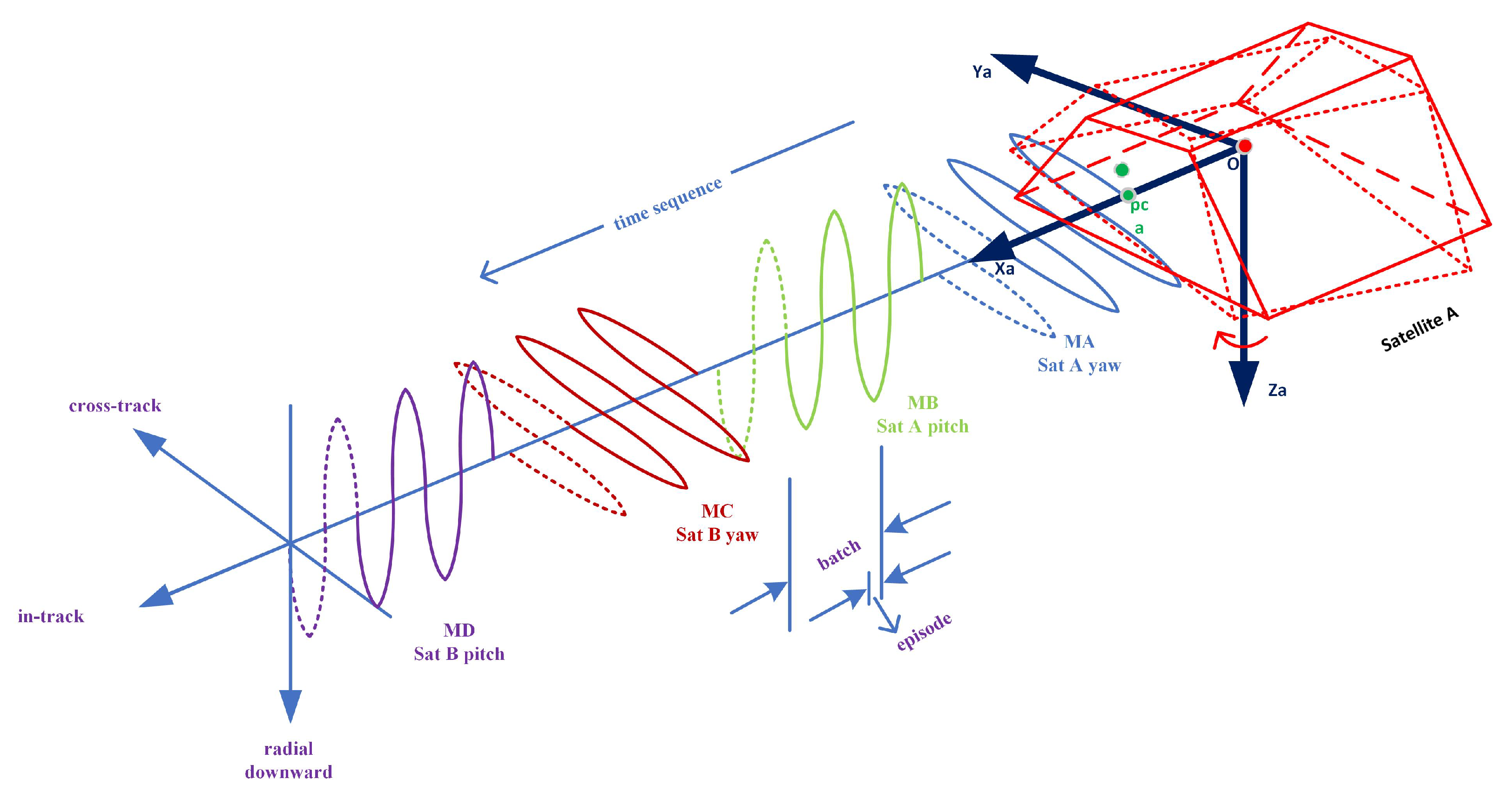
The first step to assess APC calibration performance is using software. Here we use a simple low-Earth-orbit follow-on formation scene in circular orbit with the following parameters: Satellite A orbit altitude: 470 km; inclination: 89 deg; argument of perigee: 0 deg; right ascension of ascending node (RAAN): 0 deg; true anomaly: 0 deg, and satellite B performs a follow-on flight relative to satellite A, with a distance of about 170 km in-track.

The two satellites are propagated separately in the inertial frame, using high-accuracy numerical integration, and the relative orbit information is calculated from the differences. The satellite construction model from GRACE is used for the attitude perturbations analysis in space condition [30].

The gravitational and non-gravitational accelerations used here are summarized as in

Table 1. Accelerations of gravitational and non-gravitational models.

Items *	Model
GA—the geopotential effect of the Earth	20th order and degree
GA—Sun, and Moon gravities	DE405/LE405 planetary ephemerides model
GA—solid Earth tides	IERS Conventions 1996
GA—ocean tides	Center for Space Research 3.0 model
NGA—the atmospheric drag	NRLMSISE-00 empirical model
NGA—the solar radiation pressure	IERS Standards 1992

* note: GA (gravitational accelerations), NGA (non-gravitational accelerations).

.

To fully test and verify the APC calibration accuracy in space missions, the authors have conducted APC calibration simulation (ACS) software development based on a MATLAB/Simulink environment. The core of ACS is maneuver control and RL scene, as shown in Figure 5. During ACS simulation, both GA and NGA dynamics are propagated, with periodic oscillation maneuvers of all kinds performed sequentially, as in Section 2.1, including mirror maneuvers. All the data from ACS are put together into the RL block, in which the typical RL algorithm and TDAAC algorithm can be performed with on-line/off-line maneuver parameters regulating. The final evaluation of APC calibration accuracy can be provided using synchronized script files. Note ACS can also function as a standard high-accuracy modelling software that provides preliminary Level-1B data in a 5 s sampling rate, from initial 1 January 2000, 12:00:00 GPS time [22], including onboard instrument output of GPS navigation data, MWR ranging, star camera quaternions, accelerations and Laser ranging interferometer (LRI) data [11].

4.2. ASC Simulation Using Traditional Method

Here we first provide the APC calibration results without the RL process. Suppose we known the fixed real position of APC

$${\mathbf{d}}_{pca}={\left[\begin{array}{ccc}1.4& 0.02& 0.02\end{array}\right]}^{\mathrm{T}}\mathrm{m},{\mathbf{d}}_{pcb}={\left[\begin{array}{ccc}1.4& 0.02& 0.02\end{array}\right]}^{\mathrm{T}}\mathrm{m}$$

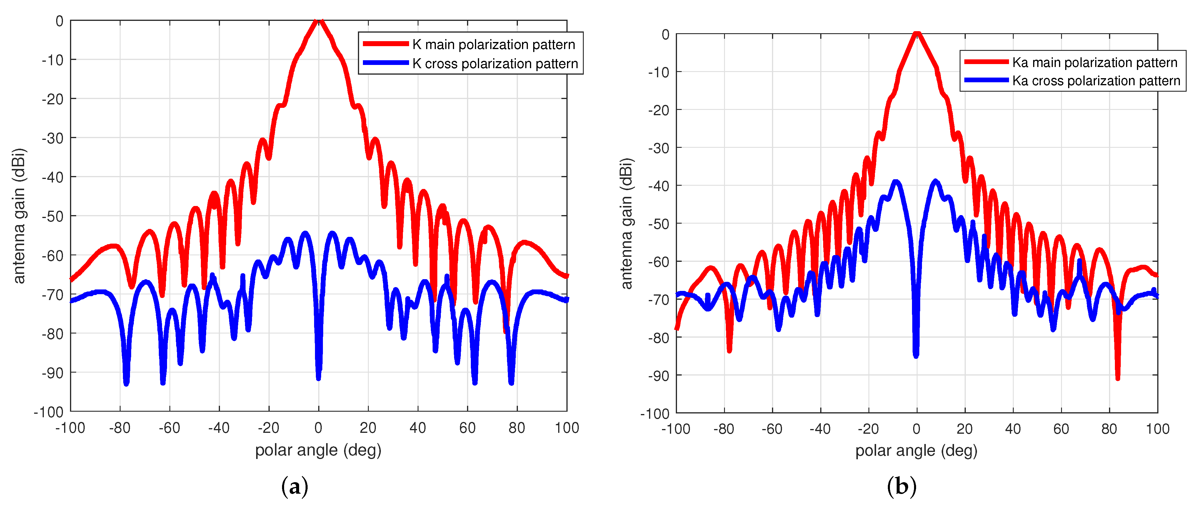
in the spacecraft frame, for both satellite A and B. The real models of K/Ka dual frequency antenna gain pattern and induced signal process noise are used. The moment of inertia for the two satellites are

$${\mathbf{I}}_a={\mathbf{I}}_b={\left[\begin{array}{ccc}80& -3& -3\\ -3& 420& -0.3\\ -3& -0.3& 470\end{array}\right]}^{\mathrm{T}}\mathrm{kg}·\mathrm{m}{}^2$$

and the attitude maneuver control is simply conducted through a PID algorithm. APC with period maneuver is used here with maximin amplitude of 1 deg in yaw direction, 3 deg in pitch direction, and the period of the oscillation is set to about 250 s. Note the period maneuver parameters are constrained by the ADCS system of the satellite platform and attitude actuators on-board.

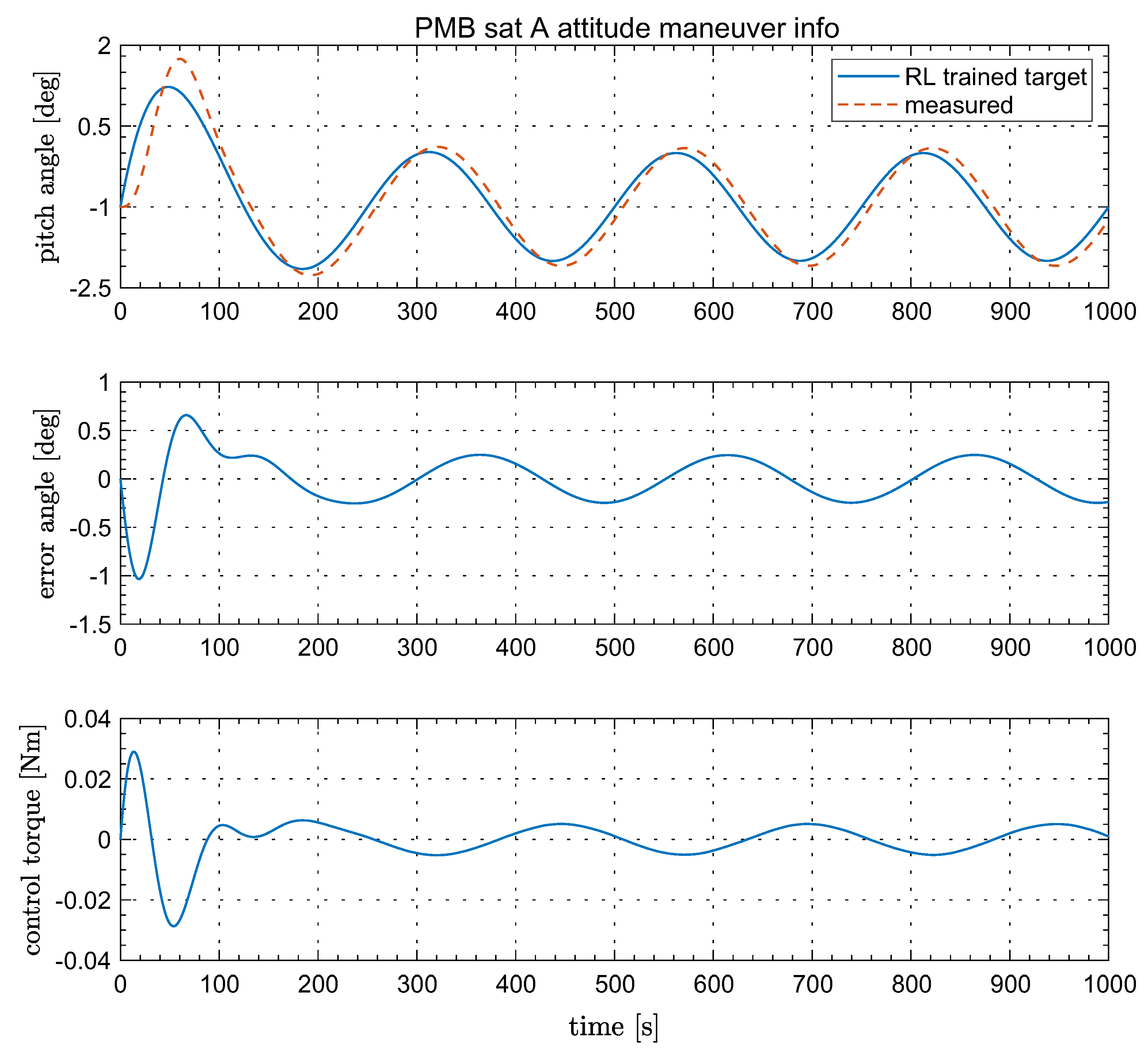
The APC calibration simulation lasted for 4000 s with 4 full sub-maneuvers, 1000 s each, and sampling time is 5 s. Figure 6 provided the simulated attitude results of satellite A, through sub-maneuver A and B in yaw and pitch directions. The data include target attitude, real attitude from measurement, attitude control error and the attitude control torque. By using the traditional APC batch algorithm, we have the final APC estimation value of

$${\widehat{\mathbf{d}}}_{pca}=\left[\begin{array}{c}1.39978115\\ 0.00999946\\ 0.00965884\end{array}\right]\mathrm{m},{\widehat{\mathbf{d}}}_{pcb}=\left[\begin{array}{c}1.39645232\\ 0.01006331\\ 0.00963114\end{array}\right]\mathrm{m}$$

With Equation (8) in Section 2.1, the APC calibration error is 0.243 mrad for sat A, 0.254 mrad for sat B.

4.3. RL Simulation Using ACS Software

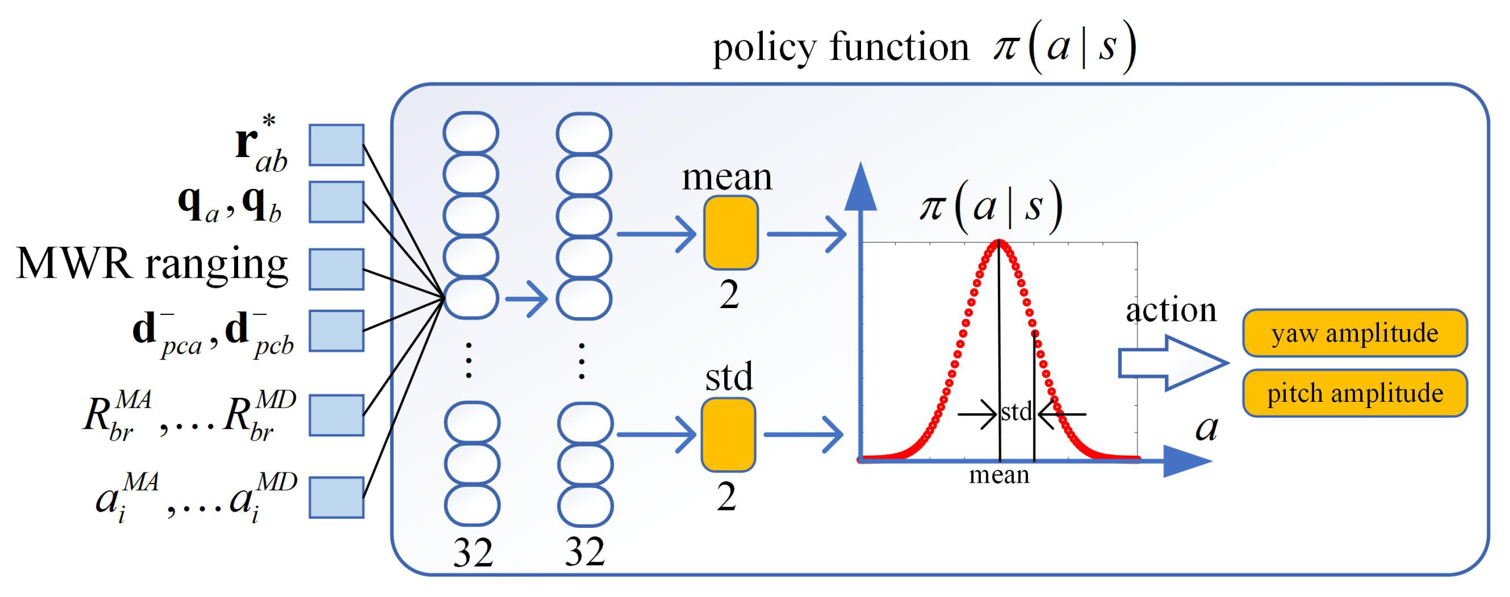
To test the APC calibration algorithm with the RL process in a software environment, here we use two neural networks that approximate the value prediction and action taken. The NN consist of input, hidden layer and output layer, while the input of both networks including measurement from carrier phase differential GPS ${\mathbf{r}}_{ab}^{*}$, attitude from star sensor ${\mathbf{q}}_a,{\mathbf{q}}_b$, and MWR ranging, and states vector, as in Section 2.1. The hidden and output layer composed of neural nodes with affine transformation and nonlinear mapping functions, as

$$a_j^{\left[i\right]}=\sigma \left({\mathbf{W}}^{\left[i\right]}{\mathbf{a}}^{\left[i-1\right]}+{\mathbf{b}}^{\left[i\right]}\right)$$

(32)

where $a_j^{\left[i\right]}$ is the output of the j-th node in i-th layer, ${\mathbf{a}}^{\left[i-1\right]}$ is the stacked output of the previous layer, ${\mathbf{W}}^{\left[i\right]},{\mathbf{b}}^{\left[i\right]}$ are the weights and biases of the i-th layer, and $\sigma \left(·\right)$ is the activation function. Here we use the critic network of 2 hidden layers of 64 nodes, with the Rectified Linear Unit (ReLU) activation function.

For the purpose of the policy function approximate, the actor NN is used with ReLU nodes in hidden layers, and a sinusoidal function for limited output layer. The final output provides the mean and standard deviation of two normal distributions for the yaw and pitch maneuvers amplitude angle in the form of a probability distribution function, and the results feedback to the ACS target quaternion block as marked ① in Figure 5. The NN diagram for the proposed RL-based APC calibration is depicted in Figure 7 and Figure 8 as

The training target is to minimize the APC estimation error from the batch algorithm, with the optimal periodic oscillation amplitude, rather than the nominal designed 1 deg around 3 deg initial bias angle in yaw maneuver. Note the K band antenna gain would decrease dramatically out of 6 deg in the main lobe, so we just need to sample actions within 3 deg from the policy, avoiding the whole action space exploration. The similar settings also apply to the pitch maneuver with 3 deg amplitude around −1 deg initial bias angle. The instant reward function is given as

$$r\left(t\right)=-\left[\begin{array}{cc}{w}_1& w_2\end{array}\right]\left[\begin{array}{c}eAn{g}_a\left(t\right)\\ eAn{g}_b\left(t\right)\end{array}\right]$$

(33)

where the definition of $eAn{g}_{a,b}\left(t\right)$ can be found in Equation (9), and $w_1,w_2$ denote reward function weights.

The final target APC estimation accuracy interval is a trade-off situation that have to be considered for RL implementation. Here we use the idea of shrinking goal interval, with 0.003 mrad decreasing for each training episode [25]. The purpose of doing this is to avoid lack of training with a quick APC calibration process finished, under a large goal interval; and also avoid low chances of reaching the goal interval through the exploration step.

The RL training episode consists of 100 steps each, with each step of 0.05 s in the ACS software. This timing sequence can be easily interpolated into an attitude control system for on-line APC maneuver execution.

Table 2. Hyperparameters used in simulation.

Hyperparameter	Value
critic network	2 hidden/64 nodes/ReLU
actor network	1 hidden/32 nodes/ReLU, 1 output/sinusoidal
discount factor	0.99
learning rate	0.001
critic weights $w^{\left[i\right]}$ and biases $b^{\left[i\right]}$	1/64, 0
actor weights $w^{\left[i\right]}$ and biases $b^{\left[i\right]}$	1/64, 0
memory buffer, $\mathcal{B}$	storage space for 10 sampling time
max iterations, L	5
actors number, N	50
Epochs, K	200
Time steps, T	100
1 episode	100 steps
learning step size	0.05 s

below provided the parameters used during simulation:

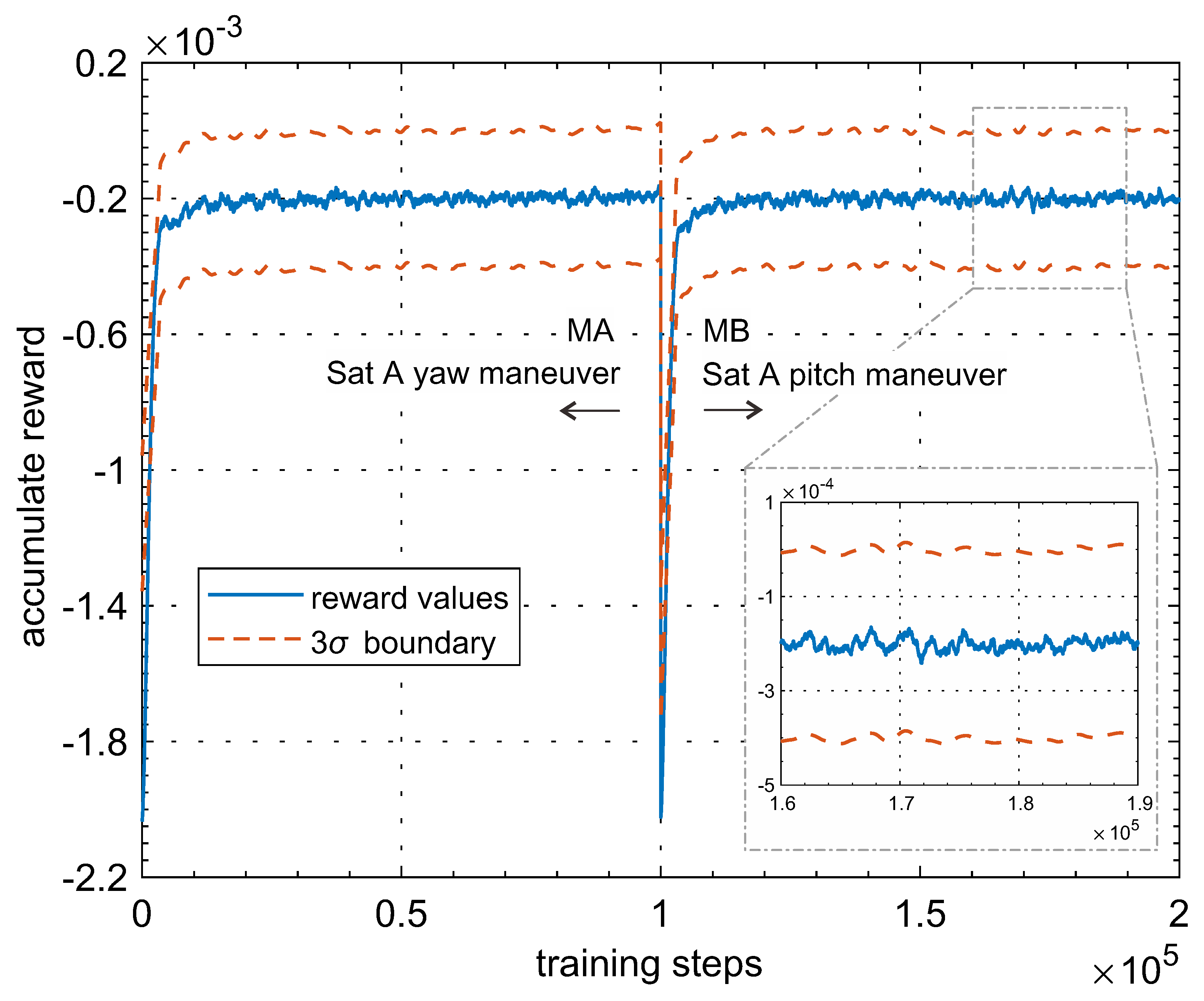
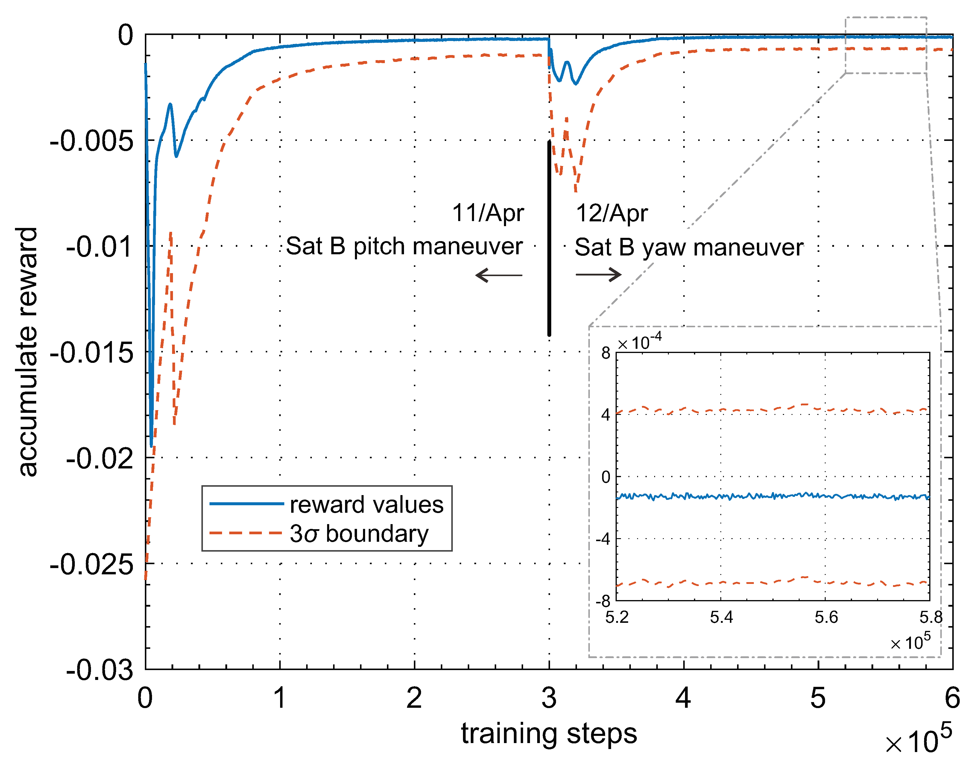
The data collected from the RL training process during APC calibration are shown in Figure 9 as a solid red line for reward and dotted green lines for deviation. Only the results of satellite A from sub-maneuvers A and B are provided here for the purpose of simplicity. We may find that the training results converged gradually to the real APC position. According to the definition of reward in Equation (9), the policy NN can be trained to steady within about 40 thousand steps, and the final APC calibration error may be below 2 mrad, as in zoom in subfigure in Figure 9, which is more accurate than the traditional batch algorithm. After the post-data statistics, we found the accumulated reward is improved from MA to MB, after the training NN converges. The reason may be explained as this: the APC position is composed of elevation and horizontal values in the antenna coordinate frame, which can be estimated through on-orbit maneuvers in yaw and pitch directions for one satellite. Surely more accuracy results may be obtained after two maneuvers. Similar results can be found for satellite B through sub-maneuvers C and D, which are not shown here.

It is interesting to explore what kind of sub-maneuvers trajectory we may obtain from the NN training process. The target attitude maneuver amplitude finally converged to about 1.1 deg for both MA and MB, in yaw and pitch direction. Figure 10 provides the MB pitch angle values with attitude control error and control torque. The trained target amplitude, not considering the constraints of satellite ADCS, is mainly affected by the emission gain of the antenna. The optimal attitude amplitude balances the APC observation sensitivity in yaw and pitch directions and the deteriorated MWR ranging error outside the antenna main-lobe.

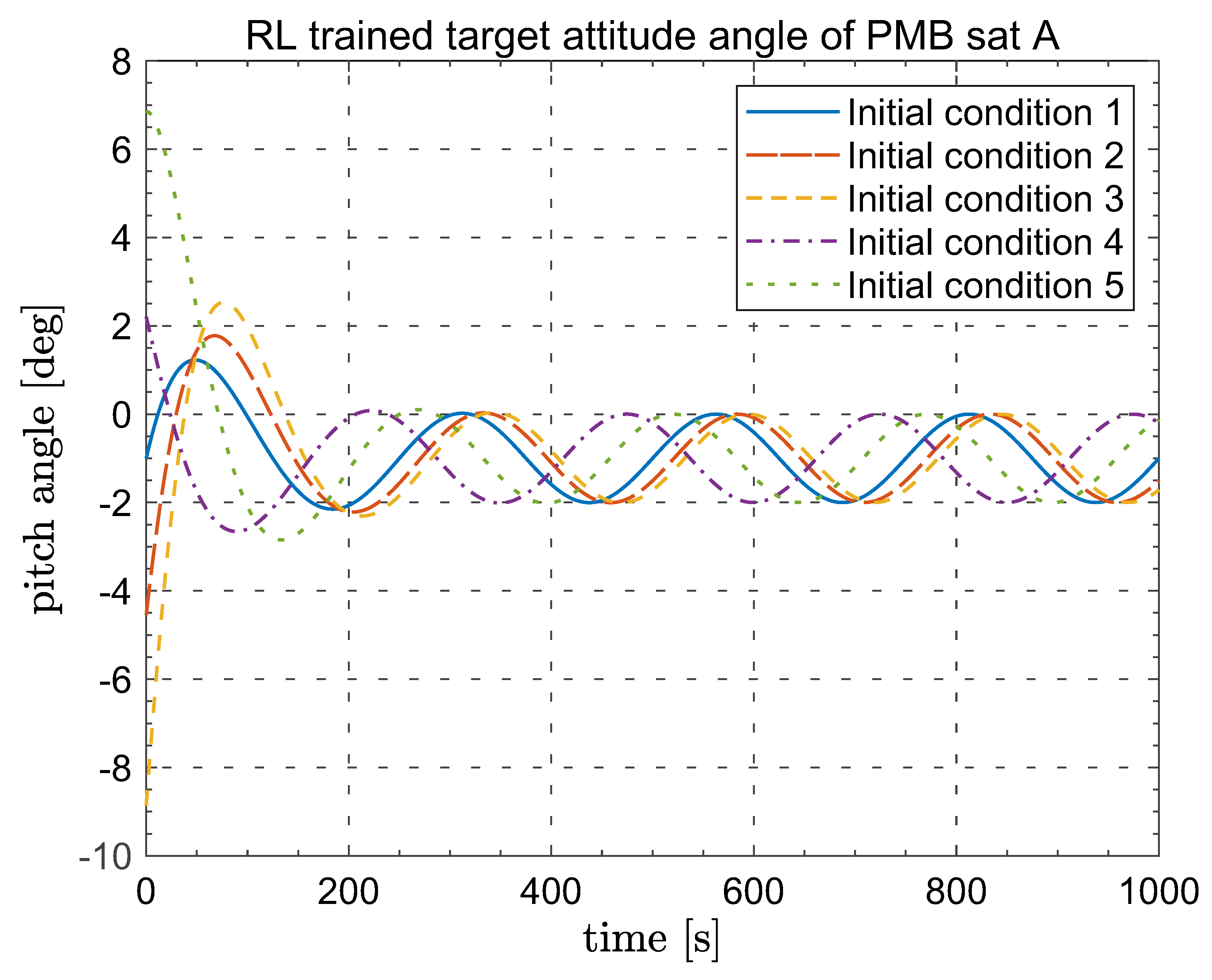
Moreover, Figure 11 provided the trained target amplitude of MB pitch angles under different initial conditions. We may find that the trained output converge quickly with the expected values as shown before, which verified the effectiveness of the proposed method.

Recall that the initial attitude angles for APC calibration are predefined as 3 deg in yaw maneuver, and −1 deg in pitch. It would be curious to find what results we may obtain if the initial angles changed. Figure 12 shows the modified policy NN with output, including both initial angles and amplitudes. The final results after simulation are as follows: initial angles around 2.8 deg in yaw and −1.5 deg in pitch, and the amplitudes converged to about 1 deg for yaw and pitch. The trained initial pitch angle, around −1.5 deg, is reasonable since the predefined −1 deg is aiming to get LOS pointing between satellite A and B on-orbit, in orbit frame, and −1.5 deg can obtain more sensitive MWR observing data for APC estimation.

RL-based APC calibration can obtain better results after training, compared with traditional batch algorithm. More importantly, the RL architecture can be extended to deep training applications such as the feedback to attitude control system, as number mark ② in Figure 5, or extended to linear calibration maneuvers with proof mass states and attitude dynamic equations. Those would be provided in the authors’ following publications.

5. Laboratory RL Test

The RL-based APC calibration simulation results in the previous section are on the basis of the known APC position in the body frame as a priori. We have to be aware that it is not true in real space flight, and the RL algorithm has to be modified to deal with this situation.

To fully explore the possible application of the RL algorithm to APC in a space environment, with real antenna onboard, the authors have conducted a hardware in loop (HIL) test on-ground, as shown in Figure 13. The experiment is performed in a near-field microwave un-reflected chamber, with a full-scale satellite structure model fixed on a high-accuracy rotation platform. Other instruments in the HIL system include microwave signal source, electronic theodolite, signal sampling and process computer.

The experiment is initially APC aligned, and holds still during the whole test process. With platform rotation, we can simulate the on-orbit attitude maneuvers for the APC algorithm. Measurement data were collected, and used for the RL training process. The simulation scene is the same as Section 4, while the only difference is the antenna azimuth angle has to be re-fixed by rotating 90 deg in the rolling axis, to simulate the different sub-maneuvers. The reason for this azimuth change is due to the constraint of only a one-dimensional rotation from platform.

Although the pre-calibrated APC information can be obtained before the HIL test, we still need to consider APC as unknown during test to simulate the situation in space, and the reward function is defined as

$$r\left(t\right)=-\left[\begin{array}{cc}{w}_3& w_4\end{array}\right]\left[\begin{array}{c}\overline{e}An{g}_a\left(t\right)\\ \overline{e}An{g}_b\left(t\right)\end{array}\right]$$

(34)

where the definition of $\overline{e}An{g}_{a,b}\left(t\right)$ can be found in Equation (10), and $w_3,w_4$ are weights.

Prior parameters of NN from a previous RL training process are used for the HIL APC calibration system, including weight and bias data sets. The trained NN program is compiled and uploaded to the HIL control system, and Figure 14 provided the results of reward values during HIL APC simulation. Obviously, we get the sharp vibrated data this time, compared with ACS simulation. The reason for this phenomenon is mainly due to the platform rotation control system, which is not smooth enough in angular rate control. However, the final trained APC calibration error can still be achieved to less than 2 mrad, as in zoomed in subfigure of Figure 14.

6. On-Orbit RL Verification

The formation satellites have successfully launched in 19:13, 29 December 2021 in Jiuquan, China, known as TianHui-4, deployed with MWR instrument onboard [31]. The main task of this space mission is fully testing the high-accuracy micrometre level ranging technology for multiple applications. Several attitude maneuvers have been performed on-orbit during 11–12 April 2022 for APC calibration, as shown in Figure 15, and traditional algorithms for APC estimation is used instantly with a calibration accuracy of less than 3 mrad for satellite B.

The authors have been deeply involved in all the stages of the MWR payload design and traditional APC calibration process. It is interesting to explore the possible use of RL to the APC calibration with different results. Several situations should be considered, compared with APC software simulation: First, the satellite attitude dynamic modeling and control is conducted by the ADCS department, affiliated with the China academy of space technology (CAST), and detailed controller parameters cannot be obtained, leading to the attitude system missing identifications. Moreover, the satellites experienced real perturbations in space, which cannot be fully duplicated in software simulation.

The structure of deployed formation satellites is a hexahedron shape prismatic, as half side shown in Figure 16 below. The length of the lower side trapezoidal section is 1900 mm, upside 700 mm, and height 750 mm. The total length of satellite is 3200 mm, weight of about 650 kg. The actuators of ADCS of both satellites include cold-gas propulsion and magnetorquer (MTQ). For most of the time, the satellite works in the three axes steady state, and the MTQs are used to compensate orbit disturbance torques with high-precision attitude control performance. The cold-gas propulsion actuator is used only for situations of large attitude maneuvers such as APC calibration on-orbit. There is a total of 12 thrusters onboard for attitude control, arranged in pairs in the opposite directions around each twin satellite platform, as shown in Figure 16, and each cold-gas thruster can provide 10 mN thrust within one continuous minute, providing more attitude control capability than MTQs.

The algorithm for the ADCS during APC calibration maneuvers on-orbit is sophisticatedly designed, by an optimal combination of cold-gas propulsion and MTQs. Since we cannot obtain the real attitude control strategy on-orbit, it is meaningful to conduct backward RL training operate, to get the critical weights and bias of NNs from real attitude maneuver data in space. The purpose of backward training is to verify the effectiveness of the RL algorithm for autonomous intelligent close-loop attitude control in near future, and evaluate the APC accuracy with the trained RL parameters on-orbit.

The backward RL training process is scheduled like this: first, the initial attitude angle and periodic oscillation amplitude in pitch and yaw directions are obtained through the least square method, from on-orbit data, as in Figure 15. We may notice that the real attitude maneuver amplitude on-orbit is less than 1 deg, unlike the previously trained 1.1 deg using ASC simulation. This is more possible to get the preliminary calibration maneuvers test on-orbit for the first time, or, just balance the APC performance and cold-gas consumption. Second, reward function of Equation (34) is used here, since no APC position is known as a priori. Next, the shrinking goal interval is still used here as before, and the episode moves forward to the next sequence if training failed to reach the goal APC accuracy. Finally, the policy NN is adjusted to output recommended actions at each step, the algorithm autonomously records the bias between action output and real amplitude.

The on-board APC maneuver data of 3000 s length is selected with 600 time points and 5 s intervals from Figure 15, for both 11 and 12 April. Figure 17 provided the collected data during RL process, with a solid red line for accumulated reward and deviation of 3 $\sigma$ boundaries. Thanks to the 3000 s long time RL duration, we may finally obtain the converged APC estimation of about 1.5 to 2 mrad accuracy in the antenna frame, as with the detailed results in zoomed in subfigure in Figure 17. Clearly, this is more effective than traditional batch algorithm, and more importantly, the RL method may be extended to a more general form with proof mass center calibration in the spacecraft body frame.

7. Discussion

According to the analysis from the software/HIL test and on-orbit data, the RL-based APC calibration method performed stably and provided high-accuracy APC estimation results, compared with the traditional method. The final APC calibration accuracy is less than 2 mrad from the on-ground test, and may achieve 1–1.5 mrad from the on-orbit training process, which fulfilled the engineering requirements. Most importantly, the RL algorithm may function fully autonomously on-orbit, which may optimally balance the APC process accuracy (value) and the attitude maneuvers (action) taken. Moreover, the proposed RL-based APC algorithm may extend to proof mass calibration scenes with actions feedback to the ADCS system, revealing flexibility of real applications to spacecraft payload system in the future.

References

1. Jun, L.U.O.; Linghao, A.I.; Yanli, A.I. A brief introduction to the TianQin project. Acta Sci. Nat. Univ. Sunyatseni 2021, 60, 1. [Google Scholar]
2. Luo, Z.; Zhang, M.; Jin, G.; Wu, Y.; Hu, W. Introduction of Chinese Space-borne Gravitational Wave Detection Program“Taiji”and “Taiji-1”Satellite Mission. J. Deep. Space Explor. 2020, 7, 3–10. (In Chinese) [Google Scholar]
3. Heinzel, G. Advanced Optical Techniques for Laser-Interferometric Gravitational-Wave Detectors; Gottfried Wilhelm Leibniz Universität Hannover: Hannover, Germany, 1999. [Google Scholar]
4. Dehne, M.; Cervantes, F.G.; Sheard, B.; Heinzel, G.; Danzmann, K. Laser interferometer for spaceborne mapping of the Earth’s gravity field. J. Phys. 2009, 154, 12023. [Google Scholar] [CrossRef]
5. Sun, H.; Sun, W.; Shen, W.; Shen, C.; Zhu, Y.; Fu, G.; Wu, S.; Cui, X.; Chen, X. Research progress of Earth’s gravity field and its application in geosciences—A summary of Annual Meeting of Chinese Geoscience Union in 2020. Adv. Earth Sci. 2021, 36, 445–460. [Google Scholar] [CrossRef]
6. Wand, V. Interferometry at Low Frequencies: Optical Phase Measurement for LISA and LISA Pathfinder. Ph.D. Thesis, Gottfried Wilhelm Leibniz Universität Hannover, Hannover, Germany, 2007. [Google Scholar]
7. Bender, P.L.; Hall, J.L.; Ye, J.; Klipstein, W.M. Satellite-satellite laser links for future gravity missions. Space Sci. Rev. 2003, 108, 377–384. [Google Scholar] [CrossRef]
8. Müller, V.; The GRACE Follow-On LRI Team. Laser Ranging Interferometer on GRACE Follow-On: Current Status//EGU General Assembly Conference Abstracts. In Proceedings of the EGU General Assembly 2020, EGU2020-10566, Online, 4–8 May 2020. [Google Scholar] [CrossRef]
9. Abich, K.; Abramovici, A.; Amparan, B.; Baatzsch, A.; Okihiro, B.B.; Barr, D.C.; Bize, M.P.; Bogan, C.; Braxmaier, C.; Burke, M.J.; et al. In-orbit performance of the GRACE follow-on laser ranging interferometer. Phys. Rev. Lett. 2019, 123, 31101. [Google Scholar] [CrossRef] [PubMed]
10. Goswami, S.; Devaraju, B.; Weigelt, M.; Mayer-Gurr, T. Analysis of GRACE range-rate residuals with focus on KBR instrument system noise. Adv. Space Res. 2018, 62, 304–316. [Google Scholar] [CrossRef]
11. Darbeheshti, N.; Wegener, H.; Müller, V.; Naeimi, M.; Heinzel, G.; Hewitson, M. Instrument data simulations for GRACE Follow-on: Observation and noise models. Earth Syst. Sci. Data 2017, 9, 833–848. [Google Scholar] [CrossRef]
12. Koch, A.; Sanjuan, J.; Gohlke, M.; Mahrdt, C.; Brause, N.; Braxmaier, C.; Heinzel, G. Line of sight calibration for the laser ranging interferometer on-board the GRACE Follow-On mission: On-ground experimental validation. Opt. Express 2018, 26, 25892–25908. [Google Scholar] [CrossRef] [PubMed]
13. Wang, F. Study on Center of Mass Calibration and K-Band Ranging System Calibration of the GRACE Mission; The University of Texas at Austin: Austin, TX, USA, 2003. [Google Scholar]
14. Sutton, R.S.; Barto, A.G. Adaptive Computation and Machine Learning Series, Reinforcement Learning: An Introduction, 2nd ed.; The MIT Press: Cambridge, MA, USA, 2018. [Google Scholar]
15. Mnih, V.; Badia, A.P.; Mirza, M.; Graves, A.; Lillicrap, T.P.; Harley, T.; Silver, D.; Kavukcuoglu, K. Asynchronous methods for deep reinforcement learning. In Proceedings of the International Conference on Machine Learning, New York, NY, USA, 19–24 June 2016; pp. 1928–1937. [Google Scholar]
16. Sutton, R.S.; McAllester, D.; Singh, S.; Mansour, Y. Policy gradient methods for reinforcement learning with function approximation. Adv. Neural Inf. Process. Syst. 1999, 12, 1057–1063. [Google Scholar]
17. Degris, T.; White, M.; Sutton, R.S. Off-policy actor-critic. arXiv 2012, arXiv:1205.4839. [Google Scholar]
18. Schulman, J.; Levine, S.; Abbeel, P.; Jordan, M.I.; Abbeel, P. Trust region policy optimization. In Proceedings of the International Conference on Machine Learning, Lille, France, 7–9 July 2015; pp. 1889–1897. [Google Scholar]
19. Khoroshylov, S.V.; Redka, M.O. Deep learning for space guidance, navigation, and control. Space Sci. Technol. 2021, 27, 38–52. [Google Scholar]
20. Izzo, D.; Märtens, M.; Pan, B. A survey on artificial intelligence trends in spacecraft guidance dynamics and control. Astrodynamics 2019, 3, 287–299. [Google Scholar] [CrossRef]
21. Ravaioli, U.J.; Cunningham, J.; McCarroll, J.; Gangal, V.; Dunlap, K.; Hobbs, K.L. Safe Reinforcement Learning Benchmark Environments for Aerospace Control Systems. In Proceedings of the 2022 IEEE Aerospace Conference (AERO), Big Sky, MT, USA, 5–12 March 2022; pp. 1–20. [Google Scholar] [CrossRef]
22. Case, K.; Kruizinga, G.; Wu, S. GRACE Level 1B Data Product User Handbook; JPL Publication D-22027; JPL: Pasadena, CA, USA, 2002. [Google Scholar]
23. Kim, J. Simulation Study of a Low-Low Satellite-to-Satellite Tracking Mission. Master’s Thesis, The University of Texas, Austin, TX, USA, 2000. [Google Scholar]
24. Wang, X.; Gong, D.; Jiang, Y.; Mo, Q.; Kang, Z.; Shen, Q.; Wu, S.; Wang, D. A Submillimeter-Level Relative Navigation Technology for Spacecraft Formation Flying in Highly Elliptical Orbit. Sensors 2020, 20, 6524. [Google Scholar] [CrossRef] [PubMed]
25. Pi, C.H.; Hu, K.C.; Cheng, S.; Wu, I.-C. Low-level autonomous control and tracking of quadrotor using reinforcement learning. Control. Eng. Pract. 2020, 95, 104222. [Google Scholar] [CrossRef]
26. Sutton, R.S.; Barto, A.G. Reinforcement Learning: An Introduction; MIT Press: Cambridge, MA, USA, 1998; p. 22447. [Google Scholar]
27. Schulman, J.; Wolski, F.; Dhariwal, P.; Radford, A.; Kilmov, O. Proximal policy optimization algorithms. arXiv 2017, arXiv:1707.06347. [Google Scholar]
28. Sutton, R.S. Learning to predict by the methods of temporal differences. Mach. Learn. 1988, 3, 9–44. [Google Scholar] [CrossRef]
29. Munos, R.; Stepleton, T.; Harutyunyan, A.; Bellemare, M. Safe and efficient off-policy reinforcement learning. In Proceedings of the 30th International Conference on Neural Information Processing Systems, Barcelona, Spain, 5–10 December 2016. [Google Scholar]
30. Bettadpur, S. Gravity Recovery and Climate Experiment: Product Specification Document; GRACE 327-720; CSR-GR-03-02; Center for Space Research, The University of Texas at Austin: Austin, TX, USA, 2012. [Google Scholar]
31. Available online: http://finance.people.com.cn/n1/2021/1229/c1004-32320072.html (accessed on 29 December 2021).
Figure 1. Illustration of sub-maneuver A (MA) for APC calibration, a small positive yaw angle maneuver is performed for satellite A.
Mathematics 11 00942 g001
Figure 2. MWR antenna design with prototype. (a) MWR antenna design. (b) Prototype of MWR antennas for satellites A and B.
Mathematics 11 00942 g002
Figure 3. K/Ka antenna main polarization and cross polarization pattern. (a) K antenna. (b) Ka antenna.
Mathematics 11 00942 g003
Figure 4. Illustration of training process during sub-maneuvers. (MA means sub-maneuver A).
Mathematics 11 00942 g004
Figure 5. SIMULINK block diagram for APC calibration simulation.
Mathematics 11 00942 g005
Figure 6. Software simulation of APC calibration maneuver (MA & MB). (a) Satellite A yaw maneuver information. (b) Satellite A pitch maneuver information.
Mathematics 11 00942 g006
Figure 7. Schematic diagram of critic network.
Mathematics 11 00942 g007
Figure 8. Schematic diagram of actor network.
Mathematics 11 00942 g008
Figure 9. Learning data for software APC calibration simulation.
Mathematics 11 00942 g009
Figure 10. Satellite A pitch maneuver attitude information during software APC calibration simulation.
Mathematics 11 00942 g010
Figure 11. Satellite A pitch maneuver angles under different initial conditions.
Mathematics 11 00942 g011
Figure 12. Schematic diagram of extended output policy network.
Mathematics 11 00942 g012
Figure 13. RL-based APC calibration in laboratory HIL environment.
Mathematics 11 00942 g013
Figure 14. Learning data for laboratory HIL APC calibration simulation.
Mathematics 11 00942 g014
Figure 15. On-orbit attitude maneuvers for APC calibration during 11–12 April 2022. (a) Satellite B pitch maneuver. (b) Satellite B yaw maneuver.
Mathematics 11 00942 g015
Figure 16. Illustration of cold-gas thrusters arrangement in body frame.
Mathematics 11 00942 g016
Figure 17. Learning data for on-orbit APC calibration during 11/12 Apr.
Mathematics 11 00942 g017