1. Introduction
There have been a number of developments in searching for the stability criteria for nonlinear delay differential systems, but most of these have been restricted to finding asymptotic stability conditions.
As noted in [
1], this may be caused by the fact that ‘a “geometric” view of nonlinear dynamics leads one to adopt the view that notions of stability should be invariant under (nonlinear) changes of variables’. For this reason, ‘exponential stability is not a natural mathematical notion when nonlinear coordinate changes are allowed. This is why the notion of asymptotic stability is important’ [
1].
However, in some cases it is necessary not only to establish the fact of asymptotic stability, but also to know the rate of convergence in the asymptotic stability property—for example, in order to guarantee some asymptotic properties of solutions to a cascaded system based on an analysis of the properties of its isolated subsystems [
1]. In practical applications, it is also important to guarantee a certain rate of convergence of some characteristics of the system.
At the same time, the exponential stability of nonlinear systems is not easily verified. Moreover, for systems with delay, even in the linear case, there are difficulties in estimating the rate of convergence of solutions (see, for example, references in [
2]).
Therefore, researchers are attracted by the problem of obtaining requirements for the Lyapunov function, which can guarantee estimates for the convergence of solutions.
The specificity of using finite-dimensional functions to analyze the stability properties of systems with delay is that the derivative of the Lyapunov function is estimated not in the entire neighborhood of the origin, but only within its part.
The idea of such a modification of the requirements for the derivative was simultaneously proposed by N.N. Krasovskii and B.S. Razumikhin [
3,
4]. Subsequently, the conditions that determine a part of the neighborhood of zero for estimating the derivative were called Razumikhin conditions.
On one hand, these conditions simplify the practical verification of the relevant requirements that guarantee one type of stability or another. On the other hand, the absence of an estimate for the derivative of the Lyapunov–Razumikhin function along the entire solution makes it difficult to estimate the rate of decrease of the function itself, and, consequently, the estimate of the rate of convergence of solutions.
Therefore, for equations with delay, such estimates are mainly obtained using the Lyapunov–Krasovskii functionals [
5,
6]. Similar results using the functions instead the functionals have occurred from time to time and have become more frequent in the last decade; in this case, mainly autonomous or linear equations are considered (see, e.g., references in [
7]).
The purpose of this paper is to establish sufficient conditions for the exponential stability of nonlinear time-varying delay differential systems, under less restrictive assumptions on the Lyapunov–Razumikhin function (the function below) than those made in the literature so far.
Namely, the time-derivative of the constructed Razumikhin function is allowed to be neither sign-definite (as in the classical asymptotic stability theorem) nor semidefinite (as in some more general theorems, see e.g., [
8]). Moreover, a new upper estimate on the rate of decreasing of the function is obtained.
It is important to note that, in this paper, consideration is given only to deterministic systems. Nowadays, practical control systems need to meet several important requirements, for example, time delays, stochastic perturbations, time-varying parameters, and impulse effects. The research problem of stability analysis for related systems has received a great deal of attention.
The Lyapunov–Razumikhin method was originally developed to study the stability of deterministic systems with delay. However, the Razumikhin technique has also been a powerful and effective method for investigating the stability of other types of delay systems. In 1996, X. Mao extended the technique to stochastic functional differential equations to investigate
p-th moment exponential stability [
9]. In the past several decades, a large number of works on this topic have been reported in the literature (e.g., [
10,
11,
12]).
In particular, several novel criteria of the moment exponential stability are derived for the related systems; see, for example, [
13,
14,
15,
16] and references therein.
An analysis of these results shows that Razumikhin-type theorems for deterministic systems can be appropriately developed and extended to stochastic delay systems with additional features and effects. Taking into account the behavior of a specific system leads to using special tools and adding certain conditions to ensure stability. Therefore, when studying a system of a certain type, it is easier to rely on results for deterministic systems than to derive stability conditions from the available results for systems of another type. Therefore, the development of the Razumikhin method for deterministic continuous systems plays an important role both in theory and applications.
The paper is organized as follows. In
Section 2, we introduce notation, definitions, and other preliminaries.
Section 3 gives new sufficient conditions for uniform asymptotic stability and uniform exponential stability in terms of the Lyapunov–Razumikhin functions.
Section 4 contains a remark on necessary conditions for uniform asymptotic stability, which are relevant to the results obtained. In
Section 5, we consider scalar linear time-varying equations and show the effectiveness of the exponential stability theorem using some particular examples. Some more examples of nonlinear equations are given in
Section 6.
Section 7 discusses some known related results. Concluding remarks are given in the final section.
2. Preliminaries
The following notation will be used throughout the paper: is the set of all non-negative real numbers; is the n-dimensional vector space and is a norm of a vector ; time delay is denoted by r (), ; denotes the n-dimensional space of vectors with the norm ; is the Banach space with the supremum-norm . For a continuous function (, ) an element is defined for any by , , and stands for the right-hand derivative.
Consider the nonlinear system described by a time-varying delay differential equation of the form:
where
,
is a given nonlinear function satisfying
for all
. Then (
1) admits the zero solution.
In the following, we assume that the Carathéodory-type conditions from [
17] are imposed on Equation (
1). We denote the solution of (
1) with initial conditions
and
by
.
In addition, we use the following standard definition:
Definition 1. The zero solution of (1) is said to be uniformly exponentially stable (UES) if there exist constants Δ, δ, and r such that We say that the zero solution is globally uniformly exponentially stable (GUES) if .
From now on, to shorten expressions, instead of saying the zero solution of the equation is GUES, we say that the equation is GUES.
We also use the well-known concepts of uniform asymptotic stability (UAS) and global uniform asymptotic stability (GUAS).
Let
be a given function. Now, let
be a solution of (
1) starting from
, and denote by
the upper right-hand derivative of
[
18]:
Suppose that
is locally Lipschitzian in
x (uniformly in
). Then, the derivative (
2) is bounded and is equal to the upper Dini derivative of
(along the trajectory of (
1)):
where
is the right-hand side function of (
1).
Obviously, a continuously differentiable function satisfies the equality
In the sequel, we assume that is continuous in t and locally Lipschitzian in x (uniformly in t).
We also define the class of functions , is continuous, strictly increasing, and . A class- function is a function which is unbounded.
As is known, the idea that made it possible to obtain constructive results on stability in terms of functions for systems with delays was that it is sufficient to check the sign of the derivative
at each time not on the whole set
C, but only on its subset [
3,
4]. As a rule, one of two sets is used:
where
is such that
for
.
The following Razumikhin-type result of N.N. Krasovskii became the basis for further studies of the asymptotic stability of delay systems in terms of functions.
Theorem 1. Suppose that there is a function such that:
;
if and then ;
for some functions .
Then Equation (1) is UAS. It can be proved in the standard way that if , then the uniform asymptotic stability will be global (GUAS).
3. Main Result
First, we prove the following lemma, which provides an upper bound for the behavior of the function
along solutions of Equation (
1).
Lemma 1. Suppose that there exist numbers , , and the functions , , and , such that the following conditions are met:
for all and the following inequalities hold;
for :
whenever and .
Then, for any solution of Equation (1) and for all the estimation is valid with .
Proof. We define the function
along an arbitrary solution
, and the function
. It is clear that
. We define
. Then,
, while
for
, and
for
. So we have
. Notice that
. On the other hand,
and for all
we have
Then, item 3 of the theorem implies . The obtained contradiction proves that , which was to be proved. □
Based on the lemma just proved, it is easy to obtain the following result:
Theorem 2. In addition to the conditions of Lemma 1, suppose that for some , and for all , we have the estimate Then, for an arbitrary solution of Equation (1) and for all , there holds with .
In addition:
if () then Equation (1) is asymptotically stable; if () then Equation (1) is UAS; if (), and there exist constants , and such that and , then Equation (1) is UES.
Proof. Indeed, it follows from the additional condition that for the inequality is valid. Thus, we can immediately get the required estimate for .
Then, item 1 implies , and item 2 implies . The assertions of items 1 and 2 follow directly from these estimates.
It remains to prove item 3. We define the function
along an arbitrary solution
. Note that the resulting estimate for
V implies
for every
and a sufficiently large value
. Therefore,
and
. Further, take an arbitrary
and, following the idea of the proof from [
19], denote by
N the lower integer part of
. Then
, and
. Moreover, the inequality
implies
. Thus,
, where
. This implies the last assertion of the theorem. □
Remark 1. If we replace by in the conditions of items 1–3, then we obtain the conditions for global uniform asymptotic (exponential) stability.
Remark 2. It is easy to see that the condition implieswith , . In this case, , hence the second inequality in item 3 holds for an arbitrary (it suffices to put ). Moreover, for . Remark 3. Recall the definition of GUAS [1], which qualifies the speed of convergence in the GUAS property, and serves to relax exponential stability (here we modify it according to the type of equation considered). We say that the zero solution to the Equation (1) is GUAS for a given if there exists a class- function a and a positive constant so that holds for all (recall that GUAS is always equivalent to the existence of some a and like this.) We see that due to the exponential estimate for , item 2 of Theorem 2 actually implies GUAS(). Corollary 1. Let the conditions of Theorem 2 hold for . Then all statements remain true.
Proof. For the proof, we use the assumptions on the right-hand side of Equation (
1) and results from [
17].
By Assumption 2 from [
17], for each compact
there exists a locally Lebesgue-integrable function
and
such that for all
and
the estimate
holds, and
. In addition, for an arbitrary
every solution
of Equation (
1) is contained in some compact
as long as
[
17].
Now, let
be an arbitrary solution of (
1). It is clear that it suffices to check the case
. If
then
The Grönwall–Bellman inequality now implies
It remains to note that inequality will be satisfied whenever . □
Remark 4. Note that if (), then the estimate for the derivative in Theorem 2 can be replaced by the following one: for all and , where . Indeed, in this case we set , where Λ is some positive definite proper function such that . Then, the function U satisfies the conditions of Lemma 1.
4. A Remark on Necessary Conditions for Uniform Asymptotic Stability
In this section, the discussion will center on the integral conditions for the function that ensure the exponential convergence of the function to zero (Theorem 2). In fact, these conditions are equivalent to a restriction on the antiderivative of , which naturally arises in the analysis of linear ordinary differential equations with time-varying coefficients. Here, we give a statement showing that, in the nonlinear case, a similar estimate for the right-hand side is a necessary condition for uniform asymptotic stability.
Note that the requirements imposed on integrals of
to be bounded from below, which are specified in Theorem 2, are equivalent to the following condition (see [
20]):
and (
3) is equivalent to GUES for the scalar ordinary differential equation
.
Moreover, for GUES of the linear system
with a symmetric positive semidefinite matrix
, it is necessary and sufficient that (
3) be satisfied for
and every unit vector
[
21].
If the inequality
is violated, then the estimate (
3) provides sufficient GUES conditions via a quadratic time-varying Lyapunov function [
20]. Note that for a linear system, GUAS and GUES are equivalent.
Z. Artstein ([
22] Theorem 6.2) showed that the growth condition (
3) is necessary in a very general situation for ordinary differential equations. There holds a similar statement for Equation (
1):
Theorem 3. Suppose that Equation (1) is uniformly stable. Then, the equation is uniformly asymptotically stable only if there exists a compact neighborhood of zero such that for every there are numbers and b such thatfor every , and every such that , , and . Proof. Assumptions about the right-hand side of Equation (
1) ensure the positive precompactness of (
1) in an appropriate function space and the existence of the so-called limiting equations; in addition, for every limiting equation and every pair
the initial-value problem has a unique solution [
23].
Using the relationships of uniform asymptotic stability of Equation (
1) and stability properties of the corresponding limiting equations ([
23] Theorem 6), we can now repeat the proof of Theorem 6.2 from [
22] with slight modifications. □
It should be emphasized that the necessary condition for UAS from Theorem 3 without additional assumptions is not sufficient, even for ordinary differential equations ([
22] Theorem 6.3) (see also
Section 5).
5. Application: Scalar Linear Time-Varying Equations
In this section, we consider the scalar linear differential equation
where
,
, and
are piecewise continuous,
.
Note that by Theorem 3, the uniform asymptotic stability of the Equation (
4) implies the condition
for every
,
, and some numbers
and
.
There have been a lot of investigations concerning sufficient stability conditions for Equation (
4).
Most of the results obtained in this line of study impose restrictions on the sign of coefficients. For example, by Theorem 1, an Equation (
4) is uniformly asymptotically stable if
for some
and
; it is also clear that for GUES of Equation (
4), it is sufficient for the function
to satisfy the conditions of Theorem 2. In both cases, an arbitrary (bounded) delay is allowed. Moreover, if no restrictions are imposed on the delay, then for constant coefficients, the condition is the best possible.
For Equation (
4) with time-varying
a and
b as well as with a time-varying delay, sufficient GUES conditions can be refined through information about the nature of the delay variation. However, in this case, the conditions known so far usually also imply that some function depending on
a,
b, and
must retain its sign (at least for large values of
t); see [
24,
25] and references therein.
Note that the effect of delay variation can have a decisive influence on the stability even for Equation (
4) with constant coefficients: one can give an example such that for each fixed member of the range of the delay function, the associated autonomous equation is exponentially stable, yet the time-varying equation considered is unstable [
26]. However, the exact form of the relation “delay–time” is usually unknown; thus, in practice, it is more convenient to check the conditions that are valid for all delay values from a given range.
Equation (
4) with
has a separate and even richer history of study going back to the work of Myshkis (see e.g., [
27]), and this study is still ongoing. Following A.D. Myshkis, various forms of the so-called “3/2-criterion” were obtained, which establish an upper bound either for the coefficient
or for the integral of it; see some discussion and references in [
28,
29]. However, in those results, the lower bound for
(at least for the limit as
t tends to infinity) remains zero.
In [
30], the assertion is proved that if the equation
is GUES and a certain additional integral condition for
is satisfied, then Equation (
7) is GUES.
Note that the equation
is GUES if and only if (
3) hold for
(see
Section 4), while for the equation
this condition is not sufficient and additional upper bounds are required. For example, even for constant values
and
the equation
is GUAS only if
; for time-varying non-negative functions
and
, this condition turns into restrictions imposed on their supremum or some integral (see, e.g., [
27]).
But even such conditions stop working as soon as the coefficient
is allowed to change sign. The authors of [
25] investigate whether sufficiently small bounds
r for the delay and
for the integral
and exponential stability of
cause exponential stability of the equation
with an oscillating coefficient
. They provide an example showing that, unlike the case of the equation with
, such
r and
cannot be found in the general case.
Thus, the study of the stability of linear delay equations with sign-changing coefficients is a rather challenging problem. Even for the scalar Equation (
4) there are only a few results of this kind; see [
25] and references therein.
Next, we deduce sufficient GUES conditions for several examples of Equation (
4) using Theorem 2, and compare the conditions with those obtained by some other methods.
Example 1. Consider the scalar equationwith . The classical theorem (Theorem 1) implies GUAS of (1) for ; the same inequality follows from other results (see, e.g., [24] and references therein). Let be a periodic function of period 1 given bywhere and . For the derivative of the function by virtue of the Equation (1) for (), we obtain the estimate from Lemma 1 with . If , then , and if with integer , then . For , we get . Then, by Theorem 2 the conditions , are sufficient for GUES of Equation (1). In Table 1 we compare the results for Equation (1) obtained using various assertions. Note that the conditions of GUAS from [32] follow from the estimates obtained using Theorem 2. Thus, the number d can be large enough, provided that c and r are small enough. A comparison of the conditions for r, c, and d shows that for large values of r, Theorem 2 gives more restrictive conditions than [33], and vice versa for small ones. Example 2. Consider the scalar equationwith a bounded and a time-varying delay . Using the function , we find that the estimation in condition 3 of Lemma 1 holds for , where and . We denote , then and . Moreover, in condition 1 of Lemma 1, the number can be chosen to be equal to . Thus, if the zero solution of the equation is GUES, then the GUES of Equation (7) is guaranteed for sufficiently small values of r (at least for . To compare known GUES conditions with the conditions of Theorem 2, consider a special case of Equation (7) (see ([30] Example 2) and ([25] Example 4)) with the functionwhere , , and . For (7), (8) with a constant delay, the condition of GUES is obtained in the formin [30], and in the formin [25]. From Theorem 2, we get the conditions and . Table 2 lists some numerical values of the parameters α, β, and r and indicates whether the conditions of Theorem 2 or Equations (9) or (10) are satisfied for these sets. Comparing the results for Equation (8) with given by (9), we observe that the conditions do not follow from each other and may or may not be satisfied depending on the parameter values. In addition, the conditions obtained using Theorem 2 remain applicable in the case of variable delay, including a state-dependent one. Note that all the mentioned stability conditions are sufficient. Not every pair of conditions can be compared; one or the other may win, depending on the particular equation. However, it is worth noting that the previously obtained results discussed in this section were obtained using methods that make significant use of linearity of the equation under study. The results of this paper are obtained on the basis of Lyapunov–Razumikhin functions and are applicable to more general time-varying equations (see
Section 6 for some examples of nonlinear equations).
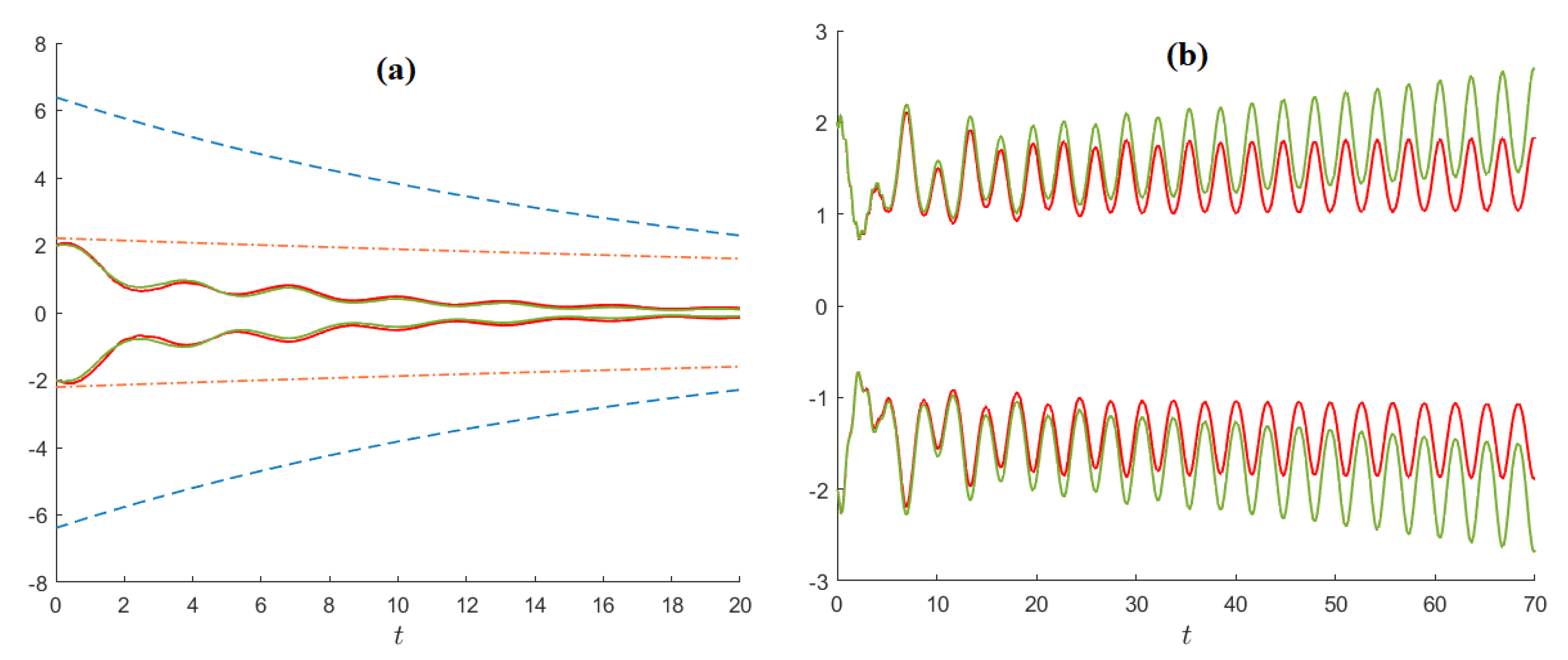
Example 3. We study the stability conditions for this equation with arbitrary values of and . For , the necessary condition GUES of the Equation (11) does not hold for . Numerical experiments show that the solutions of Equation (11) for increase indefinitely for all . Using the function , we find that the estimation in condition 3 of Lemma 1 holds for , and the conditions of Theorem 2 are satisfied for Equation (11) whenever and . In this case, for all solutions of the equation, the estimate is valid with . The given GUES conditions are satisfied, for example, for , , , , and . It can also be noted that none of the GUES conditions given in [24,25] are not applicable here. From Figure 1, we find that Equation (11) is GUES with the decay rate guaranteed by our conditions: for the selected parameter values, the norm is less than . The above GUES conditions remain valid for the equation with and for all (see an example with in Figure 1a). For comparison, the time evolutions of other functions that estimate the decay rate of solutions are also shown. These functions are calculated using formulas from ([33] Theorem 1). It is clearly seen that our estimate of M is very conservative and much worse than the estimate by [33], but the decay rate estimate gives a better result ( versus ). We also see that for the solutions of Equation (11) diverge (Figure 1b). 6. Nonlinear Examples
Example 4. Consider the systemwhere , and suppose that for some the inequality implies and for all . Using the function , we obtain that system (12) is UES whenever satisfies the conditions of Theorem 2 for some . It should be pointed out that the idea of generalizing “linear” results to a certain class of nonlinear systems using the direct Lyapunov method is used quite often; see e.g., [
29].
Example 5. Let , and be continuous and locally Lipschitz uniformly in t and take non-negative values for non-negative φ (). Define , , and , and consider the systemarising in models of population dynamics [34]. It is also assumed that takes non-negative values and there exist matrices () such that with , for [34]. Let us denote . In [34], the exponential convergence of positive solutions of (13) is proved under the condition that is a nonsingular M-matrix. Let us use the function . Estimating the derivative of this function by virtue of system (13) and applying Theorem 2 with a constant (see also Theorem 4 below), we obtain a sufficient condition for the exponential convergence of positive solutions of (13) in the form: Notice that whenever all , which corresponds to most specific models, condition (14) means that the matrix is strictly diagonally dominant. This implies that is a nonsingular M-matrix [35]. It is easy to see how, for system (13) with time-varying parameters, condition (14) can be generalized using Theorem 2. 7. Discussion
On one hand, Razumikhin’s conditions simplify the practical checking of the corresponding requirements that guarantee one type of stability or another, since the resulting estimate of the derivative does not depend on the history of the system; this circumstance, in turn, gives more "freedom” for delay in comparison with the method of functionals. On the other hand, the absence of an estimate for the derivative of the Lyapunov function along the entire solution makes it difficult to estimate the rate of convergence of solutions.
To obtain an estimate for the convergence of solutions based on Theorem 1, one can use a special structure of the time-dependent Lyapunov function, so that the convergence to zero of the function itself implies a certain rate of convergence of solutions (see, for example, [
36]).
Another approach is to modify the requirements for the function
. A significant number of modifications of Razumikhin-type theorems are based on ideas representing the so-called comparison principle. Two types of comparison theorems [
37] give rise to two types of sufficient stability conditions.
In the first case, the estimate of the derivative is constructed over the entire domain, and therefore, it has the form of a functional. Accordingly, the comparison equation is a delay equation. In the second case, the derivative of the function
is estimated over some set in the spirit of Razumikhin’s conditions, but to determine this set, it is necessary to know the solutions of the comparison equation [
37]. In the first case, to apply the result, it is necessary to obtain information about the properties of solutions of some delay equation; in the second one, it is necessary to find a solution to a (nonlinear) ordinary differential equation.
Therefore, it is natural to try to obtain more specific forms both for estimates of the derivative of the function and for Razumikhin-type conditions. The particular form of the proposed comparison equations makes it possible to obtain more constructive requirements that provide suitable properties for the solutions of these equations and, at the same time, do not lead to the "trivial” stability conditions that follow from the classical theorems. In this case, the requirements for the Lyapunov function are easier to check in specific applications, and sometimes it is also possible to obtain information about the convergence of solutions.
The results which do not make use of any Razumikhin conditions, but use a functional as an estimate of the derivative, mainly go back to the following statement:
Lemma 2 (Halanay’s lemma, [
38]).
Let be a piecewise non-negative valued function that admits constants , such that holds for all . Then, the inequality holds for all with be the root of the equation . There are a number of extensions of Halanay’s lemma to the time-varying case; they are formulated in different forms and under different assumptions, depending, among other things, on the purpose of use (e.g., [
31,
32,
39,
40,
41]). Moreover, in a number of cases, the proposed conditions imply classical requirements for the Lyapunov–Razumikhin function, which ensure (asymptotic) stability.
The requirements on the derivative in such results are relaxed due to the fact that the proposed conditions do not impose restrictions on the values of the system parameters themselves, such as delay and norms of the system coefficients, but instead involve integration of the time-varying parameters.
The second approach, which is based on the use of Razumikhin’s conditions, uses the following result in most cases:
Theorem 4. Suppose that there exists a function , numbers and , and functions such that , and whenever and . Then, along any solution of (1), the following inequalityholds for all . If, in addition, for some integer , then Equation (1) is GUES. This statement is proved in various ways and used in a number of papers (see [
7] and references therein). Some estimates for the convergence of the function
along solutions use other Razumikhin-type conditions. For discussion of a number of such results, see [
8]. Note that, in such statements, the estimate of the derivative of a (non-negative) function
is usually non-positive on the entire time interval. The question arises whether it is possible to allow the sign of the estimate of the derivative to change, and at the same time to ensure the (asymptotic) stability of the zero solution of this equation.
One of the main ideas to combine these requirements is to use integral constraints on the parameters of the system studied (including the delay). As a result, it turns out that a delay system can be asymptotically stable even if the system is described by an equation with an unstable zero solution on some (short) time intervals. Therefore, a “classical” function for such a system cannot exist.
The first result allowing usage of an indefinite time-derivative of the function
under a Razumikhin-type condition was probably given in [
42]: sufficient conditions for uniform stability are justified therein, provided that on the set
the estimate
is valid, where
, and for uniform asymptotic stability, the estimate
is additionally required for some
and sufficiently large values of
t. It is clear that such a function
does not have to be negative all the time. On the other hand, the conditions of [
42] cannot be satisfied if, for example,
is periodic and
for all
t from
where
T is the period and
. For such functions
in (
15), sufficient conditions for uniform asymptotic stability and exponential stability were obtained in [
33]: inequality (
15) should be verified on the set
, wherein the functions
and
are linked by a certain relation. Note that Theorem 2 implies Theorem 4 for
.
The results obtained here are close to the Razumikhin-type asymptotic stability theorem from [
33], but another approach is used and other exponential stability conditions are obtained. It should be mentioned at this point that in [
33] the estimate of the decay rate of solutions decreases with increasing delay, while in the estimate of Theorem 2 an increase in delay can lead to an increase in the number
M. Thus, the results of [
33] and Theorem 2 complement each other.
8. Conclusions
This paper has dealt with the problem of uniform exponential stability for nonlinear time-varying delay systems. We apply the Razumikhin method to establish sufficient conditions for exponential stability, and propose an extension of the Razumikhin approach for time-varying systems. Namely, the time-derivative of the constructed Razumikhin function is allowed to be indefinite, and a new upper estimate on the rate of decreasing of the function is also obtained.
The statements deduced can be seen as extensions of those in some earlier work discussed in the previous section, as well as some known sufficient conditions for the exponential stability of linear delay equations. The application of the exponential stability conditions derived here to specific examples shows that the previous related results are either inapplicable or give some other exponential estimates for the solutions.
We note that the use of the Razumikhin method gives rise to stability conditions that are sufficient but not necessary. Therefore, such stability conditions may be overly conservative. Various approaches have been taken to reduce the conservatism of the method, and numerous results have been obtained in this area. However, no universally good stability criterion exists; which criterion is better depends on what a specific system is.
The simple examples given in the paper show that Theorem 2 can be less conservative than other methods.
The method used in this paper for estimating the function
V along solutions of a differential equation can be extended to wider classes of differential equations. It can also be used to solve other problems. For example, in [
39], similar estimates are used for sufficient conditions for practical stability (exponential stability is a special case; see ([
39] Remark 1)). Parenthetically, in [
39] the coefficient of
V in the estimate of the derivative is negative.
In [
16], methods from [
33] are extended to stochastic systems, as well as to studying other types of stability, in particular input-to-state stability and integral input-to-state stability. In [
14], the ideas of [
33] were developed for impulsive stochastic systems with delay. For such systems, it is necessary not only to construct estimates for a function
V on continuity intervals, but also to take into account the change in this function at impulse moments. The most important feature of the results from [
14] is that time-derivatives of Razumikhin functions are allowed to be unbounded.
We also note the recent work [
43], in which the reaction–diffusion epidemic model with a delayed impulse is studied. For this model, a new synchronization criterion is obtained. In this case, the Lyapunov–Krasovskii functional is used, but the estimate for the derivative also has the form
with
.
Therefore, the results obtained in this paper can be extended both to other types of equations and the study of other qualitative properties. In the future, the estimates of Razumikhin functions will be refined and used to study other types of stability.


