EJS: Multi-Strategy Enhanced Jellyfish Search Algorithm for Engineering Applications

Abstract

The jellyfish search (JS) algorithm impersonates the foraging behavior of jellyfish in the ocean. It is a newly developed metaheuristic algorithm that solves complex and real-world optimization problems. The global exploration capability and robustness of the JS algorithm are strong, but the JS algorithm still has significant development space for solving complex optimization problems with high dimensions and multiple local optima. Therefore, in this study, an enhanced jellyfish search (EJS) algorithm is developed, and three improvements are made: (i) By adding a sine and cosine learning factors strategy, the jellyfish can learn from both random individuals and the best individual during Type B motion in the swarm to enhance optimization capability and accelerate convergence speed. (ii) By adding a local escape operator, the algorithm can skip the trap of local optimization, and thereby, can enhance the exploitation ability of the JS algorithm. (iii) By applying an opposition-based learning and quasi-opposition learning strategy, the population distribution is increased, strengthened, and more diversified, and better individuals are selected from the present and the new opposition solution to participate in the next iteration, which can enhance the solution’s quality, meanwhile, convergence speed is faster and the algorithm’s precision is increased. In addition, the performance of the developed EJS algorithm was compared with those of the incomplete improved algorithms, and some previously outstanding and advanced methods were evaluated on the CEC2019 test set as well as six examples of real engineering cases. The results demonstrate that the EJS algorithm can skip the trap of local optimization, can enhance the solution’s quality, and can increase the calculation speed. In addition, the practical engineering applications of the EJS algorithm also verify its superiority and effectiveness in solving both constrained and unconstrained optimization problems, and therefore, suggests future possible applications for solving such optimization problems.

1. Introduction

Challenging optimization problems with highly nonlinear objective requests, intricate constraints, and large-scale decision variables are becoming more and more common in today’s rapidly developing real world. Especially, when solving an optimization problem with multiple peaks, the global optimization methods using traditional methods become less powerful and easily converge to local optimization. Meanwhile, traditional exact optimization methods work on a single feasible region and need gradient information, whereas the metaheuristic algorithm, in this paper, works on a set (population) composed of multiple feasible solutions, using the fitness value of the objective function (or fitness function), without using gradient and other auxiliary information, and therefore, it can provide high-quality solutions (optimal solution or near-optimal solution) with reasonable computing resources. Traditional exact methods may not obtain accurate solutions, but metaheuristic algorithms pursue satisfactory approximate solutions, and can provide satisfactory and high-quality solutions for challenging practical problems [1].

Metaheuristic algorithms [2] have the following advantages: (i) The structure and implementation process is simple; satisfactory solutions can be found by modifying the structure and parameters of the method. (ii) Gradient information is not required to solve optimization problems using metaheuristic algorithms, since the output data are obtained according to the input data in a given optimization problem. (iii) The algorithm randomly explores the whole search region because of randomness, which effectively avoids the algorithm plunging into a local optimal solution. (iv) Metaheuristic algorithms can by applied for solving various types of optimization problems with non-differentiable, nonlinear, and complex multiple local solutions.

There are two main components of metaheuristic algorithms: exploration and exploitation [3]. The search for promising areas is the goal of the exploration phase; without this ability, the algorithm may be premature and plunges into a local peak. Searching the promising areas found is called exploitation; without this ability, the algorithm may not even converge. The coordination point between the exploration and development stages is always the goal of researchers, and is also the major work for performance testing of a metaheuristic algorithm. Owing to the randomness of a metaheuristic algorithm, this is still a problem worth exploring.

As the name implies, evolution is certainly a simulation of natural evolution, such as the genetic algorithm (GA) [4], which is the most popular and widely used evolutionary algorithm. It evolves the individual by simulating the principle of survival of the fittest in nature, and can obtain high-quality solutions while avoiding local optimal solutions. Ever since, many other evolutionary algorithms have emerged, including differential evolution (DE) [5], etc.

Similarly, constrained by different laws of physics in the universe, the most classic example is the simulated annealing (SA) [6] algorithm. Since then, for instance, the gravitational search algorithm (GSA) [7], the Big Bang–Big Crunch (BB-BC) algorithm [8], the multi-verse optimization (MVO) algorithm [9], an improved version of the sooty tern optimization (ST) algorithm (ST-AL) [10], and the Archimedes optimization algorithm (AOA) [11], etc. have also been named and put forward one by one.

The collective behavior of simulated species is summarized as a group algorithm. Swarm-based methods impersonate the collective behavior of species. Two prominent examples are the particle swarm optimization (PSO) algorithm [12] and the ant colony optimization (ACO) [13] algorithm. Additional examples include the whale optimization algorithm (WOA) [14,15], grey wolf optimization (GWO) algorithm [16], ant lion optimization (ALO) algorithm [17], grasshopper optimization algorithm (GOA) [18], Harris hawks optimization (HHO) algorithm [19], barnacles mating optimization (BMO) algorithm [20], seagull optimization algorithm (SOA) [21], and jellyfish search (JS) algorithm [22,23]. At the same time, some improved algorithms have also been studied, one after another, such as the enhanced chimp optimization algorithm (SOCSChOA) [24], the enhanced manta ray foraging optimization (WMQIMRFO) algorithm [25], the integrated variant of MRFO with the triangular mutation operator and orthogonal learning strategy (MRTM) algorithm [26], the enhanced hybrid arithmetic optimization algorithm (CSOAOA) [27], the improved whale optimization algorithm (IWOA) [28], the improved salp swarm optimization algorithm [29], the boosting chameleon swarm algorithm [30], the hybrid firefly algorithm–particle swarm optimization (FFAPSO) algorithm [31], etc.

The last one is a developed algorithm according to some specific social groups behaviors of humans. Teaching and learning-based optimization (TLBO) [32], harmony search (HS) [33], social learning optimization (SLO) [34], social group optimization (SGO) [35], social evolution and learning optimization (SELO) [36], etc. are some famous algorithms.

The jellyfish search (JS) algorithm is a novel swarm-based method, put forward by Chou et al. in 2021, which mainly impersonates searching for food behavior of jellyfish in the ocean. The better global hunting capability, strong robustness, few parameters involved, and so on are excellent merits of the JS algorithm, and therefore, we have conducted further and more in-depth research on this topic. In the JS algorithm, jellyfish have two ways of moving: (1) moving in the ocean current; and (2) within the group. Jellyfish can transform among these moving modes according to the principle of time control, which can enhance the optimization performance of the JS algorithm. In view of its good superiority, many practical engineering problems have been solved and studied using this method. Gouda et al. [37] applied the JS method to pick up undiscovered parameters in a former PEM fuel cell. Youssef et al. [38] used the JS method for a parameter estimation of a single phase transformer. The JS method was able to deal with the optimal volt coordination problem in automated distribution systems [39]. Subsequently, multi-objective JS methods [40] combined with quasi-reflected learning have been studied. At present, some scholars have improved the jellyfish search algorithm [41,42,43,44].

In the research process, the global exploration capability and robustness of the JS algorithm are strong, but the JS algorithm still has significant development space for solving complex optimization problems with high dimensions and multiple local optima. We found that the JS algorithm had some errors with the theoretical optimal value when solving some benchmark test functions, due to defects of the JS algorithm on some benchmark test functions, such as low calculation precision and easily getting stuck at a local optimal value. Therefore, we proposed an enhanced jellyfish search (EJS) algorithm by adding sine and cosine learning factors, as well as a local escape operator and learning strategy. Based on the original JS algorithm, the main contributions include the following four points:

(a) The introduction of sine and cosine learning factors enable jellyfish to learn from the position of the optimal individual when they are moving in Type B shape within the jellyfish group, which is able to improve the optimization capability, and further accelerate convergence rate.

(b) By adding the local escape operator, the algorithm is able to skip the trap of local optimization, which can increase the exploitation capability of the JS algorithm.

(c) By applying an opposition-based learning and quasi-opposition learning strategy, the result is a more diverse distribution of candidate individuals, thereby, enhancing the quality of solution, accelerating convergence speed, and improving the algorithm’s precision.

(d) The comparison tests of the EJS algorithm with the incomplete improved algorithms and with other famous optimization algorithms, the exploration and development balance test of the EJS algorithm on the CEC2019 benchmark test set, and six engineering practical applications verify that the EJS algorithm has strong competitiveness.

The framework of this article is arranged as follows: In Section 2, the basic law of the jellyfish search algorithm is briefly described, and its steps and pseudo-code are given. The enhanced jellyfish search (EJS) algorithm is developed by adding sine and cosine learning factors, a local escape operator, and a learning strategy to the original JS algorithm, and the steps, pseudo-code, flow chart, and time complexity of the proposed EJS are given in Section 3. The test is carried out on CEC2019 respect to EJS and several famous previous algorithms in Section 4. Meanwhile, in order to verify the performance of the EJS algorithm, an exploration and development balance test of the EJS algorithm is also carried outed, compared, and analyzed. Six practical engineering cases are resolved using the EJS algorithm in Section 5. Finally, a brief summary and forecast are outlined in the Conclusions.

2. Overview of the Basic Jellyfish Search Algorithm

The jellyfish search (JS) algorithm imitates the pattern of jellyfish looking for food. This mathematical model can be described as follows: A large number of nutritious foods exists in the ocean current, which attracts the jellyfish into a group. Therefore, first, the jellyfish go after the ocean current, and then move within the group. When moving within the group, jellyfish have two ways of motion: Types A and B, which represent the passive and active behaviors, respectively. For the convenience of description, the following statements are based on A and B. In order to determine the time-varying motion types, the time control principle plays a role as an involved parameter in the process of controlling the transformation between Types A and B.

2.1. Population Initialization

Generally speaking, the solution’s quality of intelligence method is influenced by the quality of the initial candidate individuals. Increased diversity of the initial candidate individuals helps to enhance the optimization performance. However, the populations of general optimization algorithms are usually randomly initialized. This method may lead to the exploration space not being exhaustively searched, and therefore, the algorithm has low precision and the limitation of running into a local optimal value. Therefore, to increase the diversity of the initial candidate individuals, the JS algorithm adopts logistic maps to initialize the population according to the ergodicity and randomness of chaotic mapping, which ensures that the search region is fully researched to a certain degree. Logistic maps can be described by the following Equation (1):

$$P_{i+1}=\eta P_i(1-P_i)$$

(1)

where $\eta$ is a parameter that is set to 4. The logistic chaos value corresponding to the position of the i-th candidate individuals is recorded as P_i, the initial value of P_i is called P₀, and satisfy $P_0\in (0, 1)$, meanwhile, P₀∉{0, 0.25, 0.5, 0.75, 1}.

2.2. Jellyfish Follow the Ocean Current

All directional variables for each candidate from their own position to the optimal position can be called the direction of the current ($\overrightarrow{Direction}$). In other words, the ocean current can be expressed by Equation (2):

$$\overrightarrow{Direction}=\frac{1}{N}{\displaystyle \sum \overrightarrow{Directio{n}_i}}=\frac{1}{N}{\displaystyle \sum (P^{\ast }-e_c{P}_i)}=P^{\ast }-e_c\frac{{\displaystyle \sum P_i}}{N}=P^{\ast }-e_c\mu$$

(2)

Let $df=e_c\mu$, then $\overrightarrow{Direction}$ can be shortened as follows:

$$\overrightarrow{Direction}=P^{\ast }-df,$$

(3)

where N, e_c, and $\mu$ are the amount of candidate individuals (population), the attraction factor, and the average position of all jellyfish, respectively. $P^{\ast }$ is the best position of candidate individuals in the present solution. Here, df is defined as the difference between the optimal and average location.

Due to the assumption of normal distribution of candidate individuals, the distance near the average location $\pm \beta \sigma$ may include all candidate individuals, thus, df can be reduced to the following form:

$$df=\beta \times r1\times \mu .$$

(4)

Here, $e_c=\beta \times r1,r1=rand(0, 1).$ Thus, the mathematical Equation (3) of the ocean current can be described by Equation (5):

$$\overrightarrow{Direction}=P^{\ast }-\beta \times r1\times \mu$$

(5)

Now, the updated equation for each candidate individual that goes after the ocean current is represented by Equation (6):

$$P_i(t+1)=P_i\left(t\right)+r2\times \overrightarrow{Direction}$$

(6)

Combining Equation (5), the above Equation (6) can be transformed into:

$$P_i(t+1)=P_i(t)+r2\times (P^{\ast }-\beta \times r1)\times \mu$$

(7)

Here, $\beta >0, \beta =3, r2=\mathrm{rand}(0, 1).$

2.3. Jellyfish Move within a Swarm

In a jellyfish swarm, there are two behavior movements of the jellyfish: Types A and B movements, and candidates switch between Types A and B. At first, the jellyfish group forms and has no active ability; most candidate individuals show Type A movements. With the passage of time, Type B movements begin.

(1)

Type A movement:

In passive movement, the candidate individual moves around its own position, and its position can be updated using Equation (8):

$$P_i(t+1)=P_i(t)+\gamma \times r3\times (Ub-Lb).$$

(8)

where Ub and Lb are the upper and lower limits of search region, respectively. $\gamma >0$ is the movement factor, and $\gamma =0.1, r3=\mathrm{rand}(0, 1)$.

(2)

Type B movement:

In active movement, the candidate individual (j) is randomly selected, when the amount of food at the selected candidate location P_j exceeds its own candidate location P_i, P_i moves in the direction of P_j. Otherwise, p_i moves in the opposite direction of P_j. Therefore, each candidate migrates in a favorable direction to search for a food source in the colony. At this time, the location update formula of each candidate is:

$$P_i(t+1)=P_i(t)+\overrightarrow{step}$$

(9)

where

$$\overrightarrow{step}=\mathrm{rand}(0,1)\times \overrightarrow{DDirection}$$

(10)

$$\overrightarrow{DDirection}=\left\{\begin{array}{l}{P}_j(t)-P_i(t)\hspace{1em}if\hspace{0.17em}f(P_i)\ge f(P_j)\\ P_i(t)-P_j(t)\hspace{1em}if\hspace{0.17em}f(P_i)<f(P_j)\end{array}\right.$$

(11)

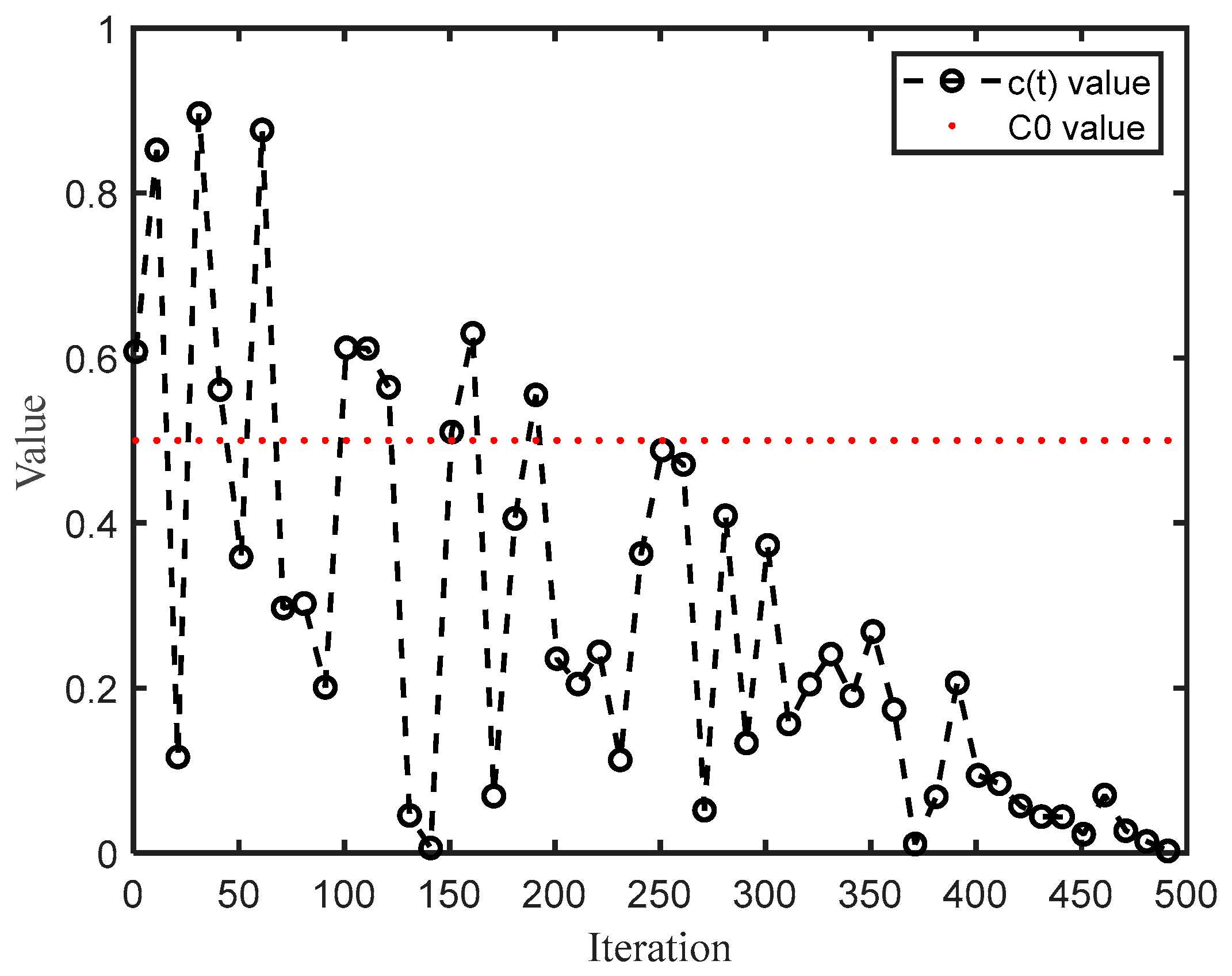
2.4. Time Control Mechanism

In order to capture the type of movement that changes with time, the time control theory needs to be introduced. It controls the passive and active movements of candidate individuals in the colony, and also the movements of candidates going after ocean currents.

In order to adjust different movements of candidate individuals, the time control function C(t) and constant C₀ need to be considered. Figure 1 displays the change trend of the time control function. C(t) is the random value that fluctuates between 0 and 1 from Figure 1, therefore, C₀ is set to 0.5. The candidate individuals follow the ocean current when C(t) > 0.5; otherwise, candidates move within the swarm.

$$C(t)=\left|(1-t/T)\times (2\times \mathrm{rand}(0, 1)-1)\right|$$

(12)

where t and T are the current and maximum iterations, respectively.

Similarly, function 1 − C(t) is also applied to regulate A and B movements of candidates within a swarm. The candidates show passive moving if rand(0, 1) > 1 − C(t), Otherwise, candidates exhibit active moving. Since the value of 1 − C(t) increases from 0 to 1 at the beginning of iteration, then rand(0, 1) > 1 − C(t), at which time, passive moving of candidates takes precedence over active movement of candidates.

2.5. Boundary Conditions

Since the earth is spherical, it returns to the phase when the jellyfish movements exceed the bounded search zone. The process is shown in Equation (13):

$$\left\{\begin{array}{l}{P^{\prime }}_i^d=(P_i^d-U{b}_{}^d)+L{b}_{}^d\hspace{1em}if\hspace{0.17em}{P}_i^d>U{b}^d\\ {P^{\prime }}_i^d=(P_i^d-L{b}^d)+U{b}^d\hspace{1em}if\hspace{0.17em}{P}_i^d<L{b}_{}^d\end{array}\right.$$

(13)

where $P_i^d$ is location of the i-th candidate with the d-th dimension, ${P^{\prime }}_i^d$ is the renewed position after checking boundary constraints, $U{b}^d$ and $L{b}_{}^d$ are the upper and lower limits of the d-th dimension in finding space, respectively.

2.6. Steps of the Jellyfish Search Algorithm

For the JS algorithm, the moving of candidate individuals chasing after the ocean current is called exploration, and the movement of candidate individuals within the swarm is defined as exploitation, and time control parameters control the switch between these two phases. The JS algorithm focuses on exploration to find potential areas at the beginning of iteration; the JS algorithm prefers exploitation to determine the best position in the determined area at the end of the iteration. To summarize the above phases, the exhaustive steps of the JS algorithm are summarized in the following description; meanwhile, the pseudo-code of the JS algorithm is displayed in Algorithm 1:

Step 1. Define the fitness function, set N and T, generate initial positions of N jellyfish individuals in solution search space through logistic maps defined by Equation (1), and let t = 1.

Step 2. Evaluate and compare the objective value of each candidate, and save the optimal location found so far and the corresponding optimal objective value.

Step 3. Compute the time control function C(t) using Equation (12). If C(t) > 0.5, the candidate individual tracts ocean current, and the new location is renewed using Equation (7), otherwise, perform Step 4;

Step 4. Jellyfish move within swarm. If rand(0, 1) > 1−C(t), the candidate individual carries out Type A movement, and the new position is calculated using Equation (8). Otherwise, the candidate carried out Type B movement, and the new position is update using Equation (9).

Step 5. Check the updated individual position whether go beyond boundary condition. If it is out of the search area, Equation (13) is used to return to the opposite boundary.

Step 6. Compare the objective cost of the current location before and after updating. If the fitness value of the updated position is better, replace the current location and corresponding fitness value, and then compare the objective value of the current position with the optimal fitness value. If the objective value of the present location is better, renew the best location found so far and corresponding optimal objective value.

Step 7. If t < T, go back to Step 3, otherwise, perform Step 8.

Step 8. Outlet the best location and corresponding target cost value.

Algorithm 1: JS algorithm

Begin    Step 1: Initialization. Define the objective function, set N and T, initialize population of jellyfish using Logistic map according to Equation (1), and set $t=1$.    Step 2: Objective calculation. Calculate quantity of food at each candidate location, and pick up the optimal location of candidate.    Step 3: While t < T do        for i = 1 to N do           Implement c(t) with Equation (12)          if $C(t)>0.5$ then           Update location with Equation (7)           else           if rand(0, 1) > 1 − C(t) then            Update location with Equation (8)           else            Update location with Equation (9)           end if         end if         Check whether the boundary is out of bounds and and replace the optimal position.         end for        end while    Step 4: Return. Return the global best position and corresponding optimal objective cost fitness value. End

3. Enhanced Jellyfish Search Algorithm

Due to defects of the JS algorithm on some benchmark test functions, such as low calculation precision and easily getting stuck at a local optimal value. in this section, we introduce the following improvements to the JS algorithm, which can enhance the quality of the solution, accelerate convergence, and improve the algorithm’s precision: (i) By adding sine and cosine learning factors, jellyfish learn from the best individual at the same time when moving in Type B motion, which enhances the solution’s quality, and accelerates convergence. (ii) The addition of the local escape operator prevents the JS algorithm from getting stuck at a local optimal value, which improves the exploitation capability of the JS algorithm. (iii) An opposition-based learning and quasi-opposition learning strategy is applied to increase the diversity distribution of candidate populations, and the better individuals in the present solution and the new solution are executed in the next iteration, which enhances the solution’s quality and improves the convergence speed and accuracy of the JS algorithm.

3.1. Sine and Cosine Learning Factors

In the exploration phase of the JS algorithm, when jellyfish move in Type B motion within the jellyfish swarm, the updated position of the jellyfish is only related to another jellyfish randomly selected. In other words, the jellyfish randomly learn from the jellyfish individuals in the current population, which has certain blindness and lacks effective information exchange within the population. This process may lead the algorithm to move away from the orientation of the optimal candidate solution, and at the same time, the convergence speed could be slowed down. In order to ameliorate these deficiencies, the sine and cosine learning factors, i.e., ω₁ and ω₂, are introduced to make jellyfish learn from both random individuals and the best individual in the search range. This strategy improves the quality of the candidate solution during the exploration phase by seeking the best location more quickly and accelerating the convergence speed.

$${\omega }_1=2\cdot \sin [(1-t/T)\cdot \pi /2]$$

(14)

$${\omega }_2=2\cdot \cos [(1-t/T)\cdot \pi /2]$$

(15)

In Type B movement, Equation (16) describes the location update mode of jellyfish:

$$P_i(t+1)={\omega }_1\cdot (P_i(t)+\overrightarrow{step})+{\omega }_2\cdot (P^{\ast }-P_i(t))$$

(16)

where $\overrightarrow{step}$ can see Equations (10) and (11).

The original JS algorithm adopts a random strategy to learn, which makes jellyfish randomly learn from the current individual. Poor fitness values of the learned jellyfish individuals will lead to limited convergence speed. Therefore, the sine and cosine learning factors that are introduced into the JS algorithm make the jellyfish learn from random solutions and follow the optimal solution within the search range, and therefore, quickly improves the quality of the solution and accelerates convergence speed.

3.2. Local Escape Operator

The core of swarm intelligence algorithms is to effectively judge and weigh the exploration and exploitation capability of an algorithm. The added sine and cosine learning factors can increase the JS algorithm’s local exploration capability, but the global exploitation capability is weakened. The local escape operator (LEO) is a local search operator based on a gradient-based optimizer (GBO) [45], which aims to find new areas and to enhance the exploitation capability. Therefore, it is implemented in the phase of jellyfish following the ocean current. Notably, the local search operator can update the position of the candidate $P_i(t+1)$. This helps the algorithm skip any local optimal solutions. Because of this, it can expand the diversity of candidate individuals to search for the global optimal solution. In other words, it makes the algorithm skip the trap of local optimization.

By using multiple solutions such as optimal individual $P^{\ast }$, two randomly candidate solutions $P{1}_i(t)$ and $P{2}_i(t)$, two randomly selected candidate solutions $P_{r1}(t)$ and $P_{r2}(t)$, a new candidate position $P_k(t)$, the LEO gives the alternative solution $P_{LEO}(t)$ of the current solution $P_i(t+1)$, and the generated solution can explore the search space around the optimal solution. See Equations (17) and (18) for a specific mathematical description:

$$\begin{array}{c}\mathrm{if} \mathrm{rand}<0.5\hfill \\ P_{LEO}(t)=P_i(t+1)+f_1(u_1{P}^{\ast }-u_2{P}_k(t))+f_2{\rho }_1(u_3(P{2}_i(t)-P{1}_i(t)))\hfill \\ \hspace{1em}\hspace{1em}\hspace{1em}+u_2(P_{r1}(t)-P_{r2}(t))/2\hfill \\ P_i(t+1)=P_{LEO}(t) \hfill \end{array}$$

(17)

$$\begin{array}{c}\mathrm{else}\hfill \\ P_{LEO}(t)=P^{\ast }+f_1(u_1{P}^{\ast }-u_2{P}_k(t))+f_2{\rho }_1(u_3(P{2}_i(t)-P{1}_i(t)))\hfill \\ \hspace{1em}\hspace{1em}\hspace{1em}+u_2(P_{r1}(t)-P_{r2}(t))/2\hfill \\ P_i(t+1)=P_{LEO}(t)\hfill \\ \mathrm{End}\hfill \end{array}$$

(18)

where f₁ is any number uniformly distributed in [−1, 1], f₂ ~N (0, 1). u₁, u₂, and u₃ are three random numbers with the following mathematical formulae:

$$u_1=L_1\times 2\times R1+(1-L_1)$$

(19)

$$u_2=L_1\times R2+(1-L_1)$$

(20)

$$u_3=L_1\times R3+(1-L_1)$$

(21)

where L₁ is a binary parameter, and L₁ = 0 or 1. If ${\mu }_1$ < 0.5, L₁ = 1, otherwise, L₁ = 0, and ${\mu }_1$ is defined as an arbitrary number between 0 and 1. In addition, ${\rho }_1$ is the adaptive coefficient; R1 = rand(0, 1), R2 = rand(0, 1), and R3 = rand(0, 1) are three random numbers between 0 and 1. Specific definitions are as follows:

$${\rho }_1=2\times \mathrm{rand}(0,1)\times \alpha -\alpha$$

(22)

$$\alpha =|\chi \times \sin (3\pi /2+\sin (\beta \times 3\pi /2))|$$

(23)

$$\chi ={\chi }_{\min }+({\chi }_{\max }-{\chi }_{\min })\times {(1-{(t/T)}^3)}^2$$

(24)

where ${\chi }_{\min }=0.2$, ${\chi }_{\max }=1.2$.

In addition, the following mathematical formulae give two randomly generated solutions $P{1}_i(t)$ and $P{2}_i(t)$:

$$P{1}_i(t)=Lb+R4\times (Ub-Lb)$$

(25)

$$P{2}_i(t)=Lb+R5\times (Ub-Lb)$$

(26)

The meaning of parameter representation is described above. R4 = rand(1, D) and R5 = rand(1, D). The mathematical formula of solution $P_k(t)$ is defined in Equation (27):

$$P_k(t)=L_2\times P_p(t)+(1-L_2)\times P_{rand}$$

(27)

$$P_{rand}=Lb+R6\times (Ub-Lb)$$

(28)

where P_p, p ∈ {1,2, …, N} is an arbitrarily solution, R6 = rand(0, 1) and L₂ is a binary parameter. If ${\mu }_2$ < 0.5, L₂ = 1, otherwise, L₂ = 0. ${\mu }_2=\mathrm{rand}\left(0, 1\right).$

3.3. Learning Strategy

Opposition-based learning (OBL) [46] and quasi-opposition learning (QOL) [47] are both effective methods to increase the diversity of the candidate individuals, the coverage space of solutions, and the performance of the algorithm. After completing the exploration and exploitation phases of the algorithm, with the aim to further increase the solution precision of the JS algorithm, the OBL and QOL strategy is used to update jellyfish individuals according to probability p, and the solution’s quality in the population is enhanced, and then the optimization competence is magnified.

By implementing the OBL and QOL strategy for the i-th candidate individual P_i in the present population, the opposition-based solution and the quasi-opposition solution can be obtained, recorded as ${\tilde{P}}_i=({\tilde{P}}_i^1,{\tilde{P}}_i^2,\cdots ,{\tilde{P}}_i^D)$ and ${\stackrel{⌣}{P}}_i=({\stackrel{⌣}{P}}_i^1,{\stackrel{⌣}{P}}_i^2,\cdots ,{\stackrel{⌣}{P}}_i^D)$. The specific expression of the component is shown in Equations (29) and (30).

$${\tilde{P}}_i^d=L{b}^d+U{b}^d-P_i^d$$

(29)

$${\stackrel{⌣}{P}}_i^d=\mathrm{r}\mathrm{a}\mathrm{n}\mathrm{d}\left(\frac{L{b}^d+U{b}^d}{2},L{b}^d+U{b}^d-P_i^d\right)$$

(30)

where $P_i^d$ is location of the i-th candidate with the d-th dimension, $U{b}_{}^d$ and $L{b}_{}^d$ are the upper and lower limits with the d-th dimension in solution space, respectively.

To sum up, the renewed equation of the i-th candidate jellyfish P_i is defined as the following equation:

$$P_i^{new}=\left\{\begin{array}{l}{\tilde{P}}_i\hspace{1em}if\hspace{0.17em}\mathrm{rand}<p\\ {\stackrel{⌣}{P}}_i\hspace{1em}if\hspace{0.17em}\mathrm{rand}\ge p\end{array}\right.,\hspace{1em}i=1,2,\cdots ,N$$

(31)

where p is selection probability, and p = 0.5.

The algorithm generates N new jellyfish individuals through Equation (31), and then calculates the objective values of the present and new candidates. According to the calculation results, the 2N candidate individuals are sorted, and choose the better N jellyfish individuals to participate in the next iteration process.

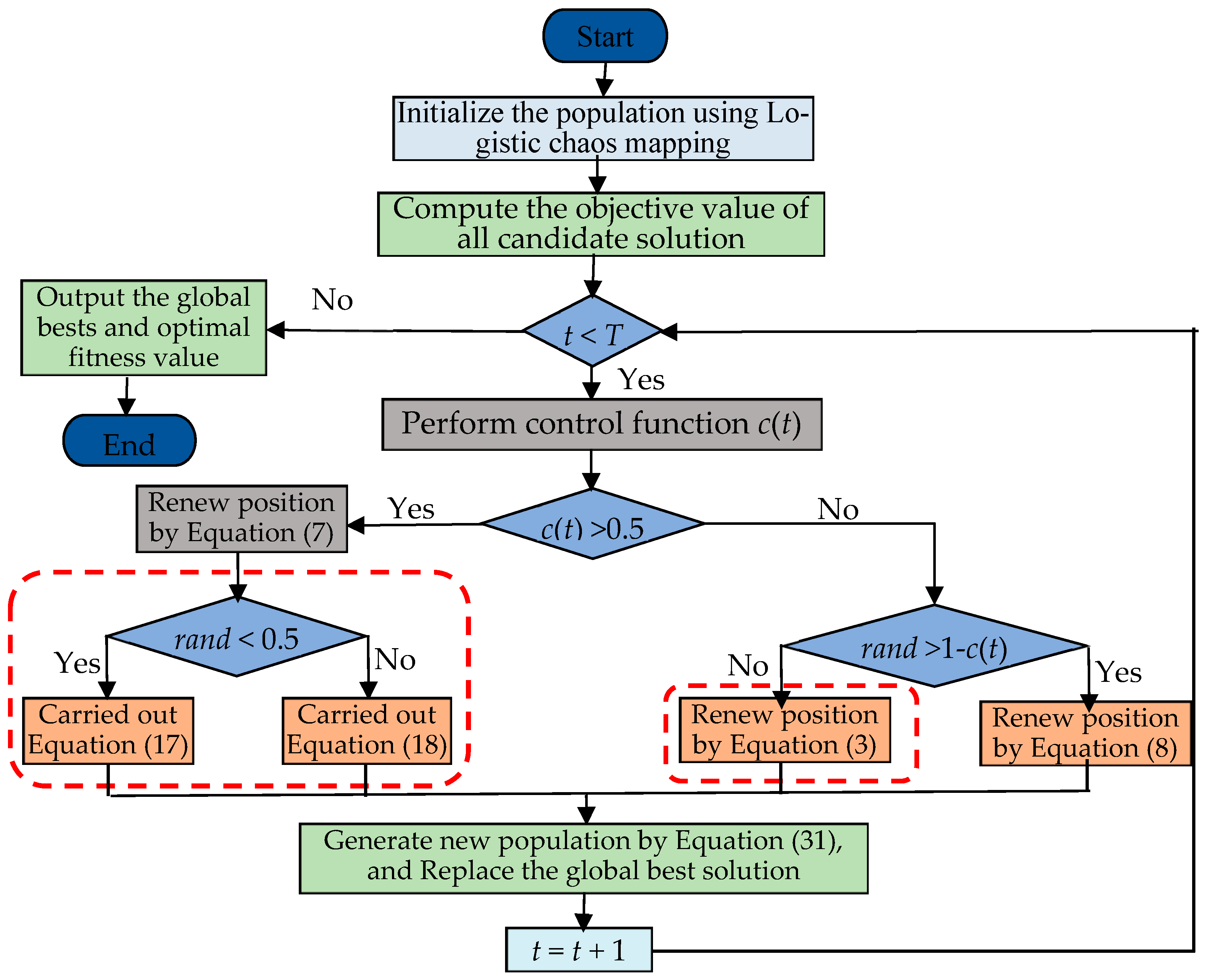
3.4. Steps of Enhanced Jellyfish Search Algorithm

The sine and cosine learning factors strategy improves the local exploration capability and the convergence performance of the algorithm. The local escape operator strategy enhances the global exploitation capability and the capability to skip the trap of local optimization. The OBL and QOL strategy increases the diversity of the candidate individuals, the solution’s quality in population is enhanced, thus magnifying the optimization competence. By combining these three strategies with the JS algorithm, an enhanced jellyfish search algorithm is developed (called the EJS algorithm). The detailed steps of the EJS algorithm are similar to the JS algorithm in Section 2.6. The main difference is that the opposition-based learning and quasi-opposition learning strategy is implemented between Step 4 and Step 5. Figure 2 shows the flow chart of the EJS algorithm to facilitate understanding the entire process. Meanwhile, the pseudo-code of the EJS algorithm is displayed in Algorithm 2.

3.5. Time Complexity of the EJS Algorithm

An algorithm refers to a group of methods used to operate data and to solve program problems. For the same problem, using different algorithms may result in the same result, but the resources and time consumed in the process will vary greatly. So how should we measure the advantages and disadvantages of different algorithms? This article will use time complexity to illustrate. That is, estimate the execution times (execution time) of program instructions.

The time complexity of the EJS algorithm lies on N, D and T. For all iteration period, the EJS algorithm performs the following procedure: candidates follow the ocean current, then the local escape operator is implemented, candidates move in active motion with sine and cosine learning factors or passive motion within a swarm, new individuals are generated through an opposition-based learning and quasi-opposition learning strategy, and better candidate individuals are selected to participate in the iterative process of the next generation. Combined with the above analysis, the time complexity can be calculated. The meaning of T, N, and D can see above content.

$$\begin{array}{c}O(\mathrm{EJS})=O(T(O(\mathrm{candidate}\hspace{0.33em}\mathrm{follow}\hspace{0.33em}\mathrm{ocean}\hspace{0.33em}\mathrm{current}+\mathrm{local}\hspace{0.33em}\mathrm{escaping}\hspace{0.33em}\mathrm{operator})\\ \hspace{1em}\hspace{1em}+O(\mathrm{passive}\hspace{0.33em}\mathrm{motion}+\mathrm{active}\hspace{0.33em}\mathrm{motion})+O(\mathrm{Learning} \mathrm{strategy})))\end{array}$$

(32)

$$O(\mathrm{EJS})=O(T(ND+ND+ND))=O(TND).$$

(33)

Algorithm 2: EJS algorithm

Begin   Step 1: Initialization. Define the fitness function, set N and T, initialize with Logistic map $P_{i+1}=\eta P_i(1-P_i),\hspace{1em}0\le P_0\le 1$ for $i=1,\cdots ,N$, and set $t=1$.   Step 2: Fitness calculation. Calculate quantity of food at each jellyfish position $f_i=f(P_i)$, and pick up the best position $P_{best}$    Step 3: While t < T do         for I = 1 to N do            $C(t)=\left|(1-t/T)\times (2\times rand(0, 1)-1)\right|$          if $C(t)>0.5$ do               $P_i(t+1)=P_i(t)+r2\times (P^{\ast }-\beta \times r2\times \mu )$            //Local escaping operator(LEO)            if rand < 0.5             $\begin{array}{c}{P}_{LEO}(t)=P_i(t+1)+f_1(u_1{P}^{\ast }-u_2{P}_k(t))+f_2{\rho }_1(u_3(P{2}_i(t)-P{1}_i(t)))\\ \hspace{1em}\hspace{1em}\hspace{1em}\hspace{1em}+u_2(P_{r1}(t)-P_{r2}(t))/2\end{array}$            $P_i(t+1)=P_{LEO}(t)$          else             $\begin{array}{c}{P}_{LEO}(t)=P^{\ast }+f_1(u_1{P}^{\ast }-u_2{P}_k(t))+f_2{\rho }_1(u_3(P{2}_i(t)-P{1}_i(t)))\\ \hspace{1em}\hspace{1em}\hspace{1em}\hspace{1em}+u_2(P_{r1}(t)-P_{r2}(t))/2\end{array}$           Pi(t + 1) = PLEO(t)          end         else           if $rand(0,1)>(1-C(t))$ Do   //Type A              $P_i(t+1)=P_i(t)+\gamma \times r3\times (Ub-Lb)$           else   //Type B             //Sine and cosine learning factors                ${\omega }_1=2\cdot \sin [(1-t/T)\cdot \pi /2]$                ${\omega }_2=2\cdot \cos [(1-t/T)\cdot \pi /2]$                $P_i(t+1)={\omega }_1\cdot (P_i(t)+\overrightarrow{\mathrm{step}})+{\omega }_2\cdot (P^{\ast }-P_i(t))$           end if          end if          //Learning strategy             ${\tilde{P}}_i^d=L{b}^d+U{b}^d-P_i^d$             ${\stackrel{⌣}{P}}_i^d=rand\left(\frac{L{b}^d+U{b}^d}{2},L{b}^d+U{b}^d-P_i^d\right)$             $P_i^{new}=\left\{\begin{array}{l}{\tilde{P}}_i\hspace{1em}if\hspace{0.17em}\mathrm{rand}<p\\ {\stackrel{⌣}{P}}_i\hspace{1em}if\hspace{0.17em}\mathrm{rand}\ge p\end{array}\right.,\hspace{1em}i=1,2,\cdots ,N$           Check whether the boundary is out of bounds. If it out of search region, and replace the location;         end for        end while     Step 4: Return. Return the global optimal solution.         End

4. Numerical Experiment and Result Analysis Based on a Benchmark Test Set

To benchmark the performance of the proposed EJS algorithm, 29 benchmark functions from the standard CEC2017 test set and ten benchmark functions from the legal CEC2019 test set are used to execute the experimental sequence. The EJS algorithm is compared with other famous optimization methods. Aiming at unbiased experimental results, all tests are conducted in the same Windows 10 environment; all tests are implemented on Matlab-2018a installed on an Intel(R) Core(TM) i5-8625u CPU @ 1.60 GHz, 1.80 GHz, and 8.00 GB. For all optimization algorithms, set N = 50. In addition, all algorithms are implemented 20 times independently, T = 1000 is the termination condition.

The test sets are both discussed. Due to space limitations, in this article, we only show the CEC2019 test functions in detail. Ten CEC2019 benchmark functions [48] are employed to evaluate the algorithm’s execution. The test functions F4–F10 can be shifted and rotated with the boundary range [−100, 100], while the test functions F1–F3 with different boundary ranges and dimensions cannot be moved and rotated.

Table 1. The details of the CEC2019 test functions.

No	Function Name	Optimal Value	Dim	Search Range
F1	Storn’s Chebyshev Polynomial Fitting Problem	1	9	[−8192, 8192]
F2	Inverse Hilbert Matrix Problem	1	16	[−16,384, 16,384]
F3	Lennard-Jones Minimum Energy Cluster	1	18	[−4, 4]
F4	Rastrigin’s Function	1	10	[−100, 100]
F5	Griewangk’s Function	1	10	[−100, 100]
F6	Weierstrass Function	1	10	[−100, 100]
F7	Modified Schwefel’s Function	1	10	[−100, 100]
F8	Expanded Schaffer’s F6 Function	1	10	[−100, 100]
F9	Happy Cat Function	1	10	[−100, 100]
F10	Ackley Function	1	10	[−100, 100]

gives the details of the CEC2019 test functions.

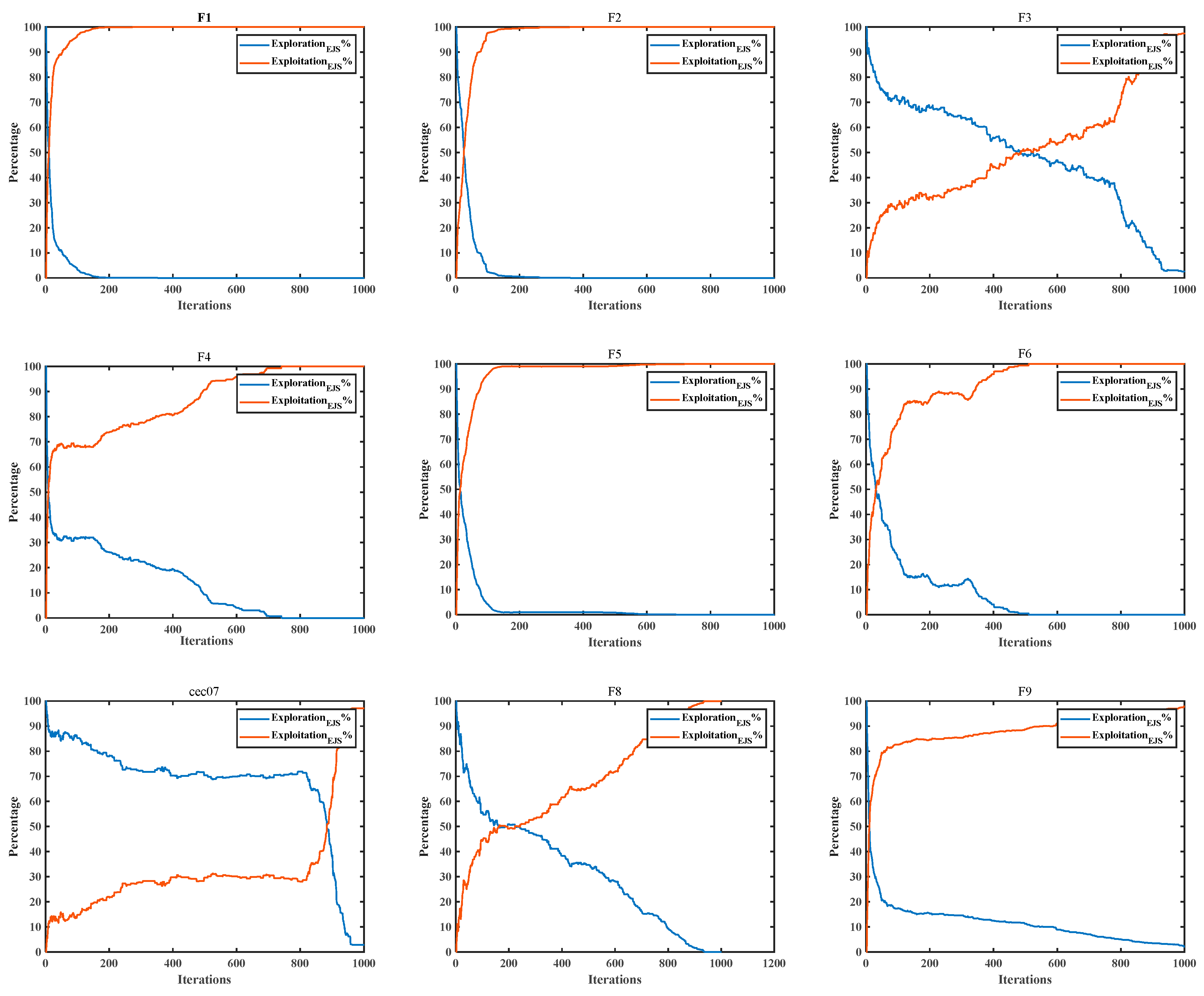
4.1. Performance Indicators

Here, we give six evaluation indicators to accurately analyze the performance of the EJS algorithm [49].

(i) Best value

$$\mathrm{Best}=\min \{bes{t}_1,bes{t}_2,\cdots ,bes{t}_m\}$$

(34)

where $bes{t}_i$ represents the best value of the i-th independent run.

(ii) Worst value

$$\mathrm{Worst}=\max \{bes{t}_1,bes{t}_2,\cdots ,bes{t}_m\}$$

(35)

(iii) Mean value

$$\mathrm{Mean}=\frac{1}{m}{\displaystyle \sum _{i=1}^{m}bes{t}_i}$$

(36)

(iv) Standard deviation

$$\mathrm{Std}=\sqrt{\frac{1}{m-1}{\displaystyle \sum _{i=1}^m{(bes{t}_i-\mathrm{Mean})}^2}}$$

(37)

(v) Rank

The average value of all compared methods are sorted in order, and the corresponding serial number of each algorithm is defined as the rank. If mean values are the same, the standard deviations are further compared. The algorithm with the lowest ranking possesses outstanding performances. Conversely, it indicates that the EJS algorithm is worse than the other compared methods. The average ranking, in this paper, refers to the result obtained by summing the rankings of all test functions of the specified algorithm and dividing it by the total number of test functions.

The median is the number in the middle of a group of data arranged in order, representing a value in a sample population or probability distribution, which can divide the set of values into equal upper and lower parts. Therefore, we also believe that the median can more fairly reflect the ranking of the algorithm. The final ranking is determined by combining the median and the average of the rank. First, the median is used for ranking. When the median is the same, the average rank is considered for the final ranking of all the compared algorithms.

(vi) Wilcoxon rank sum test result

Taking the EJS algorithm as the benchmark, p-values are computed by running other methods for m times, and the statistical results are given at 95% significance level ($\alpha =0.05$). +/=/− are the number of test functions that the EJS algorithm is obviously inferior/equal/superior, respectively, to some famous methods.

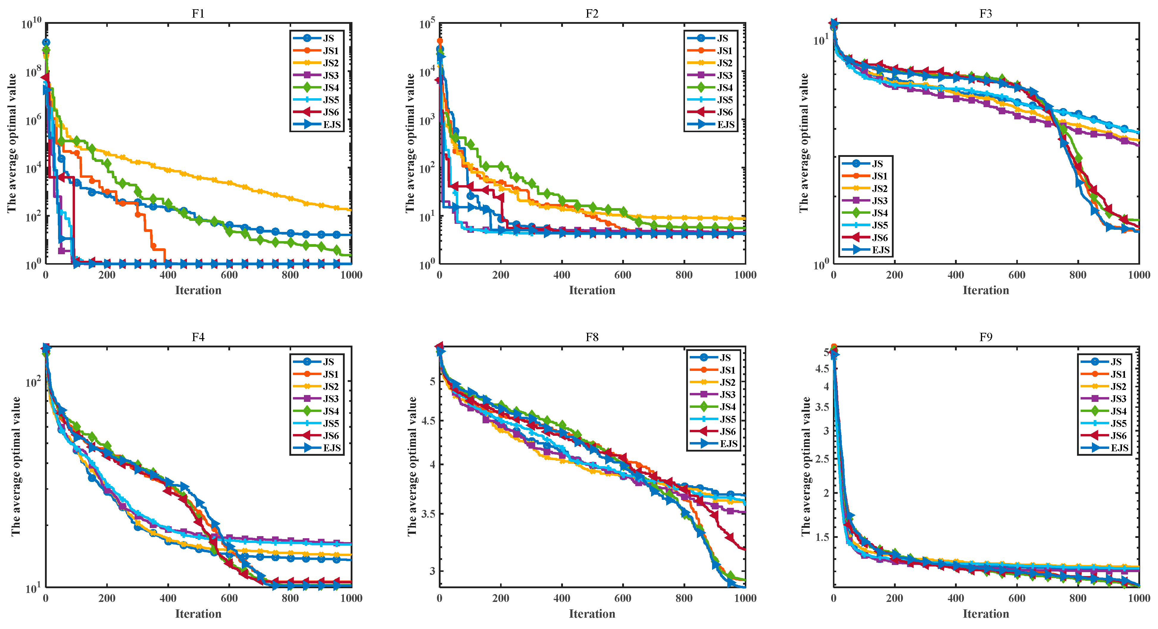
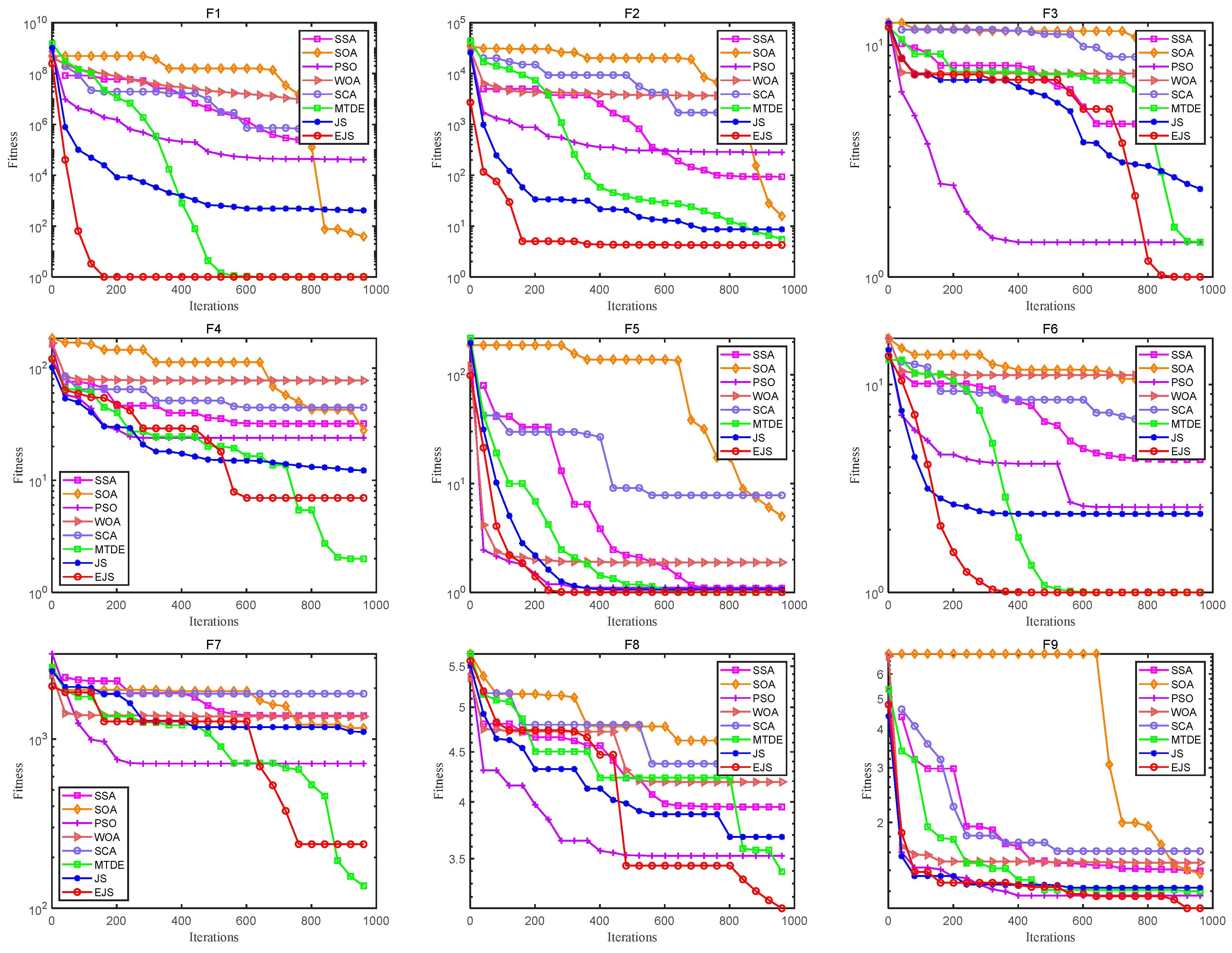
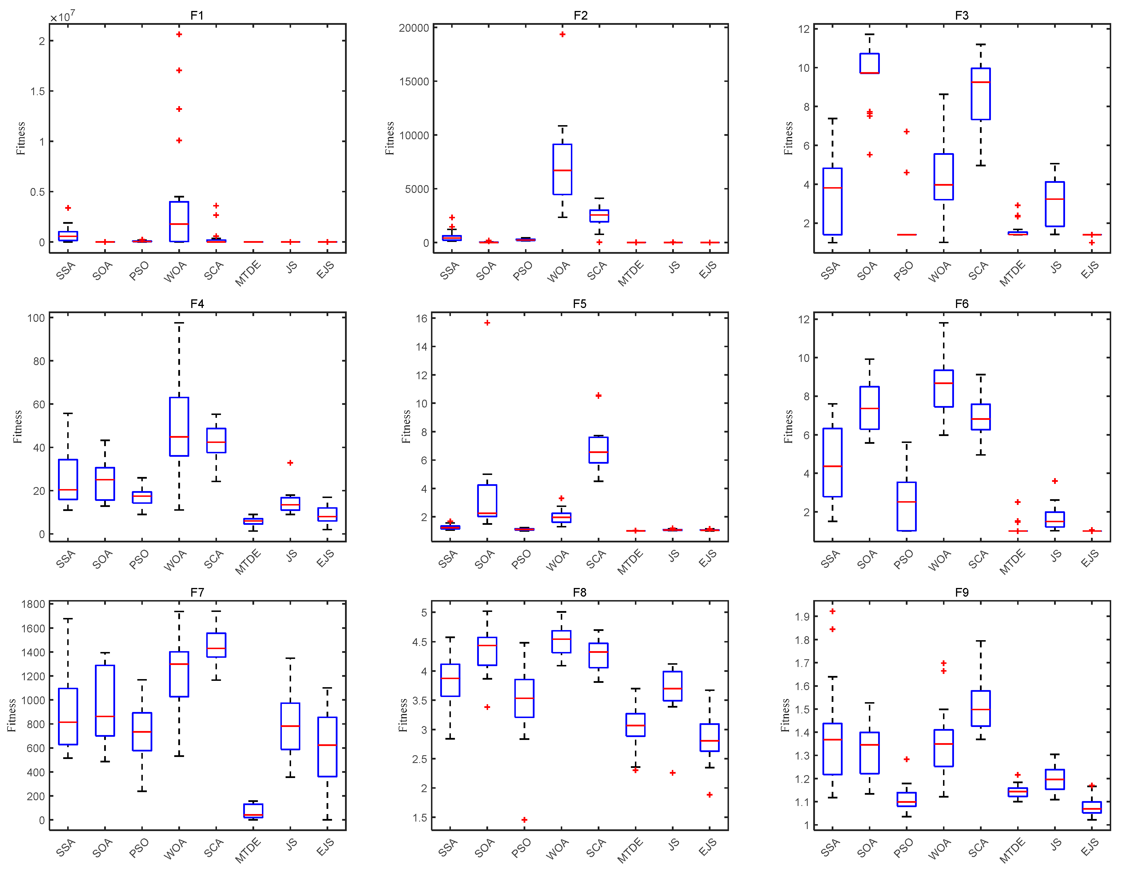
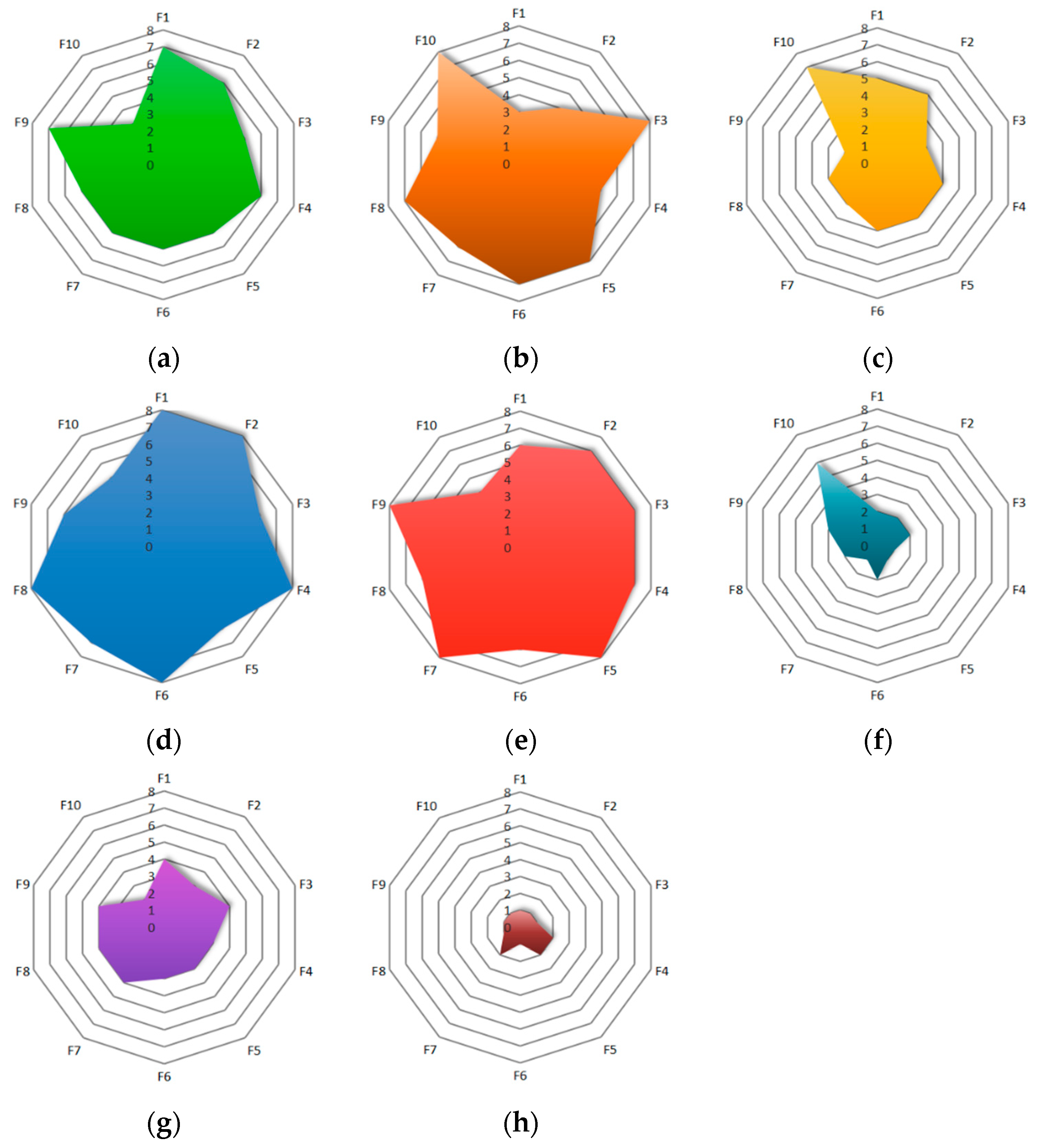
4.2. Comparison between the EJS Algorithm and Other Optimization Algorithms

In order to verify the contribution of each main improvement strategy (the contribution of the individual-based updating strategy) to the performance of the EJS algorithm, the EJS algorithm is compared with its six incomplete algorithms and the JS algorithm. To evaluate the impact of the strategies on convergence speed and accuracy, the incomplete algorithms include the sine and cosine learning factors strategy, the local escape operator strategy, or the learning strategy, corresponding to the JSI, JSII, and JSIII algorithms, respectively, and the select combination strategies corresponding to the JSIV algorithm (the sine and cosine learning factors and the local escape operation), the JSV algorithm (the local escape operator and the learning strategy), and the JSVI algorithm (the learning strategy and the sine and cosine learning factors) algorithm. The selected CEC2019 test set shows references as test function sets. Different function types represent different performances of the algorithms. For details, please refer to Table 1.

The parameter settings are the same as the above. The results including best value, average value, standard deviation, and rank after 20 runs on each test function are summarized in

Table 2. Comparison results of different improvement strategies on the CEC2019 benchmark test functions.

No.	Result	Algorithm
		JS	JSI	JSII	JSIII	JSIV	JSV	JSVI	EJS
F1	Best	1.000000	1.000000	1.000000	1.000000	1.000000	1.000000	1.000000	1.000000
	Worst	107.874719	4.518274	2005.953718	1.000000	34.033461	1.000000	1.000000	1.000000
	Mean	25.353117	1.714772	730.661957	1.000000	7.867176	1.000000	1.000000	1.000000
	Std	4.6579 × 101	1.5674 × 100	8.7582 × 102	8.1288 × 10−8	1.4638 × 100	4.0521 × 10−9	2.2238 × 10−11	4.0951 × 10−13
	Rank	7	5	8	4	6	3	2	1
F2	Best	4.246899	4.198636	4.266541	4.186653	3.908319	4.222719	4.096543	4.225043
	Worst	26.384846	5.010327	8.670419	4.548559	11.681408	4.358863	4.269076	4.274394
	Mean	9.976218	4.455787	5.476164	4.317989	6.827503	4.274081	4.246312	4.265880
	Std	9.3415 × 100	3.2849 × 10−1	1.8428 × 100	1.2939 × 10−1	3.1694 × 100	4.8525 × 10−2	1.4885 × 10−2	5.7127 × 10−3
	Rank	8	5	6	4	7	3	1	2
F3	Best	1.409205	1.409135	1.423200	1.419679	1.000000	2.133738	1.409135	1.000001
	Worst	5.9568	1.4140	5.1663	5.1481	4.6081	5.6611	2.2787	1.4497
	Mean	3.829589	1.409379	3.541565	3.371766	1.567780	3.861664	1.462579	1.390706
	Std	1.4241 × 100	1.0867 × 10−3	1.0588 × 100	1.1612 × 100	7.2708 × 10−1	1.0251 × 100	1.9616 × 10−1	9.2406 × 10−2
	Rank	7	2	6	5	4	8	3	1
F4	Best	5.974795	4.979836	7.964708	8.959667	5.974795	7.965020	3.984877	1.994959
	Worst	19.904187	20.899141	22.579489	24.878957	21.894100	27.720452	19.904187	22.889059
	Mean	13.571367	10.651094	14.364349	16.351025	10.253112	16.154598	10.601347	10.203363
	Std	4.2744 × 100	4.5320 × 100	4.4084 × 100	4.4952 × 100	4.1478 × 100	4.4344 × 100	4.5683 × 100	5.2338 × 100
	Rank	5	4	6	8	2	7	3	1
F5	Best	1.000391	1.009865	1.019678	1.003905	1.007396	1.009858	1.007396	1.000001
	Worst	1.164923	1.256066	1.127889	1.201756	1.130397	1.129320	1.132895	1.120643
	Mean	1.062980	1.067922	1.065941	1.058357	1.064226	1.059325	1.059564	1.002496
	Std	4.3754 × 10−2	5.8209 × 10−2	2.8223 × 10−2	5.5578 × 10−2	3.7415 × 10−2	3.0438 × 10−2	3.2596 × 10−2	3.4416 × 10−2
	Rank	5	8	7	2	6	3	4	1
F6	Best	1.010457	1.000000	1.008890	1.033805	1.000000	1.030205	1.000000	1.000000
	Worst	3.125804	2.576493	3.071817	4.085525	2.576352	4.234450	1.008229	1.002320
	Mean	1.799196	1.140360	1.629071	1.900689	1.154138	2.045131	1.000851	1.000247
	Std	6.3932 × 10−1	3.9503 × 10−1	6.3335 × 10−1	1.0009 × 100	4.7352 × 10−1	8.5399 × 10−1	2.3623 × 10−3	7.0205 × 10−4
	Rank	6	3	5	7	4	8	2	1
F7	Best	263.387643	119.875516	475.665511	24.567441	432.363813	165.724634	134.682820	123.243229
	Worst	1.1952 × 103	1.2673 × 103	1.3974 × 103	1.1286 × 103	1.1644 × 103	1.3881 × 103	1.2171 × 103	1.2086 × 103
	Mean	745.119061	615.341713	889.860067	711.903040	757.697432	874.636013	577.351162	702.483287
	Std	2.3229 × 102	3.0147 × 102	2.4962 × 102	2.8263 × 102	2.0552 × 102	3.2378 × 102	2.5476 × 102	2.8796 × 102
	Rank	5	2	8	4	6	7	1	3
F8	Best	3.110874	2.197454	2.839690	2.043254	1.758220	3.274288	2.566743	1.717564
	Worst	4.101536	3.813682	4.261395	4.032497	3.647034	3.938084	4.097482	3.809025
	Mean	3.677661	2.928565	3.614662	3.518221	2.927741	3.586926	3.179098	2.871277
	Std	2.4798 × 10−1	4.3209 × 10−1	4.0743 × 10−1	4.2721 × 10−1	5.0958 × 10−1	1.7740 × 10−1	4.2090 × 10−1	4.8730 × 10−1
	Rank	8	3	7	5	2	6	4	1
F9	Best	1.108133	1.047001	1.170710	1.081691	1.040930	1.133197	1.035531	1.040001
	Worst	1.385159	1.157980	1.294128	1.379456	1.144856	1.376869	1.149305	1.128768
	Mean	1.209967	1.096928	1.235022	1.202045	1.080990	1.223293	1.090168	1.080195
	Std	6.9719 × 10−2	2.7865 × 10−2	3.9300 × 10−2	7.4747 × 10−2	2.8149 × 10−2	6.2415 × 10−2	3.2839 × 10−2	2.8916 × 10−2
	Rank	6	4	8	5	2	7	3	1
F10	Best	11.6185	7.491409	1.000001	1.000000	1.000000	3.013315	3.013315	1.000000
	Worst	21.5071	21.511923	21.452565	21.496805	21.501699	21.534074	21.539023	21.500175
	Mean	20.0395	20.701859	16.406949	15.824920	18.436521	18.611377	19.590365	17.416985
	Std	1.05 × 101	3.1102 × 100	8.0406 × 100	8.3796 × 100	7.1870 × 100	6.0449 × 100	5.5736 × 100	8.1379 × 100
	Rank	7	8	2	1	4	5	6	3
Mean Rank		6.5	4.2	6.3	4.5	4.3	5.7	2.9	1.5
Median Rank		6.5	4	6.5	4.5	4	6.5	3	1
Result		8	3	7	5	4	6	2	1

. Numbers marked with black font represent the best results on each evaluation index.

From Table 2, all the evaluating indicators of the EJS algorithm and most of the incomplete algorithms are better than the JS algorithm, except for function test F10; therefore, this is adequate to show that the three strategies added in this paper improve the original algorithm to a certain extent. The JS algorithm can obtain the optimal solution except for on test functions F2, F4, and F8. On the individual functions, the improvement of the three strategies is not as good as the improvement of the original algorithm using a single strategy. For example, for test function F2, the effect of the JSVI algorithm is better than that of the EJS algorithm, that is, the local escape operator may cause the accuracy of the algorithm to be reduced on test function F2. The effect of the EJS algorithm is inferior to the JSI and JSIII algorithms on test function F7, that is, the sine and cosine learning factors strategy and the learning strategy may cause the accuracy of the algorithm to be reduced on test function F7. The effects of the JSII and JSIII algorithms are superior to the EJS algorithm on test function F10, that is, the local escape operator strategy and the learning strategy may cause the accuracy of the algorithm to be reduced on function F10, but the difference is not large; the best values are obtained using JSIV and JSIII, however, they all fluctuate slightly near the optimal solution. From the overall ranking, the ranking order of the eight algorithms is EJS > JSVI > JSI > JSIV > JSIII > JSV > JSII > JS. These results show that the EJS algorithm is able to avoid local optimal solutions and find better solutions by using the local escape operator, which is consistent with the analysis in Section 3.2. The performance of the EJS algorithm in solving accuracy and stability is comparable to the JS algorithm on all functions, and therefore, the theoretical optimal value has been found.

Due to article space constraints, in this paper, we only present the convergence curves of some test sets in Figure 3. It can be seen from the figure that the convergence speed and accuracy of the JSI algorithm is improved, the convergence speed and accuracy of the JSII, JSIII, JSV, and JSVI algorithms are improved, and the JSIII algorithm is relatively obvious, that is to say, the learning strategy can significantly improve the calculation accuracy, accelerate convergence speed, and avoid falling into local optimization.

The EJS algorithm is compared with some other recognized optimization methods (such methods include JS [23], HHO [19], GBO [45], WOA [14], AOA [11], SCA [50], BMO [20], SSA [51], SOA [21], PSO [12], and MTDE [52]) to further prove the performance of the EJS algorithm.

Table 3. Related parameters of other recognized algorithms.

Algorithm	Parameter	Value
JS	C0	0.5
EJS	C0	0.5
	Selection probability p	0.5
HHO	Initial energy E0	[−1, 1]
GBO	Constant parameters	βmin = 0.2, βmax = 1/2
	Probability parameter pr	0.5
WOA	a, b	Decreasing from 2 to 0 with linearly 1
AOA	C	C1 = 2, C2 = 6, C3 = 1, C4 = 2
SCA	a	2
BMO	pl	7
SSA	Initial speed v0	0
SOA	Control Parameter A	Decreasing from 2 to 0 with linearly
	The value of fc	0
PSO	Cognitive coefficient	2
	Social coefficient	2
	Inertia constant	decreases from 0.8 to 0.2 linearly
MTDE	Constant parameters	WinIter = 20, H = 5, initial = 0.001, final = 2, Mu = log(D), μf = 0.5, σ = 0.2

provides related parameter settings of these recognized methods.

Each benchmark function is carried out 20 times on the CEC2019 test set.

Table 4. Results of the EJS algorithm and other optimization algorithms on the CEC2019 test set.

No.	Result	Algorithm
		SSA	SOA	PSO	WOA	SCA	MTDE	JS	EJS
F1	Best	2.03 × 103	1	7.46 × 103	1.57 × 102	1	1	1	1
	Worst	3.39 × 106	2.38 × 102	2.30 × 105	2.06 × 107	3.60 × 106	1.0001	9.62 × 103	1
	Mean	7.55 × 105	2.28 × 101	7.18 × 104	4.22 × 106	3.87 × 105	1	5.61 × 102	1
	Std	6.94 × 1011	3.33 × 103	3.61 × 109	3.72 × 1013	9.30 × 1011	4.33 × 10−1	4.57 × 106	1.56 × 10−24
	MeanFEs	50,050	50,000	50,000	50,000	50,000	50,050	50,050	4,269,450
	Rank	7	3	5	8	6	2	4	1
F2	Best	1.37 × 102	4.2578	1.51 × 102	2.36 × 103	2.81 × 101	3.6598	4.0952	4.1721
	Worst	2.33 × 103	2.02 × 102	4.40 × 102	1.94 × 104	4.13 × 103	1.63 × 101	4.05 × 101	4.2865
	Mean	5.86 × 102	3.39 × 101	2.61 × 102	7.21 × 103	2.42 × 103	6.7871	8.3173	4.2474
	Std	2.95 × 105	2.99 × 103	7.68 × 103	1.52 × 107	1.09 × 106	8.5241	6.44 × 101	8.34 × 10−4
	MeanFEs	50,050	50,000	50,000	50,000	50,000	50,050	50050	4,278,650
	Rank	6	4	5	8	7	2	3	1
F3	Best	1	5.5227	1.4091	1.0114	4.9662	1.4092	1.4190	1
	Worst	7.3871	11.7128	6.7120	8.6335	11.1873	2.9206	5.0663	1.4101
	Mean	3.5624	9.6919	2.0993	4.3972	8.7119	1.6112	3.0739	1.3683
	Std	3.4887	2.3448	2.9966	5.0363	3.021	1.80 × 10−1	1.3527	1.59 × 10−2
	MeanFEs	50,050	50,000	50,000	50,000	50,000	50,050	50,050	4,288,670
	Rank	5	8	3	6	7	2	4	1
F4	Best	10.9496	12.8433	8.9597	11.0267	24.2144	1.3311	8.9597	1.9950
	Worst	55.7222	43.2380	25.8739	97.5722	55.3016	8.9603	32.8386	16.9193
	Mean	25.2778	24.5804	16.6427	50.0062	41.7837	5.7551	14.1974	9.1587
	Std	153.3892	88.2880	22.2697	508.0421	84.6501	4.6816	29.5700	16.9436
	MeanFEs	50,050	50,000	50,000	50,000	50,000	50,050	50,050	4,287,350
	Rank	6	5	4	8	7	1	3	2
F5	Best	1.0566	1.4885	1	1.2966	4.5055	1	1.0172	1.0099
	Worst	1.6835	15.6787	1.2437	3.3065	10.5726	1.0319	1.1846	1.1454
	Mean	1.2653	3.4743	1.1169	2.0409	6.8461	1.0059	1.0728	1.0625
	Std	2.98 × 10−2	9.4315	4.71 × 10−3	2.52 × 10−1	2.3672	9.52 × 10−5	1.81 × 10−3	1.55 × 10−3
	MeanFEs	50,050	50,000	50,000	50,000	50,000	50,050	50,050	4,282,650
	Rank	5	7	4	6	8	1	3	2
F6	Best	1.5031	5.5717	1	5.9743	4.9522	1	1.015	1
	Worst	7.6048	9.9222	5.6087	11.8140	9.1251	2.500	3.5932	1.0596
	Mean	4.4052	7.4945	2.4119	8.5441	6.9821	1.1239	1.674	1.0034
	Std	3.9027	1.8243	1.9215	2.0366	1.1457	1.28 × 10−1	4.30 × 10−1	1.78 × 10−4
	MeanFEs	50,050	50,000	50,000	50,000	50,000	50,050	50,050	4,280,150
	Rank	5	7	4	8	6	2	3	1
F7	Best	5.16 × 102	4.86 × 102	2.38 × 102	5.33 × 102	1.17 × 103	1.2575	3.57 × 102	1.3747
	Worst	1.67 × 103	1.39 × 103	1.17 × 103	1.74 × 103	1.74 × 103	1.57 × 102	1.35 × 103	1.10 × 103
	Mean	8.93 × 102	9.36 × 102	7.26 × 102	1.23 × 103	1.45 × 103	6.77 × 101	7.93 × 102	5.81 × 102
	Std	1.02 × 105	1.01 × 105	7.03 × 104	9.80 × 104	2.14 × 104	3.04 × 103	7.60 × 104	1.20 × 105
	MeanFEs	50,050	50,000	50,000	50,000	50,000	50,050	50,050	4,271,650
	Rank	5	6	3	7	8	1	4	2
F8	Best	2.8406	3.3827	1.4577	4.0885	3.8107	2.3048	2.2607	1.8870
	Worst	4.5761	5.0174	4.4825	5.0042	4.6990	3.6979	4.1202	3.6695
	Mean	3.8634	4.3280	3.4510	4.5452	4.2684	3.0618	3.6681	2.8739
	Std	2.10 × 10−1	1.29 × 10−1	3.96 × 10−1	8.09 × 10−2	7.10 × 10−2	1.46 × 10−1	1.69 × 10−1	1.96 × 10−1
	MeanFEs	50,050	50,000	50,000	50,000	50,000	50,050	50,050	4,282,450
	Rank	5	7	3	8	6	2	4	1
F9	Best	1.1179	1.1342	1.0353	1.1215	1.3690	1.1001	1.1084	1.0222
	Worst	1.9214	1.5262	1.2829	1.6979	1.7938	1.2156	1.3049	1.1698
	Mean	1.3812	1.3216	1.1108	1.3552	1.5182	1.1440	1.1981	1.0788
	Std	4.82 × 10−2	1.26 × 10−2	3.11 × 10−3	2.22 × 10−2	1.44 × 10−2	8.23 × 10−4	3.68 × 10−3	1.57 × 10−3
	MeanFEs	50,050	50,000	50,000	50,000	50,000	50,050	50,050	4,289,150
	Rank	7	5	2	6	8	3	4	1
F10	Best	20.9965	21.1771	21.0431	21.0073	15.0350	21.0899	11.6185	2.1551
	Worst	21.1029	21.5108	21.4662	21.3630	21.5155	21.2469	21.5071	21.5214
	Mean	21.0130	21.3651	21.2159	21.1252	21.0376	21.1722	20.0395	18.6298
	Std	1.10 × 10−3	8.41 × 10−3	1.04 × 10−2	1.04 × 10−2	2.0042	2.42 × 10−3	1.05 × 101	4.58 × 101
	MeanFEs	50,050	50,000	50,000	50,000	50,000	50,050	50,050	4,287,350
	Rank	3	8	7	5	4	6	2	1
Mean Rank		5.4	6.0	4.0	7.0	6.7	2.2	3.4	1.3
Medial Rank		5	6.5	4	7.5	7	2	3.5	1
Result		5	6	4	8	7	2	3	1

summarizes the evaluation index results for the EJS algorithm and other methods, including the best, worst, mean, standard devation, and rank; the optimal value is highlighted in bold among all the compared algorithms. Based on the data in Table 4, the optimization capability of the EJS algorithm is significantly better than the original JS algorithm on all test function, which may be due to the introduction of the sine and cosine learning factors, local escape operator, and learning strategies that have significantly accelerated the calculation speed and enhanced the calculation precision.

Among eight optimization algorithms, the EJS algorithm has more significant advantages in solving the CEC2019 test set. From the rank of algorithms, except for test functions F4, F5, and F7, the EJS algorithm ranks first on the remaining test functions. Especially on test function F1, the EJS algorithm is significantly superior to the other algorithms; the theoretical optimal value is obtained, and has a very small standard deviation. However, the other optimization algorithms, including the original JS algorithm, are far from the theoretical optimal value. The MTDE algorithm is in line with the theoretical optimal value, but its stability is not as good as the EJS algorithm. In conclusion, the EJS algorithm can significantly accelerate convergence speed, and can improve the calculation precision.

The final ranking of the last row in Table 4 shows a research phenomenon: The performance ranking of the compared algorithms is WOA < SCA < SOA < SSA < PSO < JS < MTDE < EJS, which fully shows that the three strategies introduced in the EJS algorithm significantly accelerate convergence speed and improve the calculation precision of the JS algorithm. This verifys the effectiveness and applicability of the EJS algorithm, which are further confirmed on the CEC2019 test set.

It can be seen from Table 4 that the evaluation times of the fitness value of the original algorithms (JS, SSA, PSO, WOA, SCA, and MTDE) are the same, but the meanFE values of the test functions are different for the EJS algorithm. The average FEs value of 20 times is given in Table 4. It can also be seen that the EJS algorithm has improved the accuracy and convergence speed, but its required space storage and calculation time have increased, which further verifies the complexity highlighted in Section 3.5.

Under a 95% significance level ($\alpha =0.05$) with the EJS algorithm as the benchmark, the Wilcoxon rank sum test values and statistical data of the other compared methods, implemented 20 times on the CEC2019 test set, are listed in

Table 5. p-value results on the CEC2019 test set with the EJS algorithm as the benchmark.

Function	Algorithm
	SSA	SOA	PSO	WOA	SCA	MTDE	JS
F1	6.791 × 10−8	6.791 × 10−8	6.791 × 10−8	6.791 × 10−8	6.791 × 10−8	6.791 × 10−8	6.791 × 10−8
F2	6.791 × 10−8	2.56 × 10−7	6.791 × 10−8	6.791 × 10−8	6.791 × 10−8	1.60 × 10−5	1.20 × 10−6
F3	1.35 × 10−3	6.791 × 10−8	4.20 × 10−3	9.13 × 10−7	6.791 × 10−8	1.66 × 10−7	6.791 × 10−8
F4	1.37 × 10−6	7.93 × 10−7	4.15 × 10−5	1.65 × 10−7	6.78 × 10−8	2.56 × 10−2	2.04 × 10−3
F5	2.06 × 10−6	6.791 × 10−8	6.04 × 10−3	6.791 × 10−8	6.791 × 10−8	1.92 × 10−7	4.90 × 10−1
F6	4.001 × 10−8	4.001 × 10−8	1.14 × 10−6	4.001 × 10−8	4.001 × 10−8	2.15 × 10−2	5.45 × 10−8
F7	1.33 × 10−2	3.64 × 10−3	1.99 × 10−1	5.17 × 10−6	6.791 × 10−8	5.90 × 10−5	8.10 × 10−2
F8	2.06 × 10−6	1.06 × 10−7	5.631 × 10−4	6.791 × 10−8	6.791 × 10−8	1.48 × 10−1	1.25 × 10−5
F9	1.92 × 10−7	1.06 × 10−7	4.68 × 10−2	9.17 × 10−8	6.791 × 10−8	2.04 × 10−5	9.13 × 10−7
F10	1.61 × 10−4	9.68 × 10−1	8.35 × 10−4	3.05 × 10−4	3.512 × 10−1	1.614 × 10−4	3.94 × 10−1
+/=/−	0/0/10	0/1/9	0/1/9	0/0/10	0/1/9	3/1/6	0/3/7

. Wilcoxon rank sum test values that exceed 0.05 are highlighted in bold, which means that the EJS algorithm and the compared algorithms have competitiveness, and they are roughly the same. Combined with the ranking in Table 4, the statistical results of the last line in Table 5 are 0/0/10, 0/1/9, 0/1/9, 0/0/10, 0/1/9, 3/1/6, and 0/3/7. The numbers of functions that the EJS algorithm is significantly better than the SSA, WOA, SOA, PSO, SCA, MTDE, and JS algorithms are 10, 10, 9, 9, 9, 6, and 7, respectively. Therefore, for the CEC2019 test set, the computational accuracy of the EJS algorithm is significantly improved on seven test functions as compared with the original JS algorithm, and the EJS algorithm also has strong competitiveness as compared with the other compared algorithms.

The convergence curves of the EJS algorithm on the test functions are shown in Figure 4 in order to better evaluate the EJS algorithm. As indicated in the figure, for the CEC2019 test set, the EJS algorithm has obviously improved convergence characteristics as compared with the JS algorithm. On test functions F1, F2, F6, and F9, the EJS algorithm accelerates convergence speed, and also increases calculation precision. On test functions F3, F7, and F8, although the convergence speed of the EJS algorithm is not better than that of the PSO algorithm, its convergence does not stop at the late iteration, skipping the trap of local optimization, and its calculation precision is obviously better than the PSO algorithm. The solution’s precision of the EJS algorithm is obviously better than the MTDE algorithm on test functions F4 and F7, but the calculation rate of the MTDE algorithm is slightly slower on each test function, and the EJS algorithm performs well on other test functions. On balance, the convergence curves show that the proposed EJS algorithm has remarkably improved convergence characteristics as compared with the JS algorithm and the additional compared methods, it accelerates convergence speed and correspondingly improves the calculation precision.

The box plots can help researchers to understand and to explain the distribution characteristics obtained with all the algorithms’ solutions. The box plots of the EJS algorithm and the other eight optimization methods on the CEC2019 test set are shown in Figure 5. They show that the median of the EJS algorithm running 20 times is small, except for function tests F4 and F7, which verifies the superiority and effectiveness of the EJS algorithm. At the same time, the rectangular area of the EJS algorithm is clearly narrower than the other methods on function tests F1~F3, F5, and F6, which illustrates that the EJS algorithm has strong stability. The approximate solution can be obtained on almost all time runs. In addition, the height between the upper and the lower quartile is low, indicating that the solution of the EJS algorithm has high consistency. In terms of the EJS algorithm outliers, function test F3, F8, and F9 have fewer outliers, which shows that the EJS algorithm avoids the existence of contingency, and the solution obtained in each iteration is slightly affected by the random strategy. In general, the EJS algorithm is more stable and more accurate than the other compared algorithms.

The radar graphs drawn according to the ranking of all the compared algorithms on the CEC2019 test set are displayed in Figure 6. The radar graphs illustrate that the EJS algorithm has the smallest shadow area, and the algorithm has the smallest comprehensive ranking on the test function. Therefore, the stability of the EJS algorithm is improved. In general, the performance of the EJS algorithm is more valuable than the other compared algorithms on the CEC2019 benchmark.

The difference between individual dimensions can infer whether the group is divergent or clustered in the centralized space. On the one hand, when the algorithm diverges, the difference of the dimension of the group body increases, that is, the group individuals disperse in the search environment. This is called exploration or diversification in metaheuristic research. On the other hand, when the population converges, the difference is minimized and the population individuals gather in a concentrated region. This is called development or reinforcement. In the iterative process, different metaheuristic algorithms adopt different strategies to explore and develop within the group. The concept of exploration and development is ubiquitous in any metaheuristic algorithm. Through exploration, an algorithm can access the invisible community in the search environment to maximize the efficiency of finding the global optimal location. On the contrary, development is the use of neighbors that allow individuals to successfully converge to a potential global optimal solution. The balance between these two capabilities is a trade-off. Neither of these two algorithms can produce effective results. Therefore, maintaining the correct collaboration between the exploration and development modes among algorithms is a necessary condition to ensure the optimization ability. In this paper, we use the dimensional diversity measure proposed by Hussain et al. in [53] for reference to calculate the corresponding exploration and production ratio. Figure 7 shows the exploration and development analysis diagrams of some CEC2019 test functions.

From the figure, we can see that the EJS algorithm starts from the exploration on all test functions, and then gradually transitions to the development stage, i.e., the EJS algorithm with average exploration above 80% and exploitation below 20% on all functions. On test functions F1,F2, F5, and F9, the EJS algorithm can still maintain an effective investigation rate in the middle and early stages of the iteration. On test function F7, the EJS algorithm quickly turns to an effective exploration rate in the middle stage, and ends the iteration with an effective exploitation situation. This discovery process shows that the more effective exploration speed of the EJS algorithm in the early stage ensures reasonable full-range discovery capability to prevent falling into the current local solution. In contrast, the more effective development speed in the later stage ensures that the mining can be carried out with higher accuracy after high exploration.

5. Engineering Application

As more and better intelligent algorithms are proposed, we need to verify their universality and applicability in solving practical engineering problems. All engineering problems can ultimately be summed up as optimization problems. We need to select various design and optimization engineering problems to verify the effectiveness and wide applicability of the algorithm in this paper. Therefore, six different engineering examples are selected, which represent different types of optimization problems, including constrained, unconstrained, discrete variable, continuous variable, mixed variable, implicit constraint, strong constraint, and weak constraint.

The EJS algorithm and some previous methods with the ability to solve practical problems are verified in this section. Here, six engineering cases consist of tension/compression spring design, pressure vessel design, gear set design, cantilever beam design, 3-bar truss design, and 25 bar truss tower design to illustrate the EJS algorithm’s applicability and effectiveness in solving practical engineering problems. The calculation indexes can reflect the practical application effect of the EJS algorithm. In addition to the gear train design, the other five engineering optimization problems are nonlinear constrained optimization problems, which have strong nonlinear objective function and constraint conditions. In this paper, the penalty function is selected to deal with the constraints; it is a technique to deal with nonlinear constraints effectively. Its basic principle is to impose a penalty term on the original, goal expression equation, and then transform the constrained into an unconstrained optimization problem, which is easy to solve with intelligent algorithms including the EJS algorithm. In all experiments, the running environment is the same as in Section 4.1, and set D = 50, T = 1000.

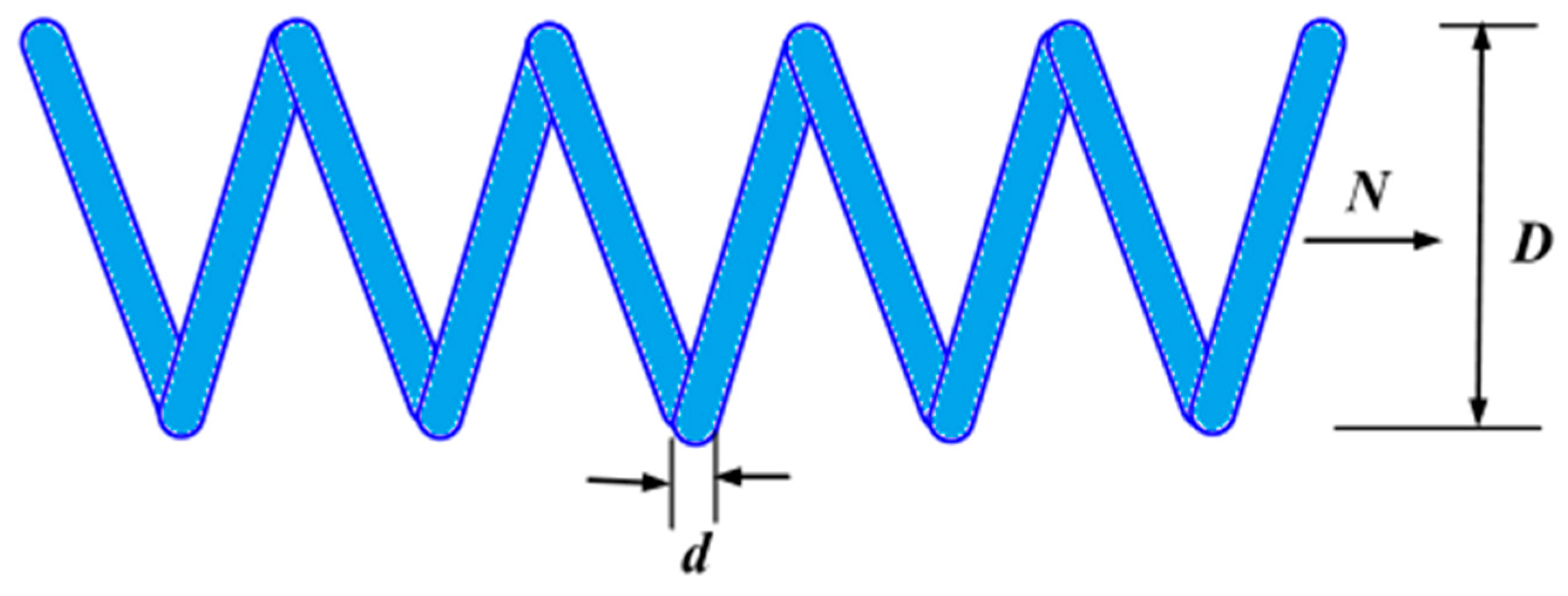
5.1. Tension/Compression Spring Design Problem

The tension/compression spring design problem is a nonlinear constrained optimization issue. The objective is to determine the minimum weight, and the variables that can participate in the optimization are mean coil diameter (D), wire diameter (d), and number of effective coils (N). Figure 8 gives the sketch map of this case. Consider $Z=[z_1,z_2,z_3]=[d,D,N]$, the mathematical expressions of the spring design problem are shown in Equation (38). z₁∈[0.05, 2], z₂∈[0.25, 1.3], and z₃∈[2, 15] are the search areas of this issue.

$$\mathrm{Minimize} \hspace{1em}\hspace{1em}\hspace{1em}\hspace{1em}W(Z)=(z_3+2)z_2{z}_1^2$$

(38)

$$\begin{array}{c}\hspace{1em}\hspace{1em}\hspace{1em}\hspace{1em}\hspace{1em}\hspace{1em} \hspace{1em}\hspace{1em}\hspace{1em}\hspace{1em}\hspace{1em}\hspace{1em}\hspace{1em}\mathrm{Subject} \mathrm{to} \hspace{1em} h_1(Z)=\frac{4z_2^2-z_1{z}_2}{12566(z_2{z}_1^3-z_1^4)}+\frac{1}{5108z_1^2}-1\le 0, h_2(Z)=1-\frac{140.45z_1}{z_2^2{z}_3}\le 0\hfill \\ \hspace{1em}\hspace{1em}\hspace{1em} \hspace{1em}\hspace{1em}\hspace{1em}\hspace{1em}\hspace{1em}\hspace{1em}\hspace{1em}\hspace{1em}\hspace{1em}\hspace{1em}{h}_3(Z)=1-\frac{z_2^3{z}_3}{71785z_1^4}\le 0, h_4(Z)=\frac{z_1+z_2}{1.5}-1\le 0\hfill \end{array}$$

All the statistical results of the JS [23], ALO [17], GOA [18], GWO [23], MFO [54], MVO [9], WOA [14], SCA [50], HHO [19] and EJS algorithms for the design problem shown in Figure 8 are displayed in

Table 6. Evaluation indicators and variable values for Figure 8.

Algorithm	Design Variables			Evaluation Indicators (Weight)
	d	D	N	Minimum	Mean	Std	Worst
JS	0.0516656	0.355897	11.3546	0.012666	0.012710	6.0819 × 10−10	0.012761
EJS	0.0520738	0.366045	10.7624	0.012665	0.012668	3.4221 × 10−12	0.012671
ALO	0.050000	0.317425	14.0278	0.012670	0.013001	1.7155 × 10−7	0.014091
GOA	0.067340	0.863100	2.2960	0.012719	0.015966	4.2678 × 10−6	0.019652
GWO	0.053658	0.405890	8.9014	0.012678	0.012720	2.4396 × 10−9	0.012919
MFO	0.058979	0.558790	4.9783	0.012666	0.012969	2.2056 × 10−7	0.014735
MVO	0.069094	0.937540	2.0181	0.012878	0.017167	2.4197 × 10−6	0.018036
WOA	0.060649	0.613040	4.2157	0.012687	0.013813	1.4231 × 10−6	0.017329
SCA	0.050000	0.317316	14.3155	0.012723	0.012900	9.9693 × 10−9	0.013100
HHO	0.057540	0.514510	5.7776	0.012679	0.013872	1.1585 × 10−6	0.017644

. Table 6 summarizes the variable values and the evaluation indicators consisting of the minimum, mean, worst, and standard deviation of spring weight after all algorithms have been run 20 times. The optimal values of the evaluation indicators are highlighted in bold. As described in Table 6, the EJS algorithm obviously outperforms the above methods on each statistical indicator. The applicability and superiority of the EJS algorithm are further verified. The EJS algorithm can provide the best design variables at the lowest cost as compared with competitors.

5.2. Pressure Vessels Design Problem

Minimizing the total cost of pressure vessels is the first priority of pressure vessel design. The variables that can participate in the optimization are shell thickness (T_s), head thickness (T_h), inner radius (R), and length of cylindrical part without head (L). Figure 9 shows a sketch map of this case. Consider $R=[r_1,r_2,r_3,r_4]=[T_s,T_h,R,L].$ The corresponding mathematical model is simplified in Equation (39). Here, we can set r₁, r₂∈[0, 99] and r₃, r₄∈[10, 200] in this problem.

$$\mathrm{Minimize}\hspace{1em}\hspace{1em} W(R)=0.6224r_1{r}_3{r}_4+1.7781r_2{r}_3^2+3.1661r_1^2{r}_4+19.84r_1^2{r}_3$$

(39)

$$\begin{array}{c}\mathrm{Subject} \mathrm{to}\hspace{1em} h_1(R)=-r_1+0.0193r_3\le 0, h_2(R)=-r_2+0.00954r_3\le 0,\hfill \\ h_3(R)=-\pi r_3^2{r}_4-\frac{4}{3}\pi r_3^3+1296000\le 0, h_4(R)=r_4-240\le 0.\hfill \end{array}$$

All statistical results of the JS [23], ALO [17], GOA [18], GWO [23], MFO [54], MVO [9], WOA [14], SCA [50], HHO [19] and EJS algorithms for the design problem shown in Figure 9 are displayed in

Table 7. Evaluation indicators and variable values for Figure 9.

Algorithm	Design Variables				Evaluation Indicators (Cost)
	Ts	Th	R	L	Optimal	Mean	Std	Worst
JS	0.7770396	0.3848140	40.42532	198.5706	5870.1250	5871.1056	3.3266	5877.8328
EJS	0.7745491	0.3832039	40.31962	200.0000	5870.1240	5870.1240	6.6383 × 10−22	5870.1240
ALO	1.1027100	0.5433020	57.25430	49.5071	5870.1299	6334.3010	254,190.1288	7301.0969
GOA	0.8665065	1.1792950	45.19656	141.6881	6664.3149	8115.7627	2,663,313.7787	13,589.6419
GWO	0.7741732	0.3833187	40.31964	200.0000	5870.3903	5961.9718	81,459.1646	7019.5910
MFO	0.7827661	0.3872136	40.74312	194.1874	5870.1240	6241.3384	294,817.8949	7301.1955
MVO	1.2263800	0.6031600	63.75980	17.4111	6024.7668	6680.0326	207,592.6589	7550.9419
WOA	0.8519145	0.5603772	43.42803	160.8293	6314.9267	7300.9278	478,781.6422	8662.6477
SCA	0.8046946	0.3993354	41.28378	196.3765	6103.2795	6618.5766	199,596.9822	7746.5638
HHO	1.0860800	0.5215510	54.99250	63.0875	5972.4547	6715.7933	175,488.7714	7306.5959

. Table 7 summarizes the variable values and the evaluation indicators consisting of the optimal, mean, worst, and standard deviation of the total cost after all algorithms have been run 20 times. The optimal values of the evaluation indicators are highlighted in bold. As described in Table 7, the EJS algorithm is prominently ahead of the other algorithms on each statistical indicator, and it can provide a higher quality solution. The GWO algorithm ranked second, and the JS algorithm was third. The applicability and superiority of the EJS algorithm for solving tension/compression spring design are further verified. The EJS algorithm can provided the optimal solution in this case.

5.3. Gear Train Design Problem

The gear train design problem is a nonlinear unconstrained case; its purpose is to minimize the cost of gear ratio, and the four integer variables (number of teeth on each gear) that can participate in the optimization are denoted by T_A, T_B, T_C, and T_D. Here, we give a mark, let $Z=[z_1,z_2,z_3,z_4]=[T_A,T_B,T_C,T_D]$, and $z_1,z_2,z_3,z_4\in [12, 60].$ The mathematical expression of the minimum objective function is shown as Equation (40):

$$W(Z)={(\frac{1}{6.931}-\frac{z_1{z}_2}{z_3{z}_4})}^2.$$

(40)

All statistical results of the JS [23], ALO [17], GOA [18], GWO [23], MFO [54], MVO [9], WOA [14], SCA [50], HHO [19] and EJS algorithms for the design problem shown in Figure 10 are displayed in

Table 8. Evaluation indicators and variable values for Figure 10.

Algorithm	Design Variables				Evaluation Indicators (Cost)
	TA	TB	TC	TD	Optimal	Mean	Std	Worst
JS	53	26	15	51	2.3078 × 10−11	5.8263 × 10−11	5.9403 × 10−20	1.0936 × 10−9
EJS	43	16	19	49	2.7009 × 10−12	2.9871 × 10−11	4.7338 × 10−21	3.0676 × 10−10
ALO	27	12	12	37	1.8274 × 10−8	3.8599 × 10−9	3.1347 × 10−17	1.8274 × 10−8
GOA	59	21	15	37	3.0676 × 10−10	1.8504 × 10−9	3.5997 × 10−17	2.7265 × 10−8
GWO	49	16	19	43	2.7009 × 10−12	1.2263 × 10−10	8.8927 × 10−20	9.9216 × 10−10
MFO	54	37	12	57	8.8876 × 10−10	4.8239 × 10−9	6.9029 × 10−17	2.7265 × 10−8
MVO	57	37	12	54	8.8876 × 10−10	4.8240 × 10−10	3.6788 × 10−19	2.3576 × 10−9
WOA	53	13	20	34	2.3078 × 10−11	1.0561 × 10−9	8.0578 × 10−19	2.3576 × 10−9
SCA	59	21	15	37	3.0676 × 10−10	1.4669 × 10−9	1.2268 × 10−17	1.6200 × 10−8
HHO	60	15	15	26	2.3576 × 10−9	1.6465 × 10−9	1.6339 × 10−17	1.8274 × 10−8

. Table 8 summarizes the variable values and the evaluation indicators consisting of the optimal, mean, worst, and standard devation of the gear ratio cost after all algorithms have been run 20 times. The optimal values of the evaluation indicators are highlighted in bold. As observed in Table 8, the data of the EJS algorithm is optimal among the ten optimization algorithms, which fully demonstrates that the proposed EJS algorithm performs well in solving a gear train design problem. It can outperform the design effect as compared with the other algorithms.

5.4. Cantilever Beam Design Problem

Similarly, the design problem of a cantilever beam is also a classic representative of nonlinear constraint optimization. The final requirement is to lighten its weight. The required variables of five people’s design departments have been marked in Figure 11. In other words, the cross-section parameters of five hollow square elements are ($z_1,z_2,z_3,z_4,z_5$), and all parameters belong to the range [0.01, 100]. Professionals have given their specific expressions in Equation (41) as follows:

$$\mathrm{Minimize} \hspace{1em}\hspace{1em}W(Z)=0.6224(z_1+z_2+z_3+z_4+z_5)$$

(41)

$$\mathrm{Subject} \mathrm{to} \hspace{1em}\hspace{1em}h(Z)=\frac{61}{z_1^3}+\frac{37}{z_2^3}+\frac{19}{z_3^3}+\frac{7}{z_4^3}+\frac{1}{z_5^3}\le 0$$

All statistical results of the JS [23], ALO [17], GOA [18], GWO [23], MFO [54], MVO [9], WOA [14], SCA [50], HHO [19] and EJS algorithms for the design problem shown in Figure 11 are listed in

Table 9. Evaluation indicators and variable values for Figure 11.

Algorithm	Design Variables					Evaluation Indicators (Weight)
	${\mathit{z}}_{\mathbf{1}}$	${\mathit{z}}_{\mathbf{2}}$	${\mathit{z}}_{\mathbf{3}}$	${\mathit{z}}_{\mathbf{4}}$	${\mathit{z}}_{\mathbf{5}}$	Best	Mean	Std	Worst
JS	6.0112	5.3155	4.4904	3.5012	2.1554	1.3365	1.3365	4.7910 × 10−12	1.3365
EJS	6.0160	5.3092	4.4943	3.5015	2.1527	1.3365	1.3365	3.0445 × 10−15	1.3365
ALO	6.0210	5.3121	4.4844	3.5027	2.1535	1.3365	1.3365	1.0989 × 10−10	1.3366
GOA	5.9451	5.3673	4.5345	3.5124	2.1191	1.3366	1.3370	2.2100 × 10−7	1.3381
GWO	6.0251	5.3171	4.4790	3.4924	2.1606	1.3365	1.3366	4.0520 × 10−10	1.3366
MFO	5.9850	5.3610	4.4794	3.5137	2.1364	1.3366	1.3369	5.6538 × 10−8	1.3375
MVO	6.0900	5.2498	4.5082	3.4908	2.1384	1.3367	1.3370	1.9942 × 10−7	1.3382
WOA	6.5788	5.3648	4.7280	4.0443	1.5657	1.3489	1.4467	7.4364 × 10−3	1.6955
SCA	5.7691	5.4245	4.7114	3.2731	2.8091	1.3494	1.3780	2.0906 × 10−4	1.4005
HHO	6.3177	5.2692	4.3444	3.4316	2.1528	1.3368	1.3387	1.5729 × 10−6	1.3413

. Table 9 summarizes the variable values and the evaluation indicators consisting of the best, mean, worst, and standard deviation of cantilever beam weight after all algorithms have been run 20 times. The optimal values of the evaluation indicators are highlighted in bold. As can be observed, Table 9 shows that the average values of the EJS algorithm, the JS algorithm, and the ALO algorithm are the same, and are the smallest after running 20 times, indicating that they all have good superiority in dealing with this case. However, the EJS algorithm has the smallest standard deviation, which means the EJS algorithm is more stable. The statistical table demonstrates that the EJS algorithm possesses significant competitiveness as compared with the other optimization methods, and therefore, the optimal variables can be obtained by using the EJS algorithm.

5.5. Planar Three-Bar Truss Design Problem

The lightest mass of a three-bar truss is a typical problem, and it can be simplified into an optimization problem with two variables (recorded as $z_{A1}$ and $z_{A2}$). This model is indicated in Figure 12. $z_{A1}$ and $z_{A2}$ represent the cross-sectional areas of the bar trusses. Consider $Z=[z_1,z_2]=[z_{A1},z_{A2}]$ and $z_1,z_2\in [0, 1]$, the mathematical equation of Figure 12 is set out in Equation (42).

$$\mathrm{Minimize}\hspace{1em}\hspace{1em}\hspace{1em}\hspace{1em} W(Z)=(2\sqrt{2}{z}_1+z_2)\ast l$$

(42)

$$\begin{array}{c}\hspace{1em}\hspace{1em}\hspace{1em} \hspace{1em}\hspace{1em}\hspace{1em}\hspace{1em}\hspace{1em}\hspace{1em}\hspace{1em}\hspace{1em}\mathrm{Subject} \mathrm{to}\hspace{1em}\hspace{1em} h_1(Z)=\frac{\sqrt{2}{z}_1+z_2}{\sqrt{2}{z}_1^2+2z_1{z}_2}P-\sigma \le 0, h_2(Z)=\frac{z_2}{\sqrt{2}{z}_1^2+2z_1{z}_2}P-\sigma \le 0,\hfill \\ \hspace{1em}\hspace{1em}\hspace{1em} \hspace{1em}\hspace{1em} \hspace{1em}\hspace{1em}\hspace{1em}\hspace{1em}\hspace{1em}\hspace{1em}{h}_3(Z)=\frac{1}{\sqrt{2}{z}_2+z_1}P-\sigma \le 0\hfill \end{array}$$

where $l=100 \mathrm{cm}$, $P=2 {\mathrm{KN}/\mathrm{cm}}^2$, and $\sigma =2 {\mathrm{KN}/\mathrm{cm}}^2$. All statistical results of the JS [23], ALO [17], GOA [18], GWO [23], MFO [54], MVO [9], WOA [14], SCA [50], HHO [19] and EJS algorithms for the design problem shown in Figure 12 are displayed in

Table 10. Evaluation indicators and variable values for Figure 12.

Algorithm	Design Variables		Evaluation Indicators (Weight)
	${\mathit{z}}_{\mathit{A}1}$	${\mathit{z}}_{\mathit{A}2}$	Minimum	Mean	Std	Worst
JS	0.78862	0.40841	263.8958	263.8958	2.7666 × 10−11	263.8958
EJS	0.78867	0.40825	263.8958	263.8958	2.3809 × 10−26	263.8958
ALO	0.78796	0.41027	263.8962	263.8959	3.9186 × 10−8	263.8967
GOA	0.78972	0.40529	263.8966	263.9962	5.2969 × 10−2	264.7909
GWO	0.78999	0.40457	263.8992	263.8977	2.5911 × 10−6	263.9010
MFO	0.78560	0.41702	263.9028	263.9305	2.6756 × 10−3	264.0610
MVO	0.78762	0.41125	263.8966	263.8969	8.2328 × 10−7	263.8990
WOA	0.79180	0.39949	263.9029	264.0623	4.9253 × 10−2	264.7084
SCA	0.79582	0.38879	263.9704	264.9253	1.7790 × 101	282.8427
HHO	0.77258	0.45580	264.0975	264.0089	1.6864 × 10−2	264.3323

. Table 10 summarizes the variable values and the evaluation indicators consisting of the minimum, mean, worst, and standard deviation of truss weight after all algorithms have been run 20 times. The optimal results of the evaluation indicators are highlighted in bold. Table 10 shows that the mean value of the EJS algorithm is the same as the JS algorithm, but the standard deviation indicator of the EJS algorithm is relatively small, which indicates that the EJS algorithm has certain advantages. At the same time, the proposed EJS algorithm has excellent performance. The statistical table demonstrates that the EJS algorithm possesses significant superiority as compared with the other optimization methods. At the same time, this algorithm can effectively solve this case and has a more pleasing design effect than the other algorithms.

5.6. Spatial 25-Bar Truss Design Problem

Under the conditions of stress and node displacement constraints, lightweight design of a 25-bar truss is also a topic that structural researchers have been studying. The goal is to minimize the mass of 25 rods.This engineering structure has 25 elements and 10 nodes. To sum up, 25 member elements are summarized into 8 different units, and the sectional area of member elements in each group is the same. The units are recorded as U₁ = S₁, U₂ = {S₁~S₅}, U₃ = {S₆~S₉}, U₄ = {S₁₀, S₁₁}, U₅ = {S₁₂, S₁₃}, U₆ = {S₁₄~S₁₇}, U₇ = {S₁₈~S₂₁}, and U₈ = {S₂₂~S₂₅}, as displayed in Figure 13. The material density of all elements is defined as 0.1 lb/in³, the elastic modulus is set as 10,000 ksi, and the stress is [−40,000, 40,000] psi. The displacement of all nodes in three coordinates X, Y, and Z are governed by [−0.35, 0.35] (in), and the node loads are given as P_1x = 1 kips, P_3x = 0.5 kips, P_6x = 0.6 kips, and P_1y = P_1z = P_2y = P_2z = −10 kips. The member sectional area belongs to any number of D = {0.9, 1.0, 1.1, 1.2, 1.3, 1.4, 1.5, 1.6, 1.7, 1.8, 1.9, 2.0, 2.1, 2.2, 2.3, 2.4, 2.6, 2.8, 3.0, 3.2, 3.4} (in²).

All statistical results of the JS [23], ALO [17], GOA [18], GWO [23], MFO [54], MVO [9], WOA [14], SCA [50], HHO [19] and EJS algorithms for the design problem shown in Figure 13 are displayed in

Table 11. Evaluation indicators and the variable values for Figure 13.

Algorithm	Design Variables								Minimum Mass
	${\mathit{U}}_1$	${\mathit{U}}_2$	${\mathit{U}}_3$	${\mathit{U}}_4$	${\mathit{U}}_5$	${\mathit{U}}_6$	${\mathit{U}}_7$	${\mathit{U}}_8$
JS	0.0066375	0.045319	3.6303	0.0012569	1.9773	0.78542	0.16327	3.9084	464.5255
EJS	0.0088242	0.040509	3.6138	0.0010299	1.9941	0.77452	0.15717	3.9438	464.5177
ALO	3.5940000	0.028565	3.4983	0.0010007	4.5648	0.77050	0.13363	3.7717	464.6441
GOA	0.0010000	0.052098	3.4372	0.0117620	4.9753	0.70938	0.11953	3.8916	464.5766
GWO	0.0352840	0.101400	3.6433	0.0186540	1.9827	0.77268	0.13597	3.9080	464.8678
MFO	0.0010000	0.054239	3.4971	0.0010000	1.9624	0.78602	0.15505	4.0293	464.6413
MVO	0.0631310	0.031478	3.6963	0.0018894	2.1164	0.78697	0.14766	3.8506	464.5775
WOA	0.0160690	0.659360	4.3802	0.1496500	3.6878	1.51760	1.25870	2.2564	481.5535
SCA	0.0890750	0.141850	3.5827	0.0010000	2.5481	0.66840	0.30984	3.8077	468.2995
HHO	0.0010000	0.162690	3.4298	0.0348380	1.8363	0.74599	0.18196	4.0619	468.0012

and

Table 12. Evaluation indicators of all the algorithms for Figure 13.

Algorithm	Minimum	Worst	Mean	Std
JS	464.5255	464.6061	464.5538	0.00043794
EJS	464.5177	464.5437	464.5255	4.7167 × 10−5
ALO	464.6441	566.3295	483.1	816.5387
GOA	464.5766	553.7468	483.3067	817.8789
GWO	464.8678	466.1551	465.3356	0.13529
MFO	464.6413	521.802	467.8903	161.3347
MVO	464.5775	467.4785	464.9683	0.38278
WOA	481.5535	629.2815	534.5016	1999.6866
SCA	468.2995	533.837	507.8849	685.4388
HHO	468.0012	508.5609	475.7416	83.3678

. Since one table displaying all the results would be somewhat crowded, the results are divided into two tables. Table 11 summarizes the variable values and the minimum weight of spatial 25-bar truss. Table 12 summarizes the evaluation indicators consisting of the minimum, mean, worst, and standard deviation of truss mass after all algorithms have been run 20 times. The best results of the evaluation indicators are highlighted in bold. The results demonstrate that the solution obtained by the EJS algorithm is optimal in all evaluating indicator values such as minimum, worst, mean, and standard deviation, which further demonstrates that the EJS algorithm possesses significant superiority, validity, and applicability in dealing with truss size design problem.

6. Conclusions

This paper proposes an enhanced jellyfish search (EJS) algorithm, which has the advantages of better calculation precision and faster convergence speed. The following three improvements have been applied based on the JS algorithm: (i) The addition of a sine and cosine learning factors strategy can enhance the solution’s quality, and accelerate convergence speed. (ii) The introduction of a local escape operator strategy can prevent the JS algorithm from getting stuck at a local optimal solution and can improve the exploitation capability. (iii) By applying an opposition-based learning and quasi-opposition learning strategy in probability the diversity distribution of candidate populations can be increased. The comparison test between the incomplete improved algorithms of individual strategies and the original algorithm further visualizes the impact of each strategy on the algorithm. By comparing other popular optimization algorithms on the CEC2019 test set, it is verified that the EJS algorithm has strong competitiveness. In order to verify the performance of the EJS algorithm, an exploration and development balance test of the EJS algorithm was also carried out. For example, quick convergence rate, high calculation precision, strong robustness, and so on are excellent characteristics of the EJS algorithm. As compared with the JS algorithm, the EJS algorithm escaped the trap of local optimization, enhances the solution’s quality, and accelerates the calculation speed of the algorithm. In addition, the practical engineering application of the EJS algorithm also shows its superiority in solving both constrained and unconstrained real optimization problems, and therefore, provides a way to solve such problems.

References

1. Hu, G.; Du, B.; Wang, X.; Wei, G. An enhanced black widow optimization algorithm for feature selection. Knowl.-Based Syst. 2022, 235, 107638. [Google Scholar] [CrossRef]
2. Glover, F. Future paths for integer programming and links to artificial intelligence. Comput. Oper. Res. 1986, 13, 533–549. [Google Scholar] [CrossRef]
3. Fausto, F.; Reyna-Orta, A.; Cuevas, E.; Andrade, Á.G.; Perez-Cisneros, M. From ants to whales: Metaheuristics for all tastes. Artif. Intell. Rev. 2020, 53, 753–810. [Google Scholar] [CrossRef]
4. Holland, J.H. Genetic algorithms. Sci. Am. 1992, 267, 66–73. [Google Scholar] [CrossRef]
5. Storn, R.; Price, K. Differential evolution-A simple and efficient heuristic for global optimization over continuous spaces. J. Glob. Optim. 1997, 11, 341–359. [Google Scholar] [CrossRef]
6. Kirkpatrick, S.; Gelatt, C.D.; Vecchi, M.P. Optimization by simulated annealing. Science 1983, 220, 671–680. [Google Scholar] [CrossRef]
7. Rashedi, E.; Nezamabadi-pour, H.; Saryazdi, S. GSA: A gravitational search algorithm. Inf. Sci. 2009, 179, 2232–2248. [Google Scholar] [CrossRef]
8. Erol, O.K.; Eksin, I. A new optimization method: Big Bang–Big Crunch. Adv. Eng. Softw. 2006, 37, 106–111. [Google Scholar] [CrossRef]
9. Abualigah, L. Multi-verse optimizer algorithm: A comprehensive survey of its results, variants, and applications. Neural Comput. Appl. 2020, 32, 12381–12401. [Google Scholar] [CrossRef]
10. Mostafa, R.R.; El-Attar, N.E.; Sabbeh, S.F.; Ankit, V.; Fatma, A.H. ST-AL: A hybridized search based metaheuristic computational algorithm towards optimization of high dimensional industrial datasets. Soft Comput. 2022, 1–29. [Google Scholar] [CrossRef]
11. Hashim, F.A.; Hussain, K.; Houssein, E.H.; Mabrouk, M.S.; Al-Atabany, W. Archimedes optimization algorithm: A new metaheuristic algorithm for solving optimization problems. Appl. Intell. 2021, 51, 1531–1551. [Google Scholar] [CrossRef]
12. Kennedy, J.; Eberhart, R. Particle swarm optimization. In Proceedings of the 1995 IEEE International Conference on Neural Networks, Perth, WA, Australia, 27 November–1 December 1995; pp. 1942–1948. [Google Scholar]
13. Dorigo, M.; Di Caro, G. Ant colony optimization: A new meta-heuristic. In Proceedings of the 1999 Congress on Evolutionary Computation, Washington, DC, USA, 6–9 July 1999; pp. 1470–1477. [Google Scholar]
14. Mirjalili, S.; Lewis, A. The whale optimization algorithm. Adv. Eng. Softw. 2016, 95, 51–67. [Google Scholar] [CrossRef]
15. Ashraf, N.N.; Mostafa, R.R.; Sakr, R.H.; Rashad, M.Z. Optimizing hyperparameters of deep reinforcement learning for autonomous driving based on whale optimization algorithm. PLoS ONE 2021, 16, e0252754. [Google Scholar] [CrossRef]
16. Mirjalili, S.; Mirjalili, S.M.; Lewis, A. Grey Wolf Optimizer. Adv. Eng. Softw. 2014, 69, 46–61. [Google Scholar] [CrossRef]
17. Mirjalili, S. The ant lion optimizer. Adv. Eng. Softw. 2015, 83, 80–98. [Google Scholar] [CrossRef]
18. Saremi, S.; Mirjalili, S.; Lewis, A. Grasshopper optimization algorithm: Theory and application. Adv. Eng. Softw. 2017, 105, 30–47. [Google Scholar] [CrossRef]
19. Heidari, A.A.; Mirjalili, S.; Faris, H.; Aljarah, I.; Mafarja, M.; Chen, H.L. Harris hawks optimization: Algorithm and applications. Future Gener. Comput. Syst. 2019, 97, 849–872. [Google Scholar] [CrossRef]
20. Sulaiman, M.H.; Mustaffa, Z.; Saari, M.M.; Daniyal, H. Barnacles mating optimizer: A new bio-inspired algorithm for solving engineering optimization problems. Eng. Appl. Artif. Intell. 2020, 87, 103330. [Google Scholar] [CrossRef]
21. Dhiman, G.; Kumar, V. Seagull optimization algorithm: Theory and its applications for large-scale industrial engineering problems. Knowl.-Based Syst. 2019, 165, 169–196. [Google Scholar] [CrossRef]
22. Chou, J.-S.; Truong, D.N. A novel metaheuristic optimizer inspired by behavior of jellyfish in ocean. Appl. Math. Comput. 2021, 389, 125535. [Google Scholar] [CrossRef]
23. Elkabbash, E.T.; Mostafa, R.R.; Barakat, S.I. Android malware classification based on random vector functional link and artificial Jellyfish Search optimizer. PLoS ONE 2011, 16, e0260232. [Google Scholar] [CrossRef]
24. Hu, G.; Dou, W.; Wang, X.; Abbas, M. An enhanced chimp optimization algorithm for optimal degree reduction of Said-ball curves. Math. Compu. Simulat. 2022, 197, 207–252. [Google Scholar] [CrossRef]
25. Hu, G.; Li, M.; Wang, X.F.; Guo, W.; Ching-Ter, C. An enhanced manta ray foraging optimization algorithm for shape optimization of complex CCG-Ball curves. Knowl.-Based Syst. 2022, 240, 108071. [Google Scholar] [CrossRef]
26. Elaziz, M.A.; Abualigah, L.; Ewees, A.A.; Al-qaness, M.A.; Mostafa, R.R.; Yousri, D.; Ibrahim, R.A. Triangular mutation-based manta-ray foraging optimization and orthogonal learning for global optimization and engineering problems. Appl. Intell. 2022, 2022, 1–30. [Google Scholar] [CrossRef]
27. Hu, G.; Zhong, J.; Du, B.; Wei, G. An enhanced hybrid arithmetic optimization algorithm for engineering applications. Comput. Methods Appl. Mech. Eng. 2022, 394, 114901. [Google Scholar] [CrossRef]
28. Chaabane, S.B.; Kharbech, S.; Belazi, A.; Bouallegue, A. Improved Whale optimization Algorithm for SVM Model Selection: Application in Medical Diagnosis. In Proceedings of the 2020 International Conference on Software, Telecommunications and Computer Networks (SoftCOM), Split, Croatia, 17–19 September 2020; IEEE: Piscataway, NJ, USA, 2020. [Google Scholar]
29. Ben Chaabane, S.; Belazi, A.; Kharbech, S.; Bouallegue, A.; Clavier, L. Improved Salp Swarm Optimization Algorithm: Application in Feature Weighting for Blind Modulation Identification. Electronics 2021, 10, 2002. [Google Scholar] [CrossRef]
30. Mostafa, R.R.; Ewees, A.A.; Ghoniem, R.M.; Abualigah, L.; Hashim, F.A. Boosting chameleon swarm algorithm with consumption AEO operator for global optimization and feature selection. Knowl.-Based Syst. 2022, 21, 246. [Google Scholar] [CrossRef]
31. Adnan, R.M.; Dai, H.L.; Mostafa, R.R.; Parmar, K.S.; Heddam, S.; Kisi, O. Modeling Multistep Ahead Dissolved Oxygen Concentration Using Improved Support Vector Machines by a Hybrid Metaheuristic Algorithm. Sustainability 2022, 14, 3470. [Google Scholar] [CrossRef]
32. Rao, R.V.; Savsani, V.J.; Vakharia, D.P. Teaching–learning-based optimization: A novel method for constrained mechanical design optimization problems. Comput.-Aided Des. 2011, 42, 303–315. [Google Scholar] [CrossRef]
33. Geem, Z.W.; Kim, J.H.; Loganathan, G.V. A new heuristic optimization algorithm: Harmony search. Simulation 2001, 2, 60–68. [Google Scholar] [CrossRef]
34. Liu, Z.Z.; Chu, D.H.; Song, C.; Xue, X.; Lu, B.Y. Social learning optimization (SLO) algorithm paradigm and its application in QoS-aware cloud service composition. Inf. Sci. 2016, 326, 315–333. [Google Scholar] [CrossRef]
35. Satapathy, S.; Naik, A. Social group optimization (SGO): A new population evolutionary optimization technique. Complex Intell. Syst. 2016, 2, 173–203. [Google Scholar] [CrossRef]
36. Kumar, M.; Kulkarni, A.J.; Satapathy, S.C. Socio evolution & learning optimization algorithm: A socio-inspired optimization methodology. Future Gener. Comput. Syst. 2018, 81, 252–272. [Google Scholar]
37. Gouda, E.A.; Kotb, M.F.; El-Fergany, A.A. Jellyfish search algorithm for extracting unknown parameters of PEM fuel cell models: Steady-state performance and analysis. Energy 2021, 221, 119836. [Google Scholar] [CrossRef]
38. Youssef, H.; Hassan, M.H.; Kamel, S.; Elsayed, S.K. Parameter estimation of single phase transformer using jellyfish search optimizer algorithm. In Proceedings of the 2021 IEEE International Conference on Automation/XXIV Congress of the Chilean Association of Automatic Control (ICA-ACCA), Online, 22–26 March 2021; pp. 1–4. [Google Scholar]
39. Shaheen, A.M.; Elsayed, A.M.; Ginidi, A.R.; Elattar, E.E.; El-Sehiemy, R.A. Effective automation of distribution systems with joint integration of DGs/ SVCs considering reconfiguration capability by jellyfish search algorithm. IEEE Access 2021, 9, 92053–92069. [Google Scholar] [CrossRef]
40. Shaheen, A.M.; El-Sehiemy, R.A.; Alharthi, M.M.; Ghoneim, S.S.; Ginidi, A.R. Multi-objective jellyfish search optimizer for efficient power system operation based on multi-dimensional OPF framework. Energy 2021, 237, 121478. [Google Scholar] [CrossRef]
41. Barshandeh, S.; Dana, R.; Eskandarian, P. A learning automata-based hybrid MPA and JS algorithm for numerical optimization problems and its application on data clustering. Knowl.-Based Syst. 2021, 236, 107682. [Google Scholar] [CrossRef]
42. Manita, G.; Zermani, A. A modified jellyfish search optimizer with orthogonal learning strategy. Procedia Comput. Sci. 2021, 192, 697–708. [Google Scholar] [CrossRef]
43. Abdel-Basset, M.; Mohamed, R.; Chakrabortty, R.; Ryan, M.; El-Fergany, A. An improved artificial jellyfish search optimizer for parameter identification of photovoltaic models. Energies 2021, 14, 1867. [Google Scholar] [CrossRef]
44. Abdel-Basset, M.; Mohamed, R.; Abouhawwash, M.; Chakrabortty, R.K.; Ryan, M.J.; Nam, Y. An improved jellyfish algorithm for multilevel thresholding of magnetic resonance brain image segmentations. Comput. Mater. Con. 2021, 68, 2961–2977. [Google Scholar] [CrossRef]
45. Ahmadianfar, I.; Bozorg-Haddad, O.; Chu, X. Gradient-based optimizer: A new metaheuristic optimization algorithm. Inform. Sci. 2020, 540, 131–159. [Google Scholar] [CrossRef]
46. Tizhoosh, H.R. Opposition-based learning: A new scheme for machine intelligence. In Proceedings of the International Conference on Computational Intelligence for Modelling, Control and Automation and International Conference on Intelligent Agents, Web Technologies and Internet Commerce (CIMCA-IAWTIC’06), Vienna, Austria, 28–30 November 2005; pp. 695–701. [Google Scholar]
47. Hu, G.; Zhu, X.N.; Wei, G.; Chang, C.T. An improved marine predators algorithm for shape optimization of developable Ball surfaces. Eng. Appl. Artif. Intell. 2021, 105, 104417. [Google Scholar] [CrossRef]
48. Brest, J.; Maučec, M.S.; Bošković, B. The 100-digit challenge: Algorithm jde100. In Proceedings of the 2019 IEEE Congress on Evolutionary Computation, CEC, Wellington, New Zealand, 10–13 June 2019; IEEE: Piscataway, NJ, USA, 2019; pp. 19–26. [Google Scholar]
49. Hu, G.; Yang, R.; Qin, X.Q.; Wei, G. MCSA: Multi-strategy boosted chameleon-inspired optimization algorithm for engineering applications. Comput. Methods Appl. Mech. Eng. 2023, 403, 115676. [Google Scholar] [CrossRef]
50. Mirjalili, S. SCA: A sine cosine algorithm for solving optimization problems. Knowl.-Based Syst. 2016, 96, 120–133. [Google Scholar] [CrossRef]
51. Mirjalili, S.; Gandomi, A.H.; Mirjalili, S.Z.; Saremi, S.; Faris, H.; Mirjalili, S.M. Salp swarm algorithm: A bio-inspired optimizer for engineering design problems. Adv. Eng. Softw. 2017, 114, 163–191. [Google Scholar] [CrossRef]
52. Nadimi-Shahraki, M.H.; Taghian, S.; Mirjalili, S.; Faris, H. MTDE: An effective multi-trial vector-based differential evolution algorithm and its applications for engineering design problems. Appl. Soft Comput. 2020, 97, 106761. [Google Scholar] [CrossRef]
53. Hussain, K.; Salleh, M.N.M.; Cheng, S.; Shi, Y. On the exploration and exploitation in popular swarm-based metaheuristic algorithms. Neural Comput. Appl. 2019, 31, 7665–7683. [Google Scholar] [CrossRef]
54. Mirjalili, S. Moth-flame optimization algorithm: A novel nature-inspired heuristic paradigm. Knowl.-Based Syst. 2015, 89, 228–249. [Google Scholar] [CrossRef]
55. Gupta, S.; Deep, K.; Mirjalili, S.; Kim, J.H. A modified sine cosine algorithm with novel transition parameter and mutation operator for global optimization. Expert Syst. Appl. 2020, 154, 113395. [Google Scholar] [CrossRef]
56. Nematollahi, A.F.; Rahiminejad, A.; Vahidi, B. A novel meta-heuristic optimization method based on golden ratio in nature. Soft Comput. 2020, 24, 1117–1151. [Google Scholar] [CrossRef]
Figure 1. Time control function [23].
Mathematics 11 00851 g001
Figure 2. Flow chart of the EJS algorithm.
Mathematics 11 00851 g002
Figure 3. Convergence curves of the incomplete improved algorithms (some test sets).
Mathematics 11 00851 g003
Figure 4. Convergence curves of all algorithms on the CEC2019 test set.
Mathematics 11 00851 g004
Figure 5. Box plots of all algorithms on the CEC2019 test set.
Mathematics 11 00851 g005
Figure 6. Radar graphs of all optimization algorithms on the CEC2019 test set. (a) SSA. (b) SOA. (c) PSO. (d) WOA. (e) SCA. (f) MTDE. (g) JS. (h) EJS.
Mathematics 11 00851 g006
Figure 7. The exploration and exploitation diagrams of the EJS algorithm.
Mathematics 11 00851 g007
Figure 8. Sketch map of the tension/compression spring.
Mathematics 11 00851 g008
Figure 9. Sketch map of the pressure vessel design.
Mathematics 11 00851 g009
Figure 10. Sketch map of the gear train design problem [55].
Mathematics 11 00851 g010
Figure 11. Sketch map of the cantilever beam design problem [56].
Mathematics 11 00851 g011
Figure 12. Sketch map of the 3-bar truss design problem.
Mathematics 11 00851 g012
Figure 13. Sketch map of the spatial 25-bar truss design problem [21].
Mathematics 11 00851 g013