Economic Order Quantity for Growing Items with Mortality Function under Sustainable Green Breeding Policy

Abstract

Determining the optimal slaughter age of fast-growing animals regarding the mortality rates and breeding costs plays an important and major role for companies that benefit from their meat. Additionally, the effects of carbon dioxide (CO₂) emissions during the growth cycle of animals are a significant concern for governments. This study proposes an economic order quantity (EOQ) for growing items with a mortality function under a sustainable green breeding policy. It assumes that CO₂ production is a practical polynomial function that depends on the age of the animals as well as the mortality function. The aim of the model is to determine the optimal slaughter age and the optimal number of newborn chicks, purchased from the supplier, to minimize the total costs. We propose an analytical approach, with five simple steps, to find the optimal solutions. Finally, we provide a numerical example and some model management insights to help practitioners in this area.

1. Introduction

Companies in business rivalries do not achieve success unless they overcome inventory management issues. Therefore, they concentrate on the inventory level of items to decrease the total costs and, subsequently, increase the total profit of the company. The U.S. Small Business Administration stated that inventory costs account for approximately 40% to 90% of total costs. In other words, many small businesses cannot tolerate the types of losses arising from poor inventory management. Effective inventory management involves balancing inventory costs with customer demand. According to Nobil and Taleizadeh [1], research on inventory problems is very popular and useful for achieving business goals. Two fundamental and significant questions in inventory problems are when and how many products are ordered such that the total costs are minimized. Therefore, a lot of researchers have worked in this area since the early twentieth century and have proposed a lot of models that optimize diverse and complex inventory systems (Pasandideh et al., [2]).

According to MacLeod et al. [3], during the breeding process, growing items such as chickens emits greenhouse gases (GHGs), particularly carbon dioxide, because of processing, transformation and manure emissions from housing and manure management. Consequently, reducing GHG emissions is one of the most crucial problems for companies because most governments impose a tax on polluters for each ton of GHGs they produce. The occurrence of death during the breeding period, owing to various circumstances, including disease, injury and inactivity, is an additional crucial factor for businesses to consider. Cockram and Dula [4] mentioned that the mortality risk of animals rises with advancing age and, subsequently, weight gain. Therefore, companies need to know how long the breeding period of growing items takes, and then they can find a suitable time. This study extended the classic growing economic order quantity model by considering these issues.

The scientific study of inventory systems started in February 1913 with Harris’s model, which involves balancing the costs of inventory and ordering. Afterward, this model was developed with respect to different characteristics of practical circumstances, such as pricing and marketing policies, the behavior of customers and the nature of products; see, for instance, the work of Nobil et al. [5]. Most studies assume that the ordered items have a fixed weight or weight loss over time. Rezaei [6] extended the EOQ model with ameliorating activities, such as breeding and feeding. He presented an economic growth quantity (EGQ) model focused on fast-growing animals with real growth and feeding functions and used a logistic function that relates feeding to the age of the animals. Initially, Rezaei [6] presented a general inventory model for growing items, even though researchers could use it for different items. Later, he developed a general model for a specific item, namely the broiler. This model determines the optimal slaughter date and the number of ordered birds so that the total profit per unit of time is maximized. Rezaei’s [6] model assumes that all birds are alive during the breeding period, which is an impractical assumption within the economic growth model. One major concern of breeding farms is the occurrence of death during the breeding period due to diverse causes, such as illness, injury and inactivity. On the other hand, increased age and, subsequently, weight gain can increase the mortality risk in some situations. Consequently, the current research trend has addressed these circumstances within the economic growing inventory model by introducing a mortality function that depends on the age of animals during the breeding period.

According to MacLeod et al. [3] GHG emissions from bird meat manufacturing are mostly associated with two causes: first, feed production, processing and transportation of animals, and second, manure emissions from housing and manure organization. The importance of this subject forces governments in most countries to set a tax that emitters must pay for each ton of GHGs produced. Liu et al. [7] stated that companies and businesses take steps to reduce GHGs emissions in order to avoid paying those taxes. Almeida et al. [8] said that carbon dioxide (CO2) is a type of GHG that is vital for animals, plants and humans. Too much of it can jeopardize life around the world. Therefore, the effects of taxes on carbon dioxide are calculated into the total costs of the proposed model. Carbon dioxide production is considered a polynomial function that relates CO2 production to the age of animals during the breeding cycle. As part of this research work, we improve several circumstances of Rezaei’s [6] work by proposing several practical constraints.

The rest of the paper is set up as follows: Section 2 lists the studies that are similar to the current work. In Section 3, we formulate the proposed growth inventory model. In Section 4, we explain how to solve the model and give a numerical example. Moreover, Section 5 illustrates a sensitivity analysis of several parameters and provides managerial insights. Finally, the conclusion and future research are stated in Section 6.

2. Related Literature Review

As stated before, Rezaei [6] made a new approach to the economic order quantity for fast-growing animals when growth and feeding functions are introduced. He investigated a poultry farm where a lot of newborn birds with an initial weight were bought from sellers at the beginning of the breeding period, and then they would be ready for sale when the market slaughter weight was reached. He formulated the inventory system without shortage with non-constraint nonlinear programming and solved it with a bi-section method. Later, Nobil et al. [9] extended Rezaei’s [6] model and presented an economic growing quantity (EGQ) model with a full backorder. They stated that item shortages are permitted in the inventory system, and any shortage is satisfied as soon as an adequate-sized replenishment arrives. In the same year, Nobil and Taleizadeh [1] proposed a solution procedure for Nobil et al.’s [9] model without shortage. The procedure obtains discrete optimal solutions for the ordered items and slaughter date. Later studies have only formulated one type of item in the growing inventory model until Khalilpourazari and Pasandideh [10] addressed an economic growing problem for a system with several types of growing animals and different operational constraints, including warehouse capacity, budget and total allowable inventory cost limitations.

On a related topic, several studies have considered a common practice in farms that requires that all slaughtered growing items need to pass a quality inspection before they are sold to the market. The inspection stage separates the acceptable quality of slaughtered items from those of poorer quality. Sebatjane and Adetunji [11] developed the work of Rezaei [6] by incorporating the fraction of slaughtered items of good quality into the growing inventory system. Furthermore, Alfares and Afzal [12] extended Nobil et al.’s [9] model by including a defective proportion of slaughtered items to detect and remove all poor-quality items; an inspection screening period was added to the model. Moreover, the slaughtered items deteriorate over time. Mokhtari et al. [13] extended the work of Sebatjane and Adetunji [11] by combining growing and deteriorating items for a livestock breeding company. They used a proposed genetic algorithm to determine how many animals to order and when to kill them to make the most money overall. Pourmohammad-Zia and Karimi [14] developed a growing inventory model with respect to the deterioration process for slaughtered items. They proposed an analytic solution procedure to optimize the newborn order quantity and breeding period.

Most works on growing problems have assumed that the purchasing price of newborn animals is fixed, even though suppliers occasionally offer incremental discount policies over a fixed price. Sebatjane and Adetunji [15] presented an EOQ model for growing animals with incremental discounts. Their model obtains the optimal order quantity and cycle length, minimizing the total costs in both rented and owned facilities. After that, Hidayat et al. [16] extended the work of Sebatjane and Adetunji [15] by combining the limited on-hand budget and warehouse capacity.

Some other works have focused on the food supply chain (FSC) and have considered several supply chain echelons. Sebatjane and Adetunji [17] proposed a three-level FSC model for growing items. Their research aim was to create a coordinated inventory model for livestock items in a food supply chain with the breeding farm, processor and retailer. Pourmohammad-Zia et al. [18] investigated the effects of pricing policies and deteriorating items in place for a two-level FSC with a supplier and a retailer. Their model addresses both supply chain scenarios, centralized and decentralized, with a profit-sharing contract.

Moreover, Pourmohammad-Zia et al. [19] developed an economic growing inventory problem for a three-echelon FSC. The model includes a supplier, a manufacturer and multiple retailers and considers a trade-off between cost efficiency and market coverage. Mahato et al. [20] investigated the ignoring area of fast-growing items through a two-level FSC with a dependent demand rate, which relates to the stock quantity and sale price under the trade credit policy. Their model studies a process that starts when a supplier breeds newborn birds concerning a biological growth pattern.

A critical issue in the growing inventory model is the attention to dead animals during the breeding period. The mortality risk increases by two factors: aging and increased weight. Malekitabar et al. [21] proposed a fast-growing EOQ model for a specific item, rainbow trout, with an average mortality rate. This study aimed to address the growing cycle in the supplier process and then in the breeding farm to maximize the total profit of the supplier and the farmer as a leader and follower under a Stackelberg game. Sebatjane and Adetunji [22] assumed that a fraction of the birds that are breeding die during the growth period, and this fraction is assumed to be constant and independent of the age of the birds. Moreover, Sebatjane and Adetunji [23] presented an EGQ model for a four-level livestock supply chain, including a farmer, a processor, a screening facility and a retailer, with shipping policies and considerations for death. The mortality is assumed to be a fraction of the total items during the farming stage. Two other articles by the same authors, Sebatjane and Adetunji [24] and Sebatjane and Adetunji [25], considered mortality as a fraction of total items during the breeding period. Gharaei and Almehdawe [26] used uniform distribution to determine the survival and death probability density functions.

GHG emissions arising from bird meat manufacturing are mostly associated with feed production and manure emissions. Due to this subject’s importance, governments typically set a tax, so emitters must pay for GHG production. Therefore, researchers have tried to find ways to cut costs while keeping the green production process in mind. Zhang et al. [27] considered the tax imposed for carbon emissions associated with items procured, feeding periods, inventory holds and orders initiated. Then, De-la-Cruz-Márquez et al. [28] extended the work of Zhang et al. [27] with imperfect quality and price-dependent demand considerations under shortage and carbon emissions. Their model determines the optimal selling price of fine-quality slaughtered items, the backorder quantity and the newborn order quantity using an analytical approach. De-la-Cruz-Márquez et al. [29] developed a three-stage supply system for growing items with imperfect quality, mortality and shortages under carbon emission regulations. Choudhury and Mahata [30] considered carbon emission costs due to the transportation of slaughtered items from the supplier to the retailer. Rana et al. [31] formulated a growing items EOQ model for carbon emissions with a deteriorating process and a partially backlogged policy under the permissible delay in payment. In the same year, Gharaei and Almehdawe [32] looked into how GHGs from fermentation, manure and transportation affect the environment. The costs of emissions concerning the carbon tax were considered.

Table 1. The proposed EGQ model compared with related models.

Paper	Objective		Growth Function		Solution Method				Mortality Items	Mortality Function	Carbon Emission	Carbon Emission Function	Feeding Function	Types of Items
	Cost	Profit	Linear Rate	Biological Weight	Closed Form	Game Theory	Analytical	Meta-Heuristic
Alfares and Afzal [12]	*		*				*						LF	Poultry
Choudhury and Mahata [30]		*		*			*				*	CA	EF	Poultry
De-la-Cruz-Márquez et al. [28]		*		*			*				*	CA	EF	Poultry
De-la-Cruz-Márquez et al. [29]		*		*			*				*	CA	EF	Poultry
Gharaei and Almehdawe [26]	*		*		*				*	AR			LF	Poultry
Gharaei and Almehdawe [32]	*			*				*	*	AR	*	CA	LF	Poultry
Hidayat et al. [16]	*			*			*						LF	Livestock
Khalilpourazari and Pasandideh [10]		*		*				*					PF	Poultry
Mahato et al. [20]		*		*			*						EF	Poultry
Malekitabar et al. [21]		*		*		*			*	AR			EF	Fish
Mokhtari et al. [13]		*		*				*					EF/Q/P	Livestock
Nobil et al. [9]	*		*				*						LF	Poultry
Nobil and Taleizadeh [1]	*		*		*								LF	Poultry
Pourmohammad-Zia and Karimi [14]	*			*			*						EF	Poultry
Pourmohammad-Zia et al. [18]		*		*			*						EF	Poultry
Pourmohammad-Zia et al. [19]		*		*		*							EF	Poultry
Rana et al. [31]	*			*			*				*	CA	EF	Poultry
Rezaei [6]		*		*			*						PF	Poultry
Sebatjane and Adetunji [11]		*	*	*			*						EF	Poultry
Sebatjane and Adetunji [15]	*		*	*			*						EF	Livestock
Sebatjane and Adetunji [17]	*			*			*						EF	Livestock
Sebatjane and Adetunji [22]		*		*			*		*	CA			EF	Poultry
Sebatjane and Adetunji [23]		*		*			*		*	CA			EF	Livestock
Sebatjane and Adetunji [24]		*		*			*		*	CA			EF	Poultry
Sebatjane and Adetunji [25]	*			*			*		*	CA			EF	Poultry
Zhang et al. [27]	*			*			*				*	CA	PF	Poultry
This paper	*			*			*		*	PF	*	PF	PF	Poultry

CA: Constant Amount, AR: Average Rate, PF: Polynomial Function, EF: Exponential Function, Q: Quadratic Function, LF: Linear Function, P: Power Function. The “*” means that the research work includes the characteristic.

shows what is different about the proposed inventory model compared to other EGQ models of growing things. As seen in Table 1, seven works looked at the effects of death, but none of them gave a relationship between the number of dead things and the age of animals. Moreover, five studies used a carbon production tax in their production systems, but the amount of carbon emissions emitted is fixed and independent of the birds’ age. This study formulates the economic order quantity model for survival and dead animals with carbon dioxide production under consideration. The percentage of the cumulative dead items is a polynomial function that relates to the age of animals during the breeding cycle as well as carbon dioxide production. Therefore, both functions, which are used for the percentage of the cumulative dead items and carbon dioxide in the current study, are related to the animals’ age. One of the other vital extensions of the current model considers that the number order of newborn animals is an integer number because all the past studies, except for that of Nobil and Taleizadeh [1], have assumed that this number is continuous, which is not practical in the real world. Finally, the optimal solution of the proposed model is determined using an analytical approach.

3. MINLP Model

In this section, we explain the details of the proposed model, consisting of notations, assumptions, an objective function and constraints, and thus, the mathematical formulation of the model is presented based on the nature of the inventory system behavior for growing items.

3.1. Notations and Assumptions

The notation of the proposed mathematical model is expressed as follows:

Index:

$t$: The index of the time.

Parameters:

$w_t$: The weight of a unit item at time $t$ (weight unit);

$U$: The maximum allowable length of the breeding period (day);

$L$: The minimum allowable length of the breeding period (day);

$d$: The constant demand rate per weight unit (weight unit/year);

$h$: The holding cost per weight unit (monetary unit/weight unit/year);

$p$: The purchasing cost per weight unit (monetary unit/year);

$K$: The setup cost per growing cycle (monetary unit/setup);

$z$: The production (feeding) cost per unit item during the growing cycle (monetary unit/unit item);

$a$: The tax of carbon dioxide production (monetary unit/liter/day. weight unit);

$r$: The disposal cost of carcass (monetary unit/unit carcass);

$M\left(t\right)$: The polynomial function of the fraction of dead items during the growing cycle (percent);

$F\left(t\right)$: The polynomial function of production (feeding) consumption (unit items);

$C\left(t\right)$: The polynomial function of carbon dioxide production (liter/day. weight unit);

$k$: The growing rate;

$A$: The asymptotic weight;

$b$: The integration constant of the growing function;

$n$: The shape parameter of the growing function.

Dependent variables:

$Q$: The total weight of the inventory (weight unit);

$t_1$: The breeding period (day);

$t_2$: The consumption period (year);

$TS$: The annual setup cost in a year (monetary unit);

TP: The annual purchasing cost in a year (monetary unit);

$TH$: The annual holding cost in a year (monetary unit);

$TD$: The annual disposal cost in a year (monetary unit);

$TE$: The annual production (feeding) cost in a year (monetary unit);

$TA$: The annual carbon dioxide production tax in a year (monetary unit);

$TC$: The total cost in a year (monetary unit).

Decision variables:

$t$: The slaughter age (day);

$y$: The total number of growing items ordered at the beginning of a cycle (unit items).

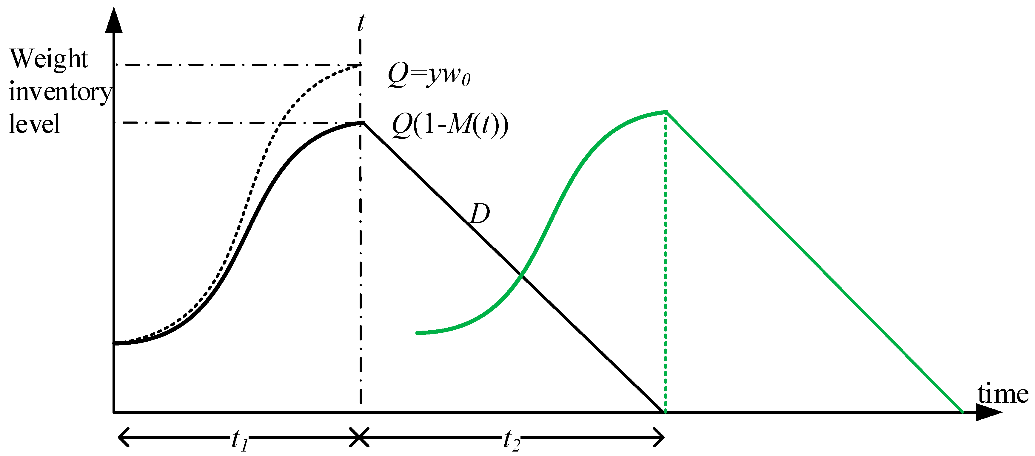
At the beginning of the breeding period ($t_1$) in the poultry farm, a lot of newborn birds $y$ with an initial weight $w_0$ (the weight of newborn birds) are purchased from suppliers and are then raised until they reach the market slaughter weight ($w_t$). Once the birds reach the proper size and weight, at the slaughter date ($t$), they are killed for market consumption annually. During the breeding period, several chickens are dead before reaching the slaughter date, mainly because they have reduced walking ability and due to lameness and reduced access to water and feed, which lead to debilitation and death. The number of dead birds at date $t$ is equal to $yM\left(t\right)$, where $M\left(t\right)$ is the percentage of the cumulative daily mortality. Therefore, on the slaughter date, the number of live birds $y\left(1-M\left(t\right)\right)$ are killed for consumption, and the rest of them, $yM\left(t\right)$, are disposed. After the slaughtering process, the consumption period ($t_2$) starts with the constant demand rate ($D$) until the weight inventory level reaches zero. The behavior of the weight inventory system of growing items is illustrated in Figure 1.

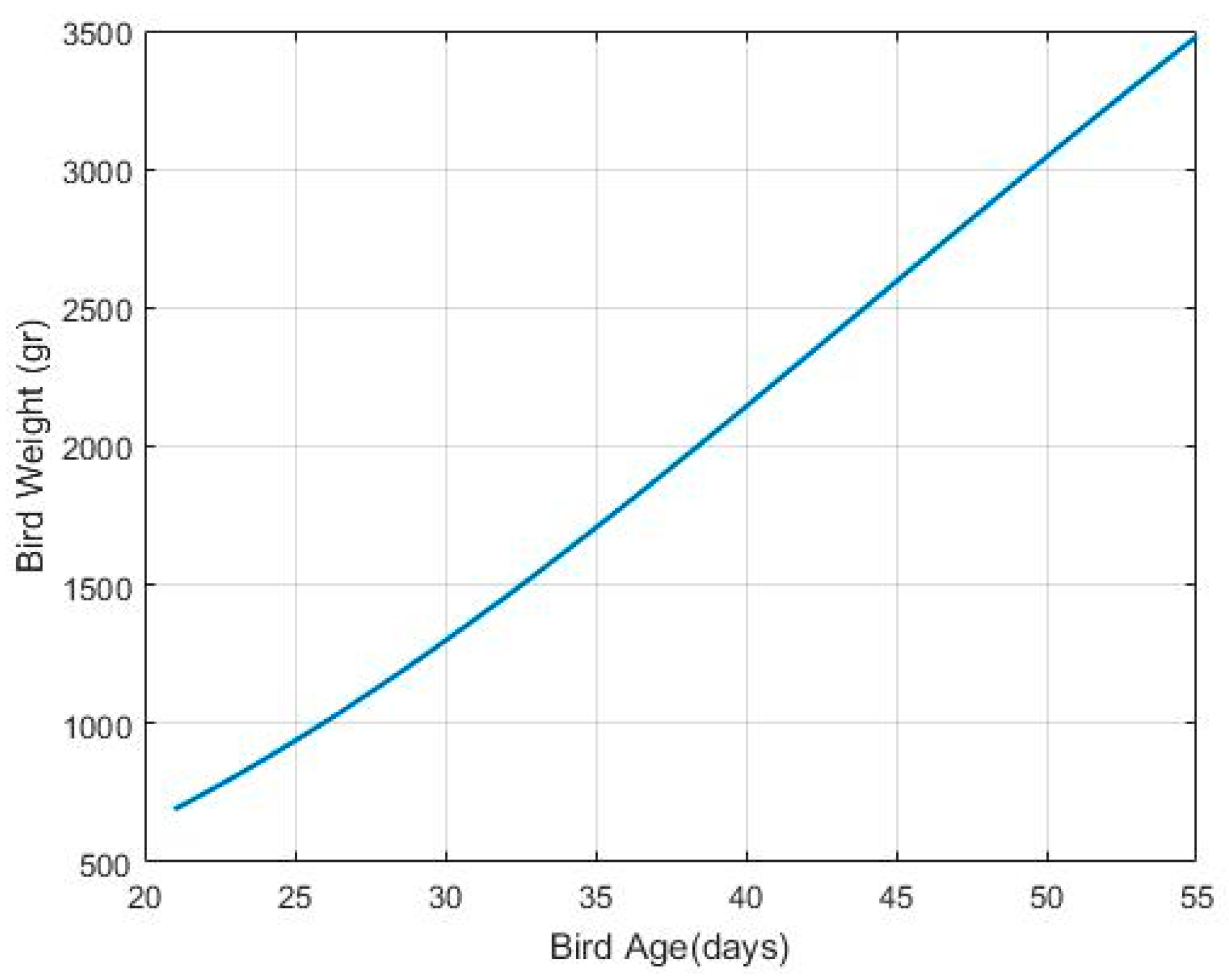
For the growth function, there are several valuable studies that have measured bird growth (Rezaei [6]); however, the Richards function, proposed by Richards [33], is one of the most important growth functions for bird weight (see also Goliomytis et al. [34]). Therefore, this function is used in this study, as follows:

$$w_t=A{\left(1+b{e}^{-kt}\right)}^{\raisebox{1ex}{$-1$}\!\left/ \!\raisebox{-1ex}{$n$}\right.}$$

(1)

where $w_t$ is the weight of the body of a live bird at age $t$.

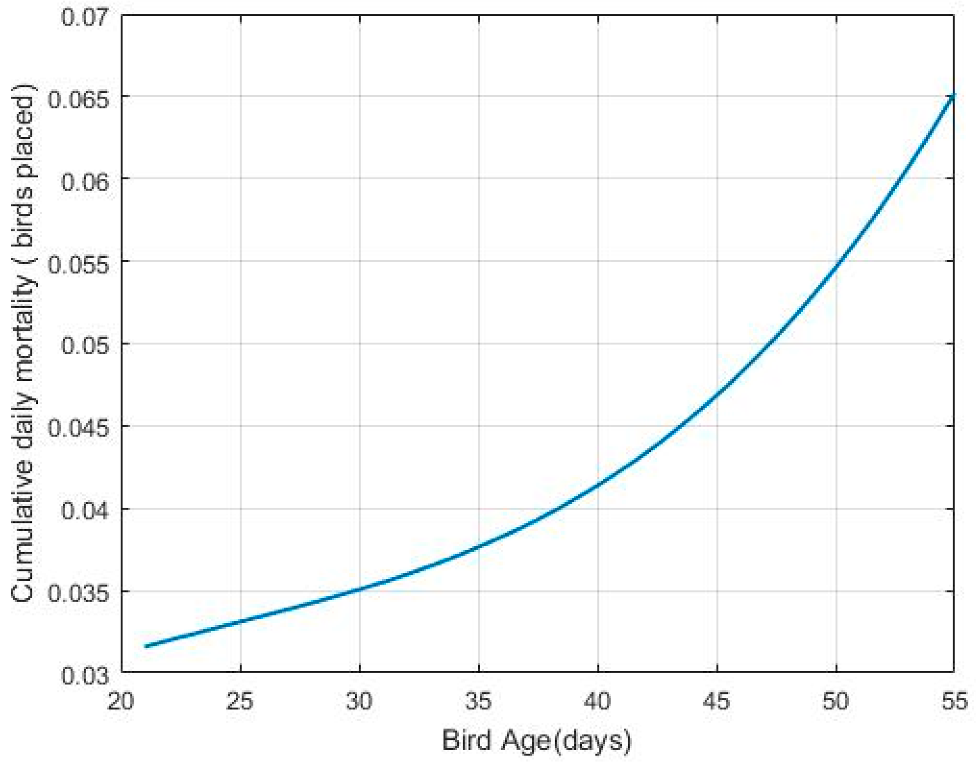
As mentioned before, many birds are dead during breeding. In the current study, we use the polynomial function of the percentage of cumulative daily mortality, which relates the percentage of daily mortality to the age of birds, based on the work of Xin et al. [35], as follows:

$$M\left(t\right)=m_0+m_{1}t+m_2{t}^2+m_3{t}^3$$

(2)

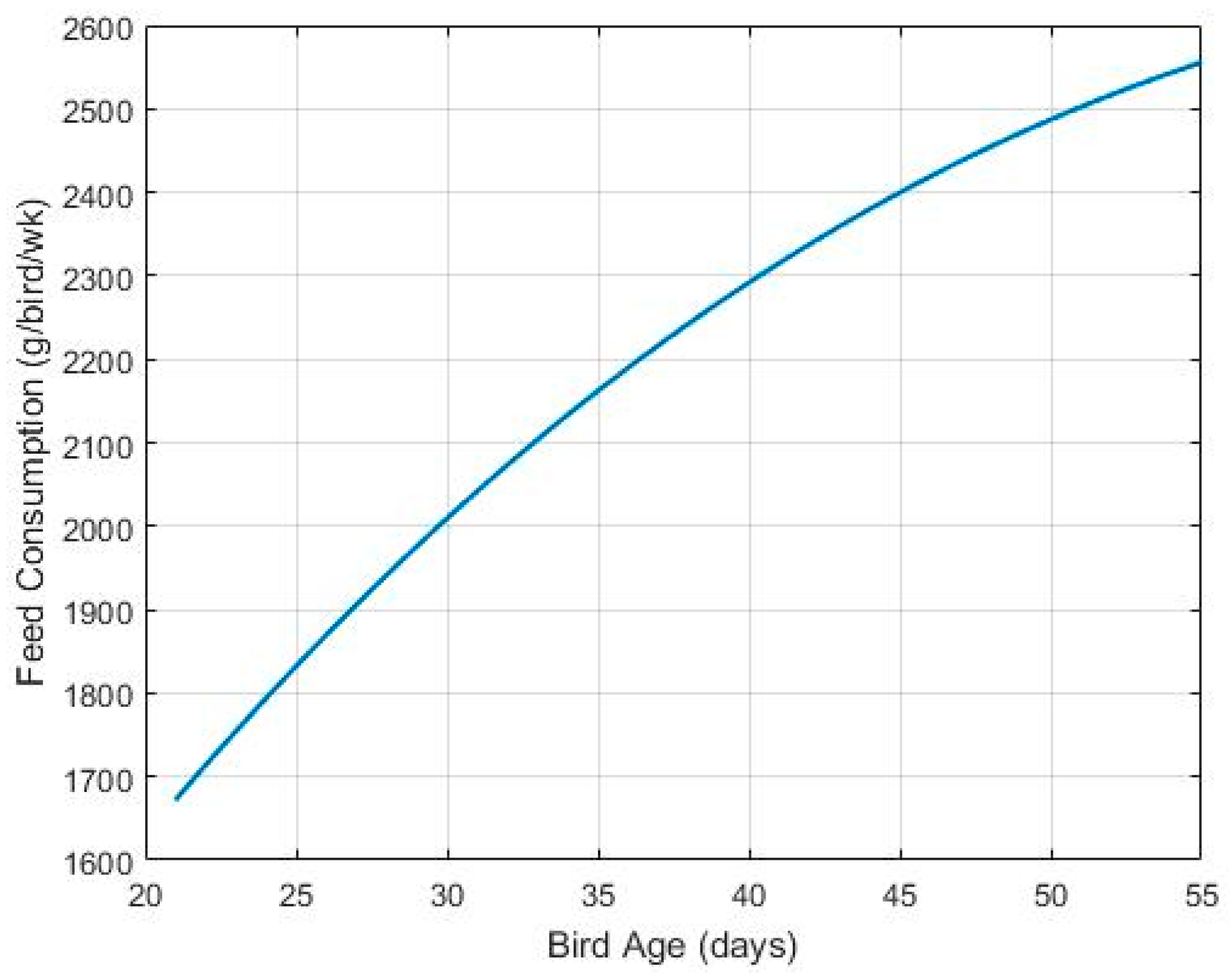
During the breeding period, birds grow and nurture with a feeding function, as presented by Goliomytis et al. [34]. This function is a polynomial function, which depends on the birds’ age. This function is fitted based on the collected data and is estimated as follows:

$$F\left(t\right)=f_0+f_{1}t+f_2{t}^2+f_3{t}^3$$

(3)

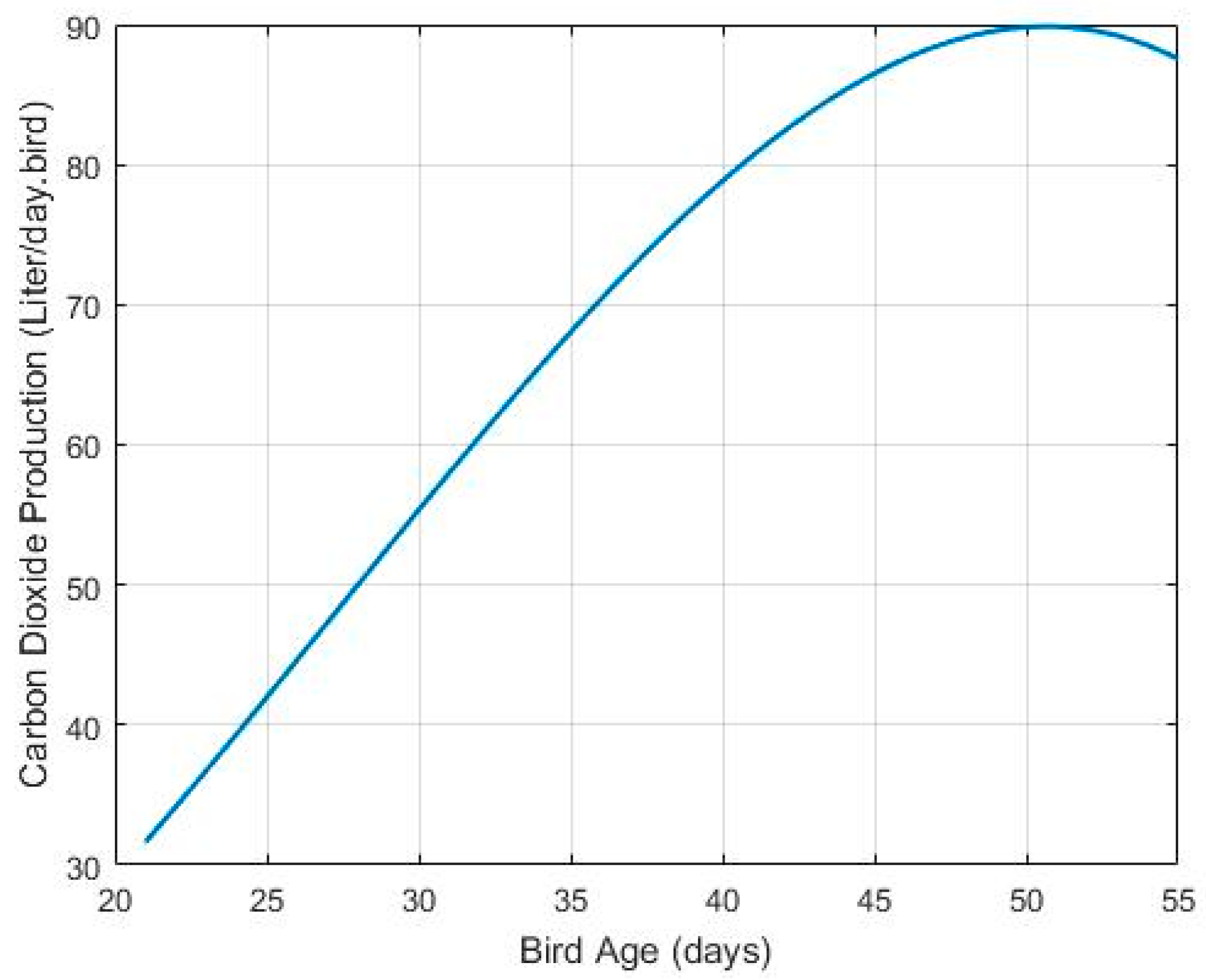
Moreover, for carbon dioxide production function, we choose the commonly polynomial function in the real world, which depends on the age of the birds, and it is fitted and estimated according to Leonard et al. [36], as follows:

$$C\left(t\right)=c_0+c_{1}t+c_2{t}^2+c_3{t}^3$$

(4)

3.2. Objective Function and Constraints

We consider a condition where a poultry farm purchases newborn birds, grows them up to the market slaughter weight, kills them and responds to customer demand. The total cost of the inventory system includes the setup cost, purchasing cost, holding cost, feeding (production) cost, disposal cost and carbon dioxide production tax. Next, each component of the total cost is obtained as follows:

-

Setup cost

At the beginning of the breeding cycle, some activities and processes, such as cleaning and maintenance, are needed to start the breeding process, and the costs of these activities are imposed as the setup cost ($K$) on the company for each cycle. Because we should obtain the setup cost for a year, we can divide the setup cost per cycle by $t_2$, as follows:

$$TS=\frac{K}{t_2}$$

(5)

where $t_2$ is the consumption period, which can be obtained from Equation (6).

$$t_2=\frac{y{w}_t\left(1-M\left(t\right)\right)}{D}$$

(6)

Considering $t_2$, the annual setup cost is as follows:

$$TS=\frac{DK}{y{w}_t\left(1-M\left(t\right)\right)}$$

(7)

-

Purchasing cost

As Figure 1 shows, at first, a number of newborn birds ($y$) with an initial weight ($w_0$) are received from the supplier, and subsequently, the purchasing cost per growth cycle becomes equal to $py{w}_0$, where $p$ is the purchasing cost per weight unit. Therefore, the annual purchasing cost is computed as follows:

$$TP=\frac{py{w}_0}{t_2}=\frac{Dp{w}_0}{w_t\left(1-M\left(t\right)\right)}$$

(8)

-

Holding cost

It is easy to derive from Figure 1 that the average weight of the inventory level during the consumption period is $y\left(1-M\left(t\right)\right)w_t/2$, and the length of the consumption period is $t_2$. The holding cost per cycle is $h{t}_{2}y\left(1-M\left(t\right)\right)w_t/2$, where $h$ is the annual inventory cost per weight unit. Therefore, the annual holding cost is calculated as follows:

$$TH=\frac{h{t}_{2}y\left(1-M\left(t\right)\right)w_t}{2t_2}=\frac{h}{2}y{w}_t\left(1-M\left(t\right)\right)$$

(9)

-

Disposal cost

Several birds are dead during the breeding process as result of losing their ability to walk, and the percentage of cumulative daily mortality at the slaughter date $t$ is $M\left(t\right)$. Hence, the total number of birds that die during the breeding period is equal to $yM\left(t\right)$, and subsequently, the disposal cost per cycle is computed by multiplying $yM\left(t\right)$ by $r$, where $r$ is the disposal cost of a dead bird. Finally, the annual disposal cost is obtained as follows:

$$TD=\frac{ryM\left(t\right)}{t_2}=\frac{DrM\left(t\right)}{w_t\left(1-M\left(t\right)\right)}$$

(10)

-

Feeding (production) cost

The feeding function per weight unit, which depends on the age of the chicken, is stated in Equation (3). Considering $z$ and $t_1$, the feeding cost per unit and the length of the breeding period, respectively, the total feeding cost per cycle is $ey{{\displaystyle \int }}_0^{t_1}F\left(t\right)\left(1-M\left(t\right)\right)dt$. Thus, the annual feeding cost is calculated as follows:

$$TF=\frac{ey{{\displaystyle \int }}_0^{t}F\left(t\right)\left(1-M\left(t\right)\right)dt}{t_2}=\frac{Dz{{\displaystyle \int }}_0^{t}F\left(t\right)\left(1-M\left(t\right)\right)dt}{w_t\left(1-M\left(t\right)\right)}$$

(11)

-

Carbon Dioxide Production Tax

According to Broucek and Cermák [37], CO₂ production by animals is relative to their metabolic heat production and consequently to their metabolic body weight, which, in turn, is affected by bird activity and temperature. Carbon dioxide is produced during the breeding process. The carbon dioxide production function, which depends on the birds’ age, is indicated in Equation (4). Considering $a$ and $t_1$, the tax cost of carbon dioxide production and the length of the breeding period, respectively, the annual tax of carbon dioxide production is obtained as follows:

$$TA=\frac{ay{{\displaystyle \int }}_0^{t}C\left(t\right)\left(1-M\left(t\right)\right)dt}{t_2}=\frac{Da{{\displaystyle \int }}_0^{t}C\left(t\right)\left(1-M\left(t\right)\right)dt}{w_t\left(1-M\left(t\right)\right)}$$

(12)

-

Total cost

The annual total cost is formulated as follows:

$$TC=\frac{DK}{y{w}_t\left(1-M\left(t\right)\right)}+\frac{h}{2}y{w}_t\left(1-M\left(t\right)\right)+\frac{D\left(p{w}_0+rM\left(t\right)\right)}{w_t\left(1-M\left(t\right)\right)}+\frac{Dz{{\displaystyle \int }}_0^{t}F\left(t\right)\left(1-M\left(t\right)\right)dt}{w_t\left(1-M\left(t\right)\right)}+\frac{Da{{\displaystyle \int }}_0^{t}C\left(t\right)\left(1-M\left(t\right)\right)dt}{w_t\left(1-M\left(t\right)\right)}$$

(13)

Substituting $w_t$ from Equation (1), the annual total cost is as follows:

$$\begin{array}{c}TC=\frac{DK}{yA{\left(1+b{e}^{-kt}\right)}^{-\raisebox{1ex}{$1$}\!\left/ \!\raisebox{-1ex}{$n$}\right.}\left(1-M\left(t\right)\right)}+\frac{h}{2}yA{\left(1+b{e}^{-kt}\right)}^{\raisebox{1ex}{$-1$}\!\left/ \!\raisebox{-1ex}{$n$}\right.}\left(1-M\left(t\right)\right)+\hfill \\ \frac{D\left(p{w}_0+rM\left(t\right)\right)}{A{\left(1+b{e}^{-kt}\right)}^{\raisebox{1ex}{$-1$}\!\left/ \!\raisebox{-1ex}{$n$}\right.}\left(1-M\left(t\right)\right)}+\frac{Dz{{\displaystyle \int }}_0^{t}F\left(t\right)\left(1-M\left(t\right)\right)dt}{A{\left(1+b{e}^{-kt}\right)}^{\raisebox{1ex}{$-1$}\!\left/ \!\raisebox{-1ex}{$n$}\right.}\left(1-M\left(t\right)\right)}+\frac{Da{{\displaystyle \int }}_0^{t}C\left(t\right)\left(1-M\left(t\right)\right)dt}{A{\left(1+b{e}^{-kt}\right)}^{-\raisebox{1ex}{$1$}\!\left/ \!\raisebox{-1ex}{$n$}\right.}\left(1-M\left(t\right)\right)}\hfill \end{array}$$

(14)

-

Constraints

When the company wants to order a number of newborn birds, the number of ordered items must be an integer number, as the company can buy only live birds. Moreover, the slaughter date must be an integer number between the minimum allowable length of the breeding period ($L$) and the maximum allowable length of it ($U$), because, in the real world, each domestic animal has a growth period that is determined by the market, breeding process and its nature. Therefore, this constraint is $L\le t\le U$.

-

Final Model

According to the objective function in Equation (14) and the constraints stated in the above subsection, the final model of the proposed study is as follows:

$$\begin{array}{c}Min TC=\frac{DK}{yA{\left(1+b{e}^{-kt}\right)}^{\raisebox{1ex}{$-1$}\!\left/ \!\raisebox{-1ex}{$n$}\right.}\left(1-M\left(t\right)\right)}+\frac{h}{2}yA{\left(1+b{e}^{-kt}\right)}^{\raisebox{1ex}{$-1$}\!\left/ \!\raisebox{-1ex}{$n$}\right.}\left(1-M\left(t\right)\right)+\hfill \\ \frac{D\left(p{w}_0+rM\left(t\right)\right)}{A{\left(1+b{e}^{-kt}\right)}^{\raisebox{1ex}{$-1$}\!\left/ \!\raisebox{-1ex}{$n$}\right.}\left(1-M\left(t\right)\right)}+\frac{Dz{{\displaystyle \int }}_0^{t}F\left(t\right)\left(1-M\left(t\right)\right)dt}{A{\left(1+b{e}^{-kt}\right)}^{\raisebox{1ex}{$-1$}\!\left/ \!\raisebox{-1ex}{$n$}\right.}\left(1-M\left(t\right)\right)}+\frac{Da{{\displaystyle \int }}_0^{t_1}C\left(t\right)\left(1-M\left(t\right)\right)dt}{A{\left(1+b{e}^{-kt}\right)}^{\raisebox{1ex}{$-1$}\!\left/ \!\raisebox{-1ex}{$n$}\right.}\left(1-M\left(t\right)\right)}\hfill \\ st: L\le t\le U\hfill \\ t,y>0 \& integer\hfill \end{array}$$

(15)

4. Solution Procedure and Numerical Example

At first, substituting $M\left(t\right)$, $F\left(t\right)$ and $C\left(t\right)$ from Equations (2)–(4), respectively, into the objective function Equation (15), the total cost is expressed as follows:

$$\begin{array}{c}TC=\frac{DK}{yA{\left(1+b{e}^{-kt}\right)}^{\raisebox{1ex}{$-1$}\!\left/ \!\raisebox{-1ex}{$n$}\right.}\left(1-\left(m_0+m_{1}t+m_2{t}^2+m_3{t}^3\right)\right)}+\frac{h}{2}yA{\left(1+b{e}^{-kt}\right)}^{\raisebox{1ex}{$-1$}\!\left/ \!\raisebox{-1ex}{$n$}\right.}(1-(m_0+m_{1}t+\hfill \\ m_2{t}^2+m_3{t}^3))+\frac{D\left(p{w}_0+r\left(m_0+m_{1}t+m_2{t}^2+m_3{t}^3\right)\right)}{A{\left(1+b{e}^{-kt}\right)}^{\raisebox{1ex}{$-1$}\!\left/ \!\raisebox{-1ex}{$n$}\right.}\left(1-\left(m_0+m_{1}t+m_2{t}^2+m_3{t}^3\right)\right)}+\hfill \\ \frac{Da{\alpha }_2\left(t\right)}{A{\left(1+b{e}^{-kt}\right)}^{\raisebox{1ex}{$-1$}\!\left/ \!\raisebox{-1ex}{$n$}\right.}\left(1-\left(m_0+m_{1}t+m_2{t}^2+m_3{t}^3\right)\right)}+\frac{Dz{\alpha }_1\left(t\right)}{A{\left(1+b{e}^{-kt}\right)}^{\raisebox{1ex}{$-1$}\!\left/ \!\raisebox{-1ex}{$n$}\right.}\left(1-\left(m_0+m_{1}t+m_2{t}^2+m_3{t}^3\right)\right)}\hfill \end{array}$$

(16)

where ${\alpha }_1\left(t\right)$ and ${\alpha }_2\left(t\right)$ are determined in Appendix A.

Next, we compute the partial derivation of the objective function (16) with respect to the slaughter date ($t$) and set it equal to zero, as follows:

$$\begin{array}{cc}\frac{\partial TC}{\partial t}=\hfill & \frac{DK{\left(b{e}^{-kt}+1\right)}^{\frac{1}{n}}\left(3m_3{t}^2+2m_{2}t+m_1\right)}{Ay{\left(m_3{t}^3+m_2{t}^2+m_{1}t+m_0-1\right)}^2}+\frac{DKbk{e}^{-kt}{\left(b{e}^{-kt}+1\right)}^{\frac{1}{n}-1}}{Any\left(m_3{t}^3+m_2{t}^2+m_{1}t+m_0-1\right)}-\frac{Ahy\left(3m_3{t}^2+2m_{2}t+m_1\right)}{2\ast {\left(b{e}^{-kt}+1\right)}^{\frac{1}{n}}}-\hfill \\ & \frac{Abhky{e}^{-kt}\left(m_3{t}^3+m_2{t}^2+m_{1}t+m_0-1\right)}{2n{\left(b{e}^{-kt}+1\right)}^{\frac{1}{n}+1}}+\hfill \\ & \frac{D\left(r\left(m_3{t}^3+m_2{t}^2+m_{1}t+m_0\right)+pw0\right){\left(b{e}^{-kt}+1\right)}^{\frac{1}{n}}\left(3m_3{t}^2+2m_{2}t+m_1\right)}{\left(A{\left(m_3{t}^3+m_2{t}^2+m_{1}t+m_0-1\right)}^2\right)}-\hfill \\ & \frac{Dr{\left(b{e}^{-kt}+1\right)}^{\frac{1}{n}}\left(3m_3{t}^2+2m_{2}t+m_1\right)}{\left(A\left(m_3{t}^3+m_2{t}^2+m_{1}t+m_0-1\right)\right)}+\frac{Dbk{e}^{-kt}\left(r\left(m_3{t}^3+m_2{t}^2+m_{1}t+m_0\right)+p{w}_0\right){\left(b{e}^{-kt}+1\right)}^{\frac{1}{n}-1}}{\left(An\left(m_3{t}^3+m_2{t}^2+m_{1}t+m_0-1\right)\right)}+\hfill \\ & {\beta }_1\left(t\right)+{\beta }_1\left(t\right)=0\hfill \end{array}$$

(17)

where ${\beta }_1\left(t\right)$ and ${\beta }_2\left(t\right)$ are determined in Appendix B.

The lives of animals are cut extremely short within industrial agriculture scenarios. Slaughter plants can kill animals in a limited predetermined age range. Therefore, if the length of the slaughter date is known, the objective function (17) only has one decision variable ($y$). As a result, the objective function ($T{C}^{\prime }$), which depends on the value of $y$, is expressed as follows:

$$\begin{array}{cc}T{C}^{\prime }=\hfill & \frac{DK}{yA{\left(1+b{e}^{-kt}\right)}^{\raisebox{1ex}{$-1$}\!\left/ \!\raisebox{-1ex}{$n$}\right.}\left(1-\left(m_0+m_{1}t+m_2{t}^2+m_3{t}^3\right)\right)}+\frac{h}{2}yA{\left(1+b{e}^{-kt}\right)}^{\raisebox{1ex}{$-1$}\!\left/ \!\raisebox{-1ex}{$n$}\right.}(1-(m_0+m_{1}t+\\ & m_2{t}^2+m_3{t}^3\left)\right)\hfill \end{array}$$

(18)

Based on the study of García-Laguna et al. [38], the optimal integer value of each objective function as ${\Delta }_1/y+{\Delta }_{2}y; {\Delta }_1.{\Delta }_2>0$ is $y=\lceil -0.5+\sqrt{0.25+{\Delta }_1/{\Delta }_2}\rceil$, where $\lceil y\rceil$ is the biggest integer number of $y$, i.e., $\lceil 2.5\rceil =3$. Therefore, the optimal integer number of newborn animals ordered is as follows:

$$y=\lceil -0.5+\sqrt{0.25+\frac{2DK}{A^2{\left(1+b{e}^{-kt}\right)}^{\raisebox{1ex}{$-2$}\!\left/ \!\raisebox{-1ex}{$n$}\right.}{\left(1-\left(m_0+m_{1}t+m_2{t}^2+m_3{t}^3\right)\right)}^2}}\rceil$$

(19)

Then, the optimal number of newborn items ordered is determined using Equation (19) with respect to the constraints of Equation (15). Finally, the steps of the proposed solution procedure are as follows:

Step 1. For t = L, $L+1$, …, $U$

(a)

Calculate the optimal number of y(t) using Equation (19).

(b)

Determine the optimal value of $T{C}^{\ast }\left(t\right)$ from Equation (16).

Step 2. Compare all $T{C}^{\ast }\left(t\right)$ for $t=L$, $L+1$, …, $U$. The pair ($t.y$(t)) is the optimal solution of the problem that provides the lowest cost.

Numerical Example

We present a numerical example for a specific type of inventory system with fast-growing birds, male broilers, to illustrate the proposed model. The lives of broiler chickens are cut extremely short within industrial agriculture scenarios. Slaughter plants can kill broilers from 21 days to 170 days old. However, the usual slaughter age is 47 days in the US, whereas the slaughter age is 42 days in European countries (European Food Safety Authority, [39]). Therefore, the values of the minimum ($L$) and maximum ($U$) allowable length of the breeding period are 21 and 55, to make a practical model. We use the parameters of Richard’s growth curve and the feed consumption curve estimated by Goliomytis et al. [34], as follows:

$$n=0.0087; b=0.043;A=6870.2; k=0.036, \mathrm{and}$$

$$f_0=532.2; f_1=67.15; f_2=-0.651; f_3=0.0018$$

As a result, the growth curve and the feed consumption curve are applied for this instance, as follows (see Figure 2 and Figure 3):

$$w_t=6870.2{\left(1+0.043e^{-0.036t}\right)}^{\raisebox{1ex}{$-1$}\!\left/ \!\raisebox{-1ex}{$0.0087$}\right.}; \mathrm{and} F\left(t\right)=532.2+67.15t-0.651t^2+0.0018t^3$$

For the mortality function, we use the polynomial function $M\left(t\right)$ with the following parameters, which are the same as those used by Xin et al. [35]:

$$m_0=0.0126; m_1=0.00174; m_2=-0.0000556; m_3=0.000000753$$

Thus, the mortality curve is (see Figure 4)

$$M\left(t\right)=0.0126+0.00174t-0.0000556t^2+0.000000753t^3.$$

Additionally, we apply the polynomial function $C\left(t\right)$ for carbon dioxide production (liter/day.bird) with the following parameters based on the work of Leonard et al. [36]:

$$c_0=8.16; c_1=-0.9768; c_2=0.13416; c_3=-0.0016392.$$

Consequently, the carbon dioxide production curve is as follows (see Figure 5):

$$C\left(t\right)=8.16-0.9768t+0.13416t^2-0.0016392t^3.$$

All the parameters of the above growth, feed consumption, mortality and carbon dioxide production curve functions were estimated based on the real cases for broilers in the works of Richard [33], Goliomytis et al. [34], Xin et al. [35] and Leonard et al. [36], respectively.

We assume that the rest of the parameters of the inventory system are as follows:

$$\begin{gathered} w_0=45 \mathrm{g}; h=0.002 \$/\mathrm{year}; D=100,000,000 \mathrm{g}; z=0.0001 \$/\mathrm{g}/\mathrm{day}; K= \\ 5000 \$/\mathrm{cycle}; p=0.01 \$/\mathrm{g}; a=0.001 \$/\mathrm{L}/\mathrm{d}·\mathrm{g}; \mathrm{and} r=1 \$/\mathrm{bird} \end{gathered}$$

Based on the proposed solution method, the optimal value of the slaughter age is $t^{\ast }=44$ (see Figure 6). Then, substituting $t^{\ast }$ into Equations (16) and (19), the other optimal results are determined, as follows: $y^{\ast }=419$ newborn chickens, and $T{C}^{\ast }=878991.3$ USD.

5. Sensitivity Analysis and Managerial Insights

In this section, we consider all the cost parameters of the proposed model and the initial weight as relevant variables for a sensitivity analysis. These parameters include the holding cost, the setup cost, the initial weight of the chick, the feeding cost, the purchasing cost, the tax on carbon dioxide production and the disposal cost per carcass.

Table 2. Sensitivity analysis of the holding cost ($h$).

% Changes	$\mathit{T}{\mathit{C}}^{\ast }$	${\mathit{y}}^{\ast }$	${\mathit{t}}^{\ast }$
−90	878,090	419	44
−70	878,290	419	44
−50	878,490	419	44
−30	878,691	419	44
−10	878,891	419	44
0	878,991	419	44
10	879,091	419	44
30	879,291	419	44
50	879,491	419	44
70	879,692	419	44
90	879,892	419	44

,

Table 3. Sensitivity analysis of the setup cost ($K$).

% Changes	$\mathit{T}{\mathit{C}}^{\ast }$	${\mathit{y}}^{\ast }$	${\mathit{t}}^{\ast }$
−90	536,545	124	46
−70	652,210	222	45
−50	732,363	277	46
−30	797,899	363	43
−10	853,314	384	45
0	878,991	419	44
10	903,229	411	46
30	949,552	495	43
50	991,671	513	44
70	1,031,425	546	44
90	1,068,361	540	46

,

Table 4. Sensitivity analysis of the initial weight ($w_0$).

% Changes	$\mathit{T}{\mathit{C}}^{\ast }$	${\mathit{y}}^{\ast }$	${\mathit{t}}^{\ast }$
−90	861,989	434	43
−70	865,806	419	44
−50	869,573	419	44
−30	873,340	419	44
−10	877,107	419	44
0	878,991	419	44
10	880,874	419	44
30	884,641	419	44
50	888,207	368	48
70	891,519	368	48
90	894,793	348	50

,

Table 5. Sensitivity analysis of the feeding cost ($z$).

% Changes	$\mathit{T}{\mathit{C}}^{\ast }$	${\mathit{y}}^{\ast }$	${\mathit{t}}^{\ast }$
−90	617,673	508	39
−70	676,195	419	44
−50	734,137	419	44
−30	792,078	419	44
−10	850,020	419	44
0	878,991	419	44
10	907,962	419	44
30	965,903	419	44
50	1,023,845	419	44
70	1,081,786	419	44
90	1,139,601	368	48

,

Table 6. Sensitivity analysis of the purchasing cost ($p$).

% Changes	$\mathit{T}{\mathit{C}}^{\ast }$	${\mathit{y}}^{\ast }$	${\mathit{t}}^{\ast }$
−90	861,989	434	43
−70	865,806	419	44
−50	869,573	419	44
−30	873,340	419	44
−10	877,107	419	44
0	878,991	419	44
10	880,874	419	44
30	884,641	419	44
50	888,207	368	48
70	891,519	368	48
90	894,793	348	50

,

Table 7. Sensitivity analysis of the tax of CO₂ production ($a$).

% Changes	$\mathit{T}{\mathit{C}}^{\ast }$	${\mathit{y}}^{\ast }$	${\mathit{t}}^{\ast }$
−90	814,140	348	50
−70	828,934	348	50
−50	843,729	348	50
−30	858,309	368	48
−10	872,185	419	44
0	878,991	419	44
10	885,797	419	44
30	899,408	419	44
50	913,020	419	44
70	926,387	468	41
90	939,369	468	41

and

Table 8. Sensitivity analysis of the disposal cost ($r$).

% Changes	$\mathit{T}{\mathit{C}}^{\ast }$	${\mathit{y}}^{\ast }$	${\mathit{t}}^{\ast }$
−90	877,271	419	44
−70	877,653	419	44
−50	878,035	419	44
−30	878,417	419	44
−10	878,800	419	44
0	878,991	419	44
10	879,182	419	44
30	879,564	419	44
50	879,946	419	44
70	880,329	419	44
90	880,711	419	44

show the effects of the parameters on the optimal value of the objective function, the order quantity and the slaughter age. Moreover, the effects of the parameter’s fluctuations on the optimal value of $T{C}^{\ast }$, $y^{\ast }$ and $t^{\ast }$ are depicted in Figure 7, Figure 8 and Figure 9.

As illustrated in Figure 7, the optimal total cost increases if the value of the feeding, setup and carbon dioxide production costs increase; however, it is highly sensitive to changes in the value of the feeding cost and the setup cost. Additionally, the optimal objective function is slightly sensitive to changes in the other parameters; however, if they increase, there is an increasing trend for the objective function.

According to Figure 8, we can state that the optimal order quantity of newborn chicks is highly sensitive to fluctuations in the value of the setup cost. On the other hand, this quantity is not affected by the holding cost and/or the disposal cost. However, the value of the optimal order quantity decreases if the value of the feeding cost, the initial weight and/or the purchasing cost increases.

Finally, on the one hand, as shown in Figure 9, the optimal slaughter age decreases if the value of the tax of carbon dioxide production increases; on the other hand, it increases if the value of the purchasing cost and the initial weight increases. The duration of the birds’ age is not notably affected by the feeding cost and setup cost. Moreover, this optimal age is not sensitive to fluctuations in the value of the disposal cost and the holding cost.

Moreover, Table 3 shows that the setup cost (K) is imposed on the total cost in each cycle and is not related to the order quantity. Therefore, as this cost goes up, so does the number of chicks ordered because the model prefers to buy more chicks in each order to find a balance between variable and fixed costs. However, this cost has no significant effect on the breeding time. On the other hand, as shown in Table 6, the purchase price (p) is related to the order quantity of newborn chicks, so if this cost increases, the system tries to purchase fewer newborn items. Because the weight of chicks depends on how long it takes to raise them, the system increases the breeding period to meet more demand. Moreover, the carbon dioxide tax (a) and the chicks’ age are related together based on Table 7. Thus, if the government increases the carbon dioxide tax, the company can try to purchase more newborn chicks but breed them in less time so that the total cost is minimized.

5.1. Managerial Insights

The proposed model investigates the effects of growing items on the EOQ problem; therefore, it can help companies to estimate the space of the breeding salon with respect to the number of ordered newborn chicks and the weight of birds when they are supposed to be slaughtered. Moreover, the required budget per cycle is computed by multiplying the optimal initial purchase volume ($y{w}_0$) by the purchasing cost per weight ($p$). The model can easily estimate the running costs of a farming company. As stated, the goal of this growing inventory model is to obtain the optimal slaughter age and the optimal number of newborn chicks, purchased from the supplier, to minimize the total costs.

One way to get managers to reduce their carbon footprint is to add the cost of carbon emissions to the total cost of the inventory management system; see, for example, the work of Nobil et al. [39]. Carbon dioxide emissions are one of the most important issues covered by this study. Carbon dioxide production is assumed to be a polynomial function that relates CO₂ production to the age of the birds. Based on this practical function, it is simple to calculate the amount of carbon dioxide production emitted by a company, and managers can then compute the associated costs because the government usually determines a tax for each ton of carbon dioxide produced. Furthermore, to make the EOQ problem with growing items more practical, this study constructs a solution procedure to obtain a discrete number of newborn chicks. This issue was not considered in the solution procedure proposed by Rezaei [6].

This study also investigates the effects of the disposal cost of carcasses during the growth period. The number of dead chickens is calculated with a practical polynomial function that depends on how old the chickens are. Therefore, based on how old the chickens are, managers can determine how many of them die in each cycle and then take the steps needed to get rid of their bodies. As can be seen in Table 8, the total cost increases if the disposal cost per carcass increases, so the government can help companies destroy the carcasses with financial support packages to prevent any illegal disposal methods. If the disposal cost of carcasses is high, some companies may use illegal methods, which have harmful effects on the environment and thus endanger the health of humans and animals. Some of these illegal methods are: (I) using excessive additives, antibiotics, hormones and drugs to prevent the deaths of the birds or to increase their growth rate and weight gain; (II) selling carcasses to factories that manufacture processed meat “sausages”, as buying carcasses is cheaper than buying live birds; (III) selling carcasses to companies that raise other animals, such as pigs, who use them as a cheaper alternative to feed their animals; and (IV) dumping carcasses into places such as wells and rivers or with improper burial options in the soil. The government can help companies with a financial support package or offer a proper disposal method to destroy the carcasses that were produced during the growth cycle. It was discovered that the death rate of the living items has a considerable impact on corporate performance. In general, profit increases as the mortality rate falls. Therefore, management should take steps to maintain the lowest feasible death rates.

5.2. Discussion

In this proposed model, if the assumption of the number of orders, which is supposed to be an integer, is not considered, the proposed MINLP model becomes a nonlinear programming (NLP) model. Therefore, instead of Equation (19), we can determine the number of newborn chicks from Equation (20). However, if we do not stick to this assumption, the answer to the NLP model does not fit the real world because the number of ordered chickens cannot be a continuous number.

$$y=\frac{2DK}{A^2{\left(1+b{e}^{-kt}\right)}^{\raisebox{1ex}{$-2$}\!\left/ \!\raisebox{-1ex}{$n$}\right.}{\left(1-\left(m_0+m_{1}t+m_2{t}^2+m_3{t}^3\right)\right)}^2}$$

(20)

In addition, if the carbon dioxide tax and the mortality function are not taken into account, the proposed model of the current study approximates the mathematical model of Rezaei [6]. However, if we disregard the carbon dioxide tax, the proposed model becomes the model of Sebatjane and Adetunji [25], approximately.

6. Conclusions

CO₂ emissions trap heat close to the Earth and, as a result, change the global climate. Therefore, reducing CO₂ emissions is vital, so their effects are mitigated. A significant reduction promotes some benefits, such as decreasing the global climate temperature, improving public health and boosting the global economy. If carbon emissions decrease, we can benefit from cleaner food, water and air. As a contribution to this goal, this study proposes an economic growth quantity model for fast-growing animals under a sustainable green breeding policy. Carbon dioxide production is modeled as a practical polynomial function that relates to the age of the birds. We also use another polynomial function to determine the number of dead chickens in the growth cycle. Taking into consideration carcasses is important due to two major causes: breeding and disposal costs. Thus, the proposed mathematical model is formulated as an integer nonlinear programming problem for a growing inventory system with mortality and CO₂ production. The objective function minimizes the total inventory cost, which includes the setup, the purchasing, the holding, the feed (production) and the disposal costs, as well as the CO₂ production tax, to determine the optimal slaughter age of the birds and the optimal order quantity for newborn chicks. Last, to find the best solutions, we use a proposed analytical method with a few simple steps.

We can extend the proposed inventory model by (I) considering food supply chains for the system, (II) assuming budget and warehouse space constraints for purchasing newborn chicks and their breeding, (III) allowing the occurrence of shortages in the consumption period, (IV) producing several types of animals, such as pigs, ducks and turkeys, (V) deteriorating slaughtered items during the consumption period, (VI) shipping the slaughtered items to the retailer via discrete shipments, (VII) regarding the mathematical model’s uncertainty parameters, such as demand and price, and (VIII) considering this model under permissible delays in payments.

References

1. Nobil, A.; Taleizadeh, A.A. Economic order quantity for growing items with discrete orders. J. Model. Eng. 2019, 17, 123–129. [Google Scholar]
2. Pasandideh, S.H.R.; Niaki, S.T.A.; Nobil, A.H.; Cárdenas-Barrón, L.E. A multiproduct single machine economic production quantity model for an imperfect production system under warehouse construction cost. Int. J. Prod. Econ. 2015, 169, 203–214. [Google Scholar] [CrossRef]
3. MacLeod, M.; Leinonen, I.; Wall, E.; Houdijk, J.; Eory, V.; Burns, J.; Ahmad, B.V.; Gómez-Barbero, M. Impact of Animal Breeding on GHG Emissions and Farm Economics; Publications Office of the European Union: Luxembourg, 2019. [Google Scholar]
4. Cockram, M.S.; Dulal, K.J. Injury and mortality in broilers during handling and transport to slaughter. Can. J. Anim. Sci. 2018, 98, 416–432. [Google Scholar] [CrossRef] [Green Version]
5. Nobil, A.H.; Nobil, E.; Sarker, B.R. Optimal decision-making for a single-stage manufacturing system with rework options. Int. J. Syst. Sci. Oper. Logist. 2020, 7, 90–104. [Google Scholar] [CrossRef]
6. Rezaei, J. Economic order quantity for growing items. Int. J. Prod. Econ. 2014, 155, 109–113. [Google Scholar] [CrossRef]
7. Liu, Z.; Lang, L.; Hu, B.; Shi, L.; Huang, B.; Zhao, Y. Emission reduction decision of agricultural supply chain considering carbon tax and investment cooperation. J. Clean. Prod. 2021, 294, 126305. [Google Scholar] [CrossRef]
8. Almeida, C.M.V.B.; Onilla, S.H.; Iannetti, B.F.; Huisingh, D. Cleaner production initiatives and challenges for a sustainable world: An introduction to this special volume. J. Clean. Prod. 2013, 47, 1–10. [Google Scholar] [CrossRef]
9. Nobil, A.H.; Sedigh, A.H.A.; Cárdenas-Barrón, L.E. A generalized economic order quantity inventory model with shortage: Case study of a poultry farmer. Arab. J. Sci. Eng. 2019, 44, 2653–2663. [Google Scholar] [CrossRef]
10. Khalilpourazari, S.; Pasandideh, S.H.R. Modeling and optimization of multi-item multi-constrained EOQ model for growing items. Knowl.-Based Syst. 2019, 164, 150–162. [Google Scholar] [CrossRef]
11. Sebatjane, M.; Adetunji, O. Economic order quantity model for growing items with imperfect quality. Oper. Res. Perspect. 2019, 6, 100088. [Google Scholar] [CrossRef]
12. Alfares, H.K.; Afzal, A.R. An economic order quantity model for growing items with imperfect quality and shortages. Arab. J. Sci. Eng. 2021, 46, 1863–1875. [Google Scholar] [CrossRef]
13. Mokhtari, H.; Salmasnia, A.; Asadkhani, J. A new production-inventory planning model for joint growing and deteriorating items. Int. J. Supply Oper. Manag. 2020, 7, 1–16. [Google Scholar]
14. Pourmohammad-Zia, N.; Karimi, B. Optimal replenishment and breeding policies for growing items. Arab. J. Sci. Eng. 2020, 45, 7005–7015. [Google Scholar] [CrossRef]
15. Sebatjane, M.; Adetunji, O. Economic order quantity model for growing items with incremental quantity discounts. J. Ind. Eng. Int. 2019, 15, 545–556. [Google Scholar] [CrossRef] [Green Version]
16. Hidayat, Y.A.; Riaventin, V.N.; Jayadi, O. Economic order quantity model for growing items with incremental quantity discounts, capacitated storage facility, and limited budget. J. Tek. Ind. 2020, 22, 1–10. [Google Scholar] [CrossRef]
17. Sebatjane, M.; Adetunji, O. Three-echelon supply chain inventory model for growing items. J. Model. Manag. 2019, 15, 567–587. [Google Scholar] [CrossRef]
18. Pourmohammad-Zia, N. A review of the research developments on inventory management of growing items. J. Supply Chain. Manag. Sci. 2021, 2, 71–84. [Google Scholar]
19. Pourmohammad-Zia, N.; Karimi, B.; Rezaei, J. Dynamic pricing and inventory control policies in a food supply chain of growing and deteriorating items. Ann. Oper. Res. 2021, 1–40. [Google Scholar] [CrossRef]
20. Mahato, C.; De, S.K.; Mahata, G.C. Joint pricing and inventory management for growing items in a supply chain under trade credit. Soft Comput. 2021, 25, 7271–7295. [Google Scholar] [CrossRef]
21. Malekitabar, M.; Yaghoubi, S.; Gholamian, M.R. A novel mathematical inventory model for growing-mortal items (case study: Rainbow trout). Appl. Math. Model. 2019, 71, 96–117. [Google Scholar] [CrossRef]
22. Sebatjane, M.; Adetunji, O. A three-echelon supply chain for economic growing quantity model with price-and freshness-dependent demand: Pricing, ordering and shipment decisions. Oper. Res. Perspect. 2020, 7, 100153. [Google Scholar] [CrossRef]
23. Sebatjane, M.; Adetunji, O. Optimal inventory replenishment and shipment policies in a four-echelon supply chain for growing items with imperfect quality. Prod. Manuf. Res. 2020, 8, 130–157. [Google Scholar] [CrossRef]
24. Sebatjane, M.; Adetunji, O. Optimal lot-sizing and shipment decisions in a three-echelon supply chain for growing items with inventory level- and expiration date-dependent demand. Appl. Math. Model. 2021, 90, 1204–1225. [Google Scholar] [CrossRef]
25. Sebatjane, M.; Adetunji, O. Optimal inventory replenishment and shipment policies in a three-echelon supply chain for growing items with expiration dates. Opsearch 2022, 59, 809–838. [Google Scholar] [CrossRef]
26. Gharaei, A.; Almehdawe, E. Economic growing quantity. Int. J. Prod. Econ. 2020, 223, 107517. [Google Scholar] [CrossRef]
27. Zhang, Y.; Li, L.Y.; Tian, X.Q.; Feng, C. Inventory management research for growing items with carbon-constrained. In Proceedings of the 2016 35th Chinese Control Conference (CCC), Chengdu, China, 27–29 July 2016; pp. 9588–9593. [Google Scholar]
28. De-la-Cruz-Márquez, C.G.; Cárdenas-Barrón, L.E.; Mandal, B. An inventory model for growing items with imperfect quality when the demand is price sensitive under carbon emissions and shortages. Math. Probl. Eng. 2021, 2021, 1–23. [Google Scholar] [CrossRef]
29. De-la-Cruz-Márquez, C.G.; Cárdenas-Barrón, L.E.; Mandal, B.; Smith, N.R.; Bourguet-Díaz, R.E.; Loera-Hernández, I.D.J.; Céspedes-Mota; Treviño-Garza, G. An inventory model in a three-echelon supply chain for growing items with imperfect quality, mortality, and shortages under carbon emissions when the demand is price sensitive. Mathematics 2022, 10, 4684. [Google Scholar] [CrossRef]
30. Choudhury, M.; Mahata, G.C. Sustainable integrated and pricing decisions for two-echelon supplier–retailer supply chain of growing items. RAIRO-Oper. Res. 2021, 55, 3171–3195. [Google Scholar] [CrossRef]
31. Rana, K.; Singh, S.R.; Saxena, N.; Sana, S.S. Growing items inventory model for carbon emission under the permissible delay in payment with partially backlogging. Green Financ. 2021, 3, 153–174. [Google Scholar] [CrossRef]
32. Gharaei, A.; Almehdawe, E. Optimal sustainable order quantities for growing items. J. Clean. Prod. 2021, 307, 127216. [Google Scholar] [CrossRef]
33. Richards, F.J. A Flexible Growth Function for Empirical Use. J. Exp. Bot. 1959, 10, 290–301. [Google Scholar] [CrossRef]
34. Goliomytis, M.; Panopoulou, E.; Rogdakis, E. Growth curves for body weight and major component parts, feed consumption, and mortality of male broiler chickens raised to maturity. Poult. Sci. 2003, 82, 1061–1068. [Google Scholar] [CrossRef] [PubMed]
35. Xin, H.; Berry, I.L.; Barton, T.L.; Tabler, G.T. Feed and water consumption, growth, and mortality of male broilers. Poult. Sci. 1994, 73, 610–616. [Google Scholar] [CrossRef] [PubMed]
36. Leonard, J.J.; Feddes, J.J.R.; McQuitty, J.B. Air quality in commercial broiler housing. Can Agric. Eng. 1984, 26, 65–72. [Google Scholar]
37. Broucek, J.; Cermák, B. Emission of harmful gases from poultry farms and possibilities of their reduction. Ekologia 2015, 34, 89. [Google Scholar] [CrossRef] [Green Version]
38. García-Laguna, J.; San-José, L.A.; Cárdenas-Barrón, L.E.; Sicilia, J. The integrality of the lot size in the basic EOQ and EPQ models: Applications to other production-inventory models. Appl. Math. Comput. 2010, 216, 1660–1672. [Google Scholar] [CrossRef]
39. European Food Safety Authority. Update on the state of play of animal health and welfare and environmental impact of animals derived from SCNT cloning and their offspring, and food safety of products obtained from those animals. EFSA J. 2012, 10, 2794. [Google Scholar]
Figure 1. The weight inventory level graph of growing items.
Mathematics 11 01039 g001
Figure 2. Weight growth curve.
Mathematics 11 01039 g002
Figure 3. Feed consumption curve.
Mathematics 11 01039 g003
Figure 4. Cumulative daily mortality curve.
Mathematics 11 01039 g004
Figure 5. Carbon dioxide production curve.
Mathematics 11 01039 g005
Figure 6. The value of the objective function regarding slaughter age.
Mathematics 11 01039 g006
Figure 7. The effects of the parameter’s fluctuations on the optimal value of the total cost.
Mathematics 11 01039 g007
Figure 8. The effects of the parameter’s fluctuations on the optimal value of the order quantity.
Mathematics 11 01039 g008
Figure 9. The effects of the parameter’s fluctuations on the optimal value of the slaughter age.
Mathematics 11 01039 g009