1. Introduction
The number of tardy jobs is a fundamental criterion related to the due date in scheduling problems. It is critical for examining the efficiency of production and evaluation management and has a wide range of applications in reality. The weighted number of tardy jobs is a familiar scheduling criterion in scheduling research. The objective function
was first studied by Moore [
1] and then,
was studied in many works, among which Lawler and Moore [
2], Karp [
3], and Sahni [
4] are representative. Subsequently, more and more studies on these two objectives were presented, especially the primary–secondary scheduling problems and the multi-agent scheduling problems, which can better meet the needs of customers and managers. In the previous multi-criterion scheduling problems, each of the jobs to be scheduled generally had a single weight. However, there are cases in which the jobs have multi-weights.
Take the information transmission as an example. In computer systems, information transmission is an important and common business. In practice, an information service company would transmit n pieces of information (corresponding to n jobs ) to m customers (where ) every day. Each piece of information has its own transmission time (corresponding to the processing time of ), which may be different on different days. Based on the usual cooperation experience, all the m customers have an expected time for receiving each information (corresponding to the due date of ). The transmission time of each piece of information on each workday is known in advance. In addition, the importance of each piece of information to different customers is different. So each piece of information will have m weights (), called the weight vector of , where is the weight of with respect to the i-th customer and also can be understood as the degree of dissatisfaction of the i-th customer when is tardy. The information service company definitely hopes all the customers can receive all the information on time, but sometimes this is impractical. Therefore, the decision maker needs to find a reasonable information transmission scheme to minimize all the customers’ degrees of dissatisfaction, or equivalently, to minimize the sum of the weight vectors of the tardy jobs, which is called the objective vector. Considering the conflicts of interest and inconsistencies between different customers, finding all the non-dominated solutions is an ideal choice to the problem. This motivates us to study the problem in this paper.
For the sake of understanding the problem better, now let us consider a concrete instance with
and
. The data are given in the following
Table 1.
In this instance, there are many ways to schedule the jobs, and the objective weight vectors maybe different for different schedules. In the following
Figure 1,
Figure 2 and
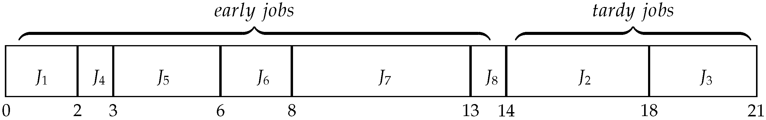
Figure 3, we display three different schedules in which the early jobs are reasonably scheduled in the nondecreasing order of due dates, and the tardy jobs are scheduled after all the early jobs.
In schedule
, jobs
and
are tardy. Then, the objective vector of
is
Similarly, the objective vectors of and are and , respectively. From the above three objective vectors, the three schedules have different effects for the customers.
Problem formulation: Suppose that we have n jobs to be processed on a single machine. Each job has a processing time , a due date , and m weights , where . Given , we call the i-th weighting vector of the jobs. Then, each job has weight under the i-th weighting vector. Given , we call the weight vector of job . All the jobs are released at time 0 and preemption is not allowed. Then, a schedule can be denoted by a permutation , where is the x-th job in schedule . The notation and terminology will be used in this article.
is the set of all jobs and is the set of the first x jobs of . Note that and .
is the total processing time of the first x jobs of , . is also denoted by P.
is the total i-th weight, .
is the completion time of job in schedule , .
is called a tardy job in schedule if and an early job if .
The tardy indicator number of job in schedule is given by according to is early or tardy in .
is called the number of tardy jobs in schedule .
is called the weighted number of tardy jobs with respect to the i-th weighting vector in schedule , .
is call the objective vector of schedule .
We summarize the above notation and terminology in the following
Table 2:
For convenience, several related concepts are defined below.
Definition 1. Given a vector , the feasibility problem, denoted , asks for finding a feasible schedule σ such that . We call the threshold vector and call each , , the threshold value of the i-th criterion .
Definition 2. A schedule σ of is called Pareto-optimal if there is no schedule π of such that and . In this case, we also say that is the Pareto-optimal point corresponding to the Pareto-optimal schedule σ. We use to denote the set of all Pareto-optimal points and call it the Pareto frontier.
Definition 3. The Pareto-scheduling problem for minimizing , denoted , i.e., , asks for determining the Pareto frontier and for each Pareto-optimal point in a corresponding Pareto-optimal schedule. We use to denote the weakened version which only asks for finding a set of objective vectors including all the Pareto-optimal points of .
Definition 4. A dual-fully polynomial-time approximation scheme (DFPTAS) for the feasibility problem on instance is a family of algorithm such that, for each , the algorithm runs in a polynomial time in and the size of , and moreover, either finds a schedule σ of such that or correctly tells us that the problem is infeasible.
For the Pareto scheduling problem on instance , a family of algorithms is called a fully polynomial-time approximation scheme (FPTAS) if for each positive number ε, the algorithm runs in a polynomial time in and the size of , and moreover, generates a set of objective vectors such that, for each point (m-vector) , there is a vector such that .
In this paper, we study the feasibility problem , the Pareto-scheduling problem , and the weakened Pareto-scheduling problem .
Related known results: The weighted number of tardy jobs is a familiar scheduling criterion in scheduling research. In the early time, Moore [
1] presented an
-time algorithm for the problem
. For the problem
, Karp [
3] showed its binary NP-hardness. For the problem
, Lawler and Moore [
2] presented an
-time algorithm, and Sahni [
4] presented an
-time algorithm, where
and
.
Now, we consider the primary–secondary scheduling problem
, which minimizes the primary criterion
firstly and the secondary criterion
next. This problem is binary NP-hard since the problem
is binary NP-hard. Lee and Vairaktarakis [
5] showed that the problem
is binary NP-hard and is solvable in
time. According to Lee and Vairaktarakis [
5], the exact complexity (unary NP-hard or solvable in pseudo-polynomial time) of the problem
is still open.
Our research is also related to the multi-agent scheduling. The notation and terminology in multi-agent scheduling can be found in Agnetis et al. [
6]. In particular, “CO” indicates that we consider competing agents, and “ND” indicates that we consider non-disjoint agents. Cheng et al. [
7] studied the feasibility problem
. They showed that the problem is unary NP-complete if
m is an arbitrary number and is solvable in pseudo-polynomial time if
m is a fixed number. This further implies that the Pareto-scheduling problem
is unary NP-hard. Note that the CO-agent model is a special version of the ND-agent model under the condition
(which means that the due dates of the jobs are independent of the agents). Then, the problem
is also unary NP-hard. For the constraint problem
, Agnetis et al. [
6] presented a pseudo-polynomial-time algorithm when
m is a fixed number. Exact complexity of the constraint problem
was posed as open in Agnetis et al. [
6]. When the jobs have identical processing times, research for some double-weight bicriteria scheduling on uniform parallel machines can be found in Zou and Yuan [
8].
Regarding multi-weight scheduling, Guo et al. [
9] studied problems
and
and presented pseudo-polynomial algorithms and FPTASs for both of them. They also provided the computational complexity results of several special cases of the problem
. Chen et al. [
10] provided a pseudo-polynomial algorithm for the preemptive scheduling problems
and studied some subproblems. Guo et al. [
11] provided a pseudo-polynomial algorithm and an FPTAS for the problem
.
Other recently related studies can be found in Zhang et al. [
12], Masadeh et al. [
13], Zhang et al. [
14], Kim and Kim [
15], Valouxis et al. [
16], and Wang et al. [
17] among many others.
Remark 1. Since 0-weights are allowed, a scheduling problem under multiple weights with criteria is equivalent to its corresponding problem under ND-agents under the condition with criteria . Then, our problem is equivalent to the ND-agent Pareto-scheduling problem . From the unary NP-hardness of the subproblem , where m is an arbitrary number, we conclude that our problem is unary NP-hard if m is an arbitrary number. Hence, it is reasonable to present algorithms for this problem when m is a fixed number.
Yuan [
18] showed that the problem
is unary NP-hard. This implies that the exact complexity of the open problem
posed in Agnetis et al. [
6] is unary NP-hard. This also means that our research in this paper cannot be extended to the ND-agent Pareto-scheduling problem
, where
m is a fixed number.
We notice that the open problem
posed in Lee and Vairaktarakis [
5] is solvable in pseudo-polynomial time, since it can be reduced in pseudo-polynomial time to the constraint problem
solvable in pseudo-polynomial time by Agnetis et al. [
6], where
Q is the optimal value of the problem
.
Finally, we illustrate the differences between our work and the known ones.
In the known two-agent or multi-agent scheduling problems, each job just has a contribution to one of the objectives. However, in this paper, each job must contribute to all of the objectives. Thus, our problems are indeed different from the multi-agent problems. Moreover, the problems in Guo et al. [
9] and Chen et al. [
10] are different from ours, first because of the objective functions and then because of the jobs with two weights in these problems but multi-weights in our problems. Although jobs in the problem studied in Guo et al. [
11] have multi-weights, the objective function is different from that studied in this paper.
Our contributions: Let m be a fixed positive integer and assume that all the parameters are integer-valued. Our contributions can be listed as follows.
For the problem , we present a pseudo-polynomial -time algorithm and a DFPTAS of running time .
For the problem , we present a pseudo-polynomial -time algorithm. By a further discussion, the problem is also solvable in time.
For the problem , we present an FPTAS of running time .
Organization of the paper: This paper is organized as follows. In
Section 2, we present some preliminaries. In
Section 3, we study the feasiblility problem
. In
Section 4, we study the Pareto-scheduling problems
and
. In the last section, we conclude the paper and suggest future research topics.
2. Preliminaries
For convenience, we renumber the
n jobs of
in the EDD (earliest due date first) order such that
We call
the
EDD-schedule of
. Moreover, we renumber the
m weighting vectors
,
, in the non-decreasing order of their total weights such that
Then, we keep the indexing in (
1) and (
2) throughout this paper.
Some other important definitions are used in the rest of our paper.
Definition 5. A schedule σ of is called efficientif σ satisfies the following two conditions: (i) the early jobs in σ are consecutively scheduled from time 0 in the increasing order of their jobs indices, and (ii) the tardy jobs in σ are scheduled after all the early jobs (in an arbitrary order). By the job-shifting argument, the following lemma can be easily verified.
Lemma 1. The problems studied in this paper allow us to only consider the efficient schedules of .
Definition 6. For an efficient schedule σ of , the early-makespan of σ, denoted , is defined to be the total processing time of the early jobs in σ. Then, . The early-makespan criterion will play an important role in this paper.
Because of the multi-criteria studied in this paper, we need some knowledge about the operations on vector sets.
Let be an integer. We use to denote the all-zero k-vector, i.e., .
Definition 7. For two k-vectors and , indicates that for , and indicates that for . The notation and can be understood similarly. If , we say that dominates , or equivalently, is dominated by .
Definition 8. Let be a finite k-vector set. A vector is non-dominated if it is dominated by no vector of . We use to denote the set consisting of all the non-dominated vectors of and call the non-dominated set of . Moreover, we define , where is the -vector obtained from by deleting the last component of , i.e., if .
Definition 9. The lexicographical order on , denoted by ≺, is defined in the following way: for two vectors and of , is a predecessor of , i.e., , if and only if there is an index such that and for . The lexicographic sequence of is the sequence of all the vectors of such that , where . For convenience, we use to denote the ordered set and also the lexicographic sequence of .
Clearly, under the lexicographic order ≺ on , every two vectors in are comparable. Then, ≺ is a total order on . As a consequence, exists and is unique.
Definition 10. According to Zou and Yuan (2020), a subset is called a simplified version of if , and every two consecutive vectors in the lexicographic sequence are non-dominated by each other.
Some properties about the non-dominated sets, lexicographic sequences, and simplified versions of vector sets are established in Zou and Yuan. Among these properties, the ones which can be used in this paper are described in the following lemma.
Lemma 2. Let be a fixed integer. Let and be two finite k-vector sets. Then, we have the following five statements:
- (i)
and .
- (ii)
If , then is a subsequence of .
- (iii)
If and is a k-vector, then , where .
- (iv)
Suppose that both and are given in hand. Then, can be obtained from and in time (by using the similar operations as that for merging two sorted sequences of numbers).
- (v)
Suppose that is given in hand. Then, a simplified version of , together with , can be obtained from in time (by iteratively checking two consecutive vectors and deleting the dominated ones).
The following lemma reveals a new property of the lexicographic sequences of simplified versions.
Lemma 3. Let be a k-vector set where , and suppose that is a simplified version of itself. Then, and can be obtained from by deleting the last component of each vector of directly.
Proof. Suppose that , where for . We only need to show that are z distinct -vectors.
If possible, let and be two indices with such that . Since , from the meaning of “≺”, we have . Now, . From the meaning of “≺” again, we have . This means that dominates in , contradicting the assumption that is a simplified version. Consequently, are z distinct -vectors.
Finally, it is routine to see that and . The lemma follows. □
The following lemma, which was first established by Kung et al. [
19], will also be used in our research.
Lemma 4. Let be a finite k-vector set, where , and let . Then can be determined in time, where if , and if .
3. The Feasibility Problem
In this section, we study the feasibility problem
. In
Section 3.1, we present a dynamic programming algorithm for the problem. In
Section 3.2, we present a dual-fully polynomial-time approximation scheme (DFPTAS) for this problem. Recall that
and
.
If
for some
, then the problem
is either infeasible or all the jobs must be early in a feasible schedule. Then, the EDD-schedule
can be used to directly check the feasibility of the problem. Hence, we assume in this section that
, i.e.,
3.1. A Dynamic Programming Algorithm
For each and each nonnegative m-vector with , we consider the feasibility problem on the instance . Let be the minimum value of early-makespan of a feasible efficient schedule for the problem, i.e., , where runs over all the feasible efficient schedules for the problem on . In the case where there is no feasible schedule for the problem, we just define . Thus, the problem on is feasible if and only if .
In an efficient schedule of which assumes the early-makespan , i.e., , the job may have the following two possibilities in :
– may be a tardy job in . In this case, let be the schedule of obtained from by deleting . Then, . This means that is an efficient schedule of assuming the early-makespan . Clearly, and have the same early-makespan. Then, we have .
– may be an early job in . Since is an efficient schedule, must be the last early job in . Let be the schedule of obtained from by deleting . Then, . This means that is an efficient schedule of assuming the early-makespan . Clearly, . Then, we have . It should be noted that can be early only if .
The intuition of the following Algorithm 1 can be described as follows. We always schedule the early jobs in their index order (EDD order) from time 0 and schedule the tardy jobs after the early jobs, so we mainly consider the processing of the early jobs. Our algorithm considers the jobs one by one. Suppose that for some j with , the first jobs have been considered, and the last early job completes at time . Then, job is considered with two possibilities: either and is scheduled in the interval as an early job, or is taken as a tardy job. The task of our algorithm is to record the effects of these operations and remove the infeasible objective vectors.
According to the above discussion, we obtain the following dynamic programming Algorithm DP1 for solving the problem .
In the above recursion function, the vector has choices, and the iteration index j has choices. Moreover, the calculation in each iteration needs a constant time since m is a fixed number. Then, we conclude the following result.
Theorem 1. Algorithm DP1 solves the feasibility problem in time.
| Algorithm 1: For solving the feasibility problem |
Set with , set with , and set ![Mathematics 11 01013 i001]() |
3.2. A Numerical Example
Next, we establish a numerical example to explain how Algorithm DP1 works.
Instance : The instance has three jobs as described in
Table 3, and the threshold vector
.
Then, we process Algorithm DP1 to solve the problem on Instance .
The values of the recursion function (in Table 4): Feasibility decision: Since , the problem on Instance and both of schedule and are feasible.
3.3. A Dual-Fully Polynomial-Time Approximation Scheme
By rounding the multiple weights of jobs, Algorithm DP1 enables us to present a DFPTAS for the problem .
Let
be a positive constant. From the job instance
and the threshold vector
, we obtain a
rounded instance by setting, for
,
and, for
,
Moreover, we define a new threshold vector
by setting
for
, i.e.,
For a schedule
of
, we use
to denote the schedule of
which is obtained from
by replacing each job
with the job
. From (
3), we know that
is an efficient schedule of
if and only if
is an efficient schedule of
.
The following two lemmas reveal some relations between the three feasibility problems on , on , and on .
Lemma 5. If is a feasible efficient schedule for the problem on , then σ is a feasible efficient schedule for the problem on .
Proof. Since
is a feasible efficient schedule for the problem
on
, we have
, i.e.,
where the last equality in (
6) follows from (
5). Let
. Then,
. From (
3) and from the relation of
and
, we have
and
. From (
4) and (
6), for each
and each
, we have
and
, and so,
Consequently, from (
6) and (
7), for each
, we have
It follows that is a feasible efficient schedule for the problem on . The lemma follows. □
Lemma 6. If the problem on is infeasible, then the problem on is also infeasible.
Proof. Suppose to the contrary that the problem
on
is feasible, and let
be a feasible efficient schedule for this problem. As in Lemma 5, by setting
, we have
for
. Moreover, for
and
, we have
and
. Consequently, for each
, we have
It follows that is a feasible efficient schedule for the problem on . This contradicts the assumption that the problem on is infeasible. The lemma follows. □
Based on Lemmas 5 and 6, we present the following DFPTAS for solving the problem .
Algorithm DP1(): For the feasibility problem .
Input: A job instance with , a positive threshold vector , and a constant .
Step 1: Generate the rounded instance
by using (
3) and (
4). Generate the rounded threshold vector
by using (
5).
Step 2: Run Algorithm DP1 for the problem on instance .
Feasibility decision: If DP1 tells us that on is infeasible, then the problem on is infeasible. If DP1 tells us that on is feasible and presents a feasible schedule for this problem, then the problem on is feasible and is a feasible schedule of the problem.
The correctness of Algorithm DP1() is guaranteed by Theorem 1 and Lemmas 5 and 6. Note that for each . From Theorem 1, the time complexity of Algorithm DP1() is given by . Consequently, we have the following result.
Theorem 2. The feasibility problem admits a dual-fully polynomial-time approximation scheme (DFPTAS) of running time for any given constant .
4. The Pareto-Scheduling Problem
In this section, we study the Pareto-scheduling problem
. In
Section 4.1, we present a pseudo-polynomial-time algorithm for problem
and
and provide the time complexity of the algorithm. In
Section 4.2, we present a fully polynomial-time approximation scheme (DFPTAS) for the problem
.
4.1. A Dynamic Programming Algorithm
We now consider the Pareto-scheduling problem
on the instance
with
. Let
and let
be an efficient schedule of the jobs of
. Recall that the early-makespan
of
is equal to the total processing time of the early jobs in
. The
-vector
is called a
state of
corresponding to the schedule
. In this case, we also say that
is a
-schedule, where
.
is used to denote the set of all states of
and is called the
state set of
. For convenience, we also define
. For each state
, we use
to denote the last component of
. Hence, if
, then
, where
and
. Moreover, we define
Then, is the Pareto frontier, i.e., the set of the Pareto-optimal points, of the problem on instance .
From Lemma 1 and from the meanings of , , we have the following lemma, which provides a method to generate from , .
Lemma 7. For , we have , where Proof. Let be the set which consists of the states of corresponding to the efficient schedules of in which is tardy. Let be the set which consists of the states of corresponding to the efficient schedules of in which is early. Then, we have . The remaining issue is to show that and .
Given
, let
be a
-schedule of
. Let
be the efficient schedule of
which is obtained from
by adding
to be a tardy job. We have
and
. Then, the state corresponding to
is given by
. Consequently, we have
Given
, let
be a
-schedule of
in which
is tardy. Let
be the efficient schedule of
which is obtained from
by deleting the tardy job
. Again, we have
and
. Then, the state corresponding to
is given by
. Consequently, we have
Given
with
, let
be a
-schedule of
. Let
be the efficient schedule of
which is obtained from
by adding
to be the last early job. The construction of
does work since
. We have
. Then, the state corresponding to
is given by
. Consequently, we have
Given
, let
be a
-schedule of
in which
is an early job. Then,
is the last early job in
, implying that
. Let
be the efficient schedule of
which is obtained from
by deleting the last early job
. Again, we have
and
. Then, the state corresponding to
is given by
. Consequently, we have
From (
8)–(
11), we conclude that
and
. The lemma follows. □
Let and for . Then, , and all the state sets are included in . A direct application of Lemma 7 may lead to a dynamic programming algorithm which generates in time. Since a simplified version of includes all the Pareto-optimal points, to save the time complexity, our algorithm will generate a sequence of state subsets , where is a simplified version of , , and is a simplified version of . With the help of lexicographic sequences, the time complexity can be reduced to .
The intuition of the following Algorithm 2 can be described as follows. We always schedule the early jobs in their index order (EDD order) from time 0 and schedule the tardy jobs after the early jobs, so we mainly consider the processing of the early jobs. Our algorithm considers the jobs one by one. Suppose that for some j with , the first jobs have been considered, and the last early job completes at time . Then, job is considered by two possibilities: either and is scheduled in the interval as an early job, or is taken as a tardy job. The task of our algorithm is to record the effects of these operations and remove the dominated objective vectors.
According to the above discussion, we obtain the following dynamic programming Algorithm DP2 to generate the simplified versions
.
| Algorithm 2: For generating the simplified versions |
Set with , set , and set be the lexicographic sequence of ![Mathematics 11 01013 i002]() Determine and generate from . Then, generate a simplified version of from . Output the sets . The efficient schedules corresponding to the states in can be generated by backtracking. |
Lemma 8. Algorithm DP2 runs in time.
Proof. Algorithm DP2 has totally n iterations for running Step 2. We consider the implementation of Step 2 at iteration j, where .
Step 2.1 runs in time clearly. In Step 2.2, in if and only if in , and in if and only if in . Thus, from Lemma 2(ii,iii), Step 2.2 runs in time. From Lemma 2(iv), Step 2.3 runs in time, which is also time since and . From Lemma 2(v), Step 2.4 runs in time. Consequently, at iteration j, Step 2 runs in time. Since is a simplified version of itself, from Lemma 3, we have , . In fact, by the same reason, we also have .
Summing up the running times for , we conclude that the running time of Algorithm DP2 for Step 2 at all the n iterations is .
Finally, from Lemma 3, Step 4 takes time to generate and from , and from Lemma 2(v), Step 4 takes time to generate from , which are dominated by the time complexity of Step 2. Consequently, the time complexity of Algorithm DP2 is given by . The lemma follows. □
We show the correctness of Algorithm DP2 in the following lemma.
Lemma 9. Let be the sets returned by Algorithm DP2. Then, we have the following three statements.
- (i)
For each , is a simplified version of .
- (ii)
is a simplified version of Γ.
- (iii)
.
Proof. We prove statement (i) by induction on j. From Algorithm DP2, we have . Hence, statement (i) holds for .
Inductively, we assume that and statement (i) is correct up to index , i.e., is a simplified version of . Then, Algorithm DP2 generates the two sets and . From Lemma 7, by setting and , we have . Since is a simplified version of , we have . Then, the construction of and implies that and . Since is a simplified version of , we further have . From Lemma 2(i), we have . Consequently, is a simplified version of .
From the above discussion, statement (i) follows from the principle of induction.
We next prove statement (ii). From statement (i), is a simplified version of . Then, we have and . From the fact that , we have that , implying that . Since is a simplified version of , we have . It follows that is a simplified version of . Thus, statement (ii) holds.
Statement (iii) follows from Lemma 3 by noting that is a simplified version of itself, and . This completes the proof. □
From Lemmas 8 and 9(ii), we have the following result.
Theorem 3. The problem is solvable in time.
Let
. From Lemma 9(iii), we have
. Note that
. From Lemma 4, an additional
-time is needed to obtain
from
, where
if
, and
if
. In any case, we have
. Since
, we have
. Thus, by using the fact that
m is a fixed number, we can easily verify that
It follows that , which is dominated by the time complexity used for generating . Thus, we have the following corollary.
Corollary 1. The Pareto-scheduling problem is solvable in time.
4.2. A Numerical Example
Next, we establish a numerical example to explain how Algorithm DP2 works.
Instance : The instance has three jobs as described in the following
Table 5.
Then, we process Algorithm DP2 to solve the problem on instance .
Initialition: Set and .
Generating from :
When
,
and
.
Then,
When
,
and
.
Then,
When
,
and
.
Then,
Output: and the simplified version . The efficient schedule corresponding to the state in is .
4.3. A Fully Polynomial-Time Approximation Scheme
Based on Algorithm DP2, by using the trimming technique, we now present an FPTAS for the Pareto-scheduling problem . Recall that , . The intuition of our FPTAS can be described as follows.
Given a constant
, we partition each interval
into
subintervals,
. Then, the space
(corresponding to
) is naturally partitioned into
small boxes (of dimension
m). In our algorithm, we generate a sequence of sets
such that, for each
, we have
, and for each small box, at most one vector
can make
in this box. The sequence
is generated iteratively by
n iterations. Initially, we set
. At iteration
, we generated
from
in the following way: First generate two subsets
and
of
by the similar way as Algorithm DP2, and then
is obtained from
by eliminating all the vectors
if there is another vector
such that
and
are in the same box and
. Finally,
will act as the
-approximation of the Pareto frontier
. Our algorithm borrows the approach used in Li and Yuan [
20].
Algorithm DP2(): An FPTAS for the problem .
Input: A job instance with and a constant .
Step 0: For
, partition the interval
into
subintervals
such that
,
for
, and
, where
. This results in
small
m-dimensional boxes
Step 1: Set , and set . Go to Step 2.
Step 2: Let and . Do the following.
(2.1) Generate the two sets
and
Then, determine .
(2.2) For any two states and of such that and fall within the same box with , eliminate the state from .
(2.3) Set to be the set of all the states of which are not eliminated in Step 2.2.
Step 3: If , go to Step 4. Otherwise, if , then set and go back to Step 2.
Step 4: Set . For each point , obtain the corresponding schedule by backtracking.
The small boxes with for , play an important role. The following property of these boxes can be easily observed from their construction in Step 0 of Algorithm DP2().
Lemma 10. Let be a small box constructed in Step 0 of Algorithm DP2(ε). For every two states and with and falling within this small box, we have .
Given the instance and the constant , let be the state sets generated by Algorithm DP2, and let be the state sets generated by Algorithm DP2(). Then, we have the following lemma.
Lemma 11. For each state , there exists a state such that and , i.e., for .
Proof. We prove the lemma by induction over . Note that there are two states and generated in and in the first iteration, and no one is eliminated in Algorithm DP2(). So, we have . Then, the result holds for .
Inductively, suppose in the following that , and the lemma holds for the indices up to . Let . Then, either or .
If , then there is a state such that , where . By the induction hypothesis, there is a state such that and . Note that . From Algorithm DP2(), there is a state such that and such that and fall within a common small box . From Lemma 10, we have . By collecting the above information together, we have , , and , as required.
If , then there is a state such that and , where . By the induction hypothesis, there is a state such that and . Since , we have . From Algorithm DP2(), there is a state such that and such that and fall within a common small box . From Lemma 10, we have . By collecting the above information together, we have , , and , as required.
Thus, the lemma holds for the index j. This completes the proof. □
Theorem 4. The Pareto-scheduling problem admits a fully polynomial-time approximation scheme (FPTAS) of running time for any given constant .
Proof. Recall that
,
is a simplified version of
, and
is the Pareto frontier of the problem
on instance
. Then,
. From Lemma 9(ii),
, which is a simplified version of
returned by Algorithm DP2, is also a simplified version of
. This means that
We first show that the point set
, which is returned by Algorithm DP2(
), is a
-approximation of
. For each point
, from (
12), we have
. Thus, there is a non-negative number
t such that
. From Lemma 11, there is a state
such that
. Since
, we have
. Thus, each point in
has a
-approximation in
. Consequently,
is a
-approximation of
.
Next, we discuss the time complexity of Algorithm DP2(). In Step 0, it takes time to partition the intervals and form the small boxes. Step 1 needs time for initialization. Note that at the end of each iteration (for performing Step 2), at most one state is left in each small box. Then, there are at most distinct states in for . Moreover, out of each state in , at most one new state is generated in . Therefore, the construction of , , and in Steps 2.1 and 2.2 requires at most time, which is also the time needed for the elimination procedure in Step 2.3. Step 4 requires at most time and Step 2 is repeated n times. Then, the overall running time of Algorithm DP2() is given by . □


