Article

An Adaptive Multipath Linear Interpolation Method for Sample Optimization

School of Statistics and Data Science, Nanjing Audit University, Nanjing 211815, China
*
Author to whom correspondence should be addressed.
Mathematics 2023, 11(3), 768; https://doi.org/10.3390/math11030768
Submission received: 3 January 2023 / Revised: 31 January 2023 / Accepted: 1 February 2023 / Published: 3 February 2023
(This article belongs to the Special Issue Advances in Computational Statistics and Applications)

Abstract

:
When using machine learning methods to make predictions, the problem of small sample sizes or highly noisy observation samples is common. Current mainstream sample expansion methods cannot handle the data noise problem well. We propose a multipath sample expansion method (AMLI) based on the idea of linear interpolation, which mainly solves the problem of insufficient prediction sample size or large error between the observed sample and the actual distribution. The rationale of the AMLI method is to divide the original feature space into several subspaces with equal samples, randomly extract a sample from each subspace as a class, and then perform linear interpolation on the samples in the same class (i.e., K-path linear interpolation). After the AMLI processing, valid samples are greatly expanded, the sample structure is adjusted, and the average noise of the samples is reduced so that the prediction effect of the machine learning model is improved. The hyperparameters of this method have an intuitive explanation and usually require little calibration. We compared the proposed method with a variety of machine learning prediction methods and demonstrated that the AMLI method can significantly improve the prediction result. We also propose an AMLI plus method based on the linear interpolation between classes by combining the idea of AMLI with the clustering method and present theoretical proofs of the effectiveness of the AMLI and AMLI plus methods.

1. Introduction

When using machine learning models to make predictions, a series of problems, such as insufficient sample sizes, missing parts of data, or large observation errors, are common. Especially for small sample datasets, how to improve model performance by using effective sample optimization techniques is crucial.
Improving model performance by increasing the number of numerical data can be traced back to the interpolation method at the earliest. Boor and Carl [1] proposed the cubic spline interpolation method, and Mitas and Mitasova [2] proposed the spatial interpolation method. Lu and Wong [3] proposed an adaptive inverse distance spatial interpolation algorithm, which uses the inverse proportional relationship between the distance between neighbors and the interpolation weight. Efron [4] proposed using the bootstrap resampling method based on jackknife; Chawla et al. [5] proposed the synthetic minority oversampling technique (SMOTE); Pan and Yang [6] proposed a transfer learning method to simultaneously model different types of label samples to increase sample size for model training. Fernandez et al. [7] proposed the SMOTE smoothing method, which constructs a new sample by randomly selecting a sample and randomly selecting multiple samples from its K-nearest neighbor.
With the advent of the era of big data, there are also some studies on sample optimization in machine learning and deep learning. Zhu (2005) [8] proposed active learning and semi-supervised learning using the existing samples in the original sample space and using certain algorithms to label the unlabeled samples with high quality to achieve the effect of sample optimization. Eisenberger et al. [9] proposed an unsupervised shape interpolation method based on a neural network.
Recent technology research found that Few-Shot Learning has become a promising future development direction. Wang et al. [10] pointed out that the most important point in Few-Shot Learning was the use of prior knowledge. Prior knowledge of Few-Shot Learning comes from three sources: data, models, and algorithms. Current machine learning methods are in stark contrast to human perception, and their sample learning efficiency is very low. Few-Shot Learning is an exciting area of machine learning; it can solve the problem of low sample learning efficiency. Based on matching neural networks (matching learning), Vinyals et al. [11] proposed an LSTM to calculate the supported FCE, and they also optimized the sample by adding another LSTM to modify the embedding of the query samples. Snell et al. [12] proposed a striking inductive bias in the form of a class of prototypes in prototypical networks, and its achieved Few-Shot Learning performance can exceed matched networks without FCE complexity. Kokol et al. (2022) [13] proposed the synthetic data learning method and demonstrated that small samples can be better than large samples of low quality in the context of statistical machine learning. Zhou et al. (2022) [14] proposed a new improved multiscale edge-labeling graph neural network (MEGNN) to address the small sample size problem by acquiring as much feature information as possible.
When the sample size is expanded, the distribution of the added samples often deviates greatly from that of the actual samples (unknown). Moreover, the data observed daily often contain noise, and the expansion of samples with noise often aggravates the influence of the noise on the prediction result. The adaptive multipath linear interpolation AMLI method proposed in this paper can effectively solve these problems and ensure that most of the added samples are valid ones (i.e., their distribution generally deviates only slightly from the actual distribution). The AMLI method is mainly based on the linear interpolation method to expand the samples of the original data. The idea is to divide the original feature space into several subspaces with an equal number of samples, extract one sample from each subspace as a class, and then perform linear interpolation for the samples in the same class, which is K-path linear interpolation. This method requires two hyperparameters (K and η ) in advance. The visual interpretation of parameter K is the number of samples existing in each feature subspace, while η is the number of samples interpolated per unit distance in the linear interpolation of the samples. In the simulation and empirical research, we found that the selection of parameter K is critical, which varies with different samples. By selecting appropriate hyperparameters, many valid samples can be expanded, and the proportion of samples in which the observed value deviates greatly from the actual value is reduced so that the composition structure of samples with error is adjusted and sample optimization is achieved; consequently, the impact of observation noise on the prediction result is also greatly reduced.

2. Research Hypothesis and Methodology Statement

This section describes the steps of the AMLI method and some assumptions that should be satisfied when using the AMLI method.
For a given training dataset:
T = { ( x 1 , y 1 ) , ( x 2 , y 2 ) , , ( x N , y N ) } ,
where x i = ( x i ( 1 ) , , x i ( n ) ) X R n is the feature vector of the example, and n is the feature dimension. y i R is the corresponding output; i = 1 , 2 , , N , where N represents the sample size. Assuming
y i = f ( x i ϵ i ) + ϵ ˜ , i = 1 , 2 , , N ,
where f ( · ) is a continuous function; ϵ i is the set of independent and identically distributed observation noise; and ϵ ˜ is the model error. The specific steps of the AMLI method are as follows.
First, the hyperparameter K is determined, and the feature space X is divided into N / K feature subspaces, each subspace containing K observation samples. Second, a sample is randomly selected from each subspace to form a set S d , d = 1 , 2 , , K , and then, we have:
T = { S 1 , S 2 , , S K } ,
where each S d contains N / K samples.
x 0 X , for i , we have x 0 ( i ) = i n f x X { x ( i ) } and call x 0 the feature space minimum point. Let L ( · ) be the distance measurement function of the feature space X ( S d = { x ( d , 1 ) , , x ( d , N / K ) } , x ( d , 1 ) = a r g m i n x s d L ( x , x 0 ) ); we call the point in each sample class nearest to x 0 the minimum point of the sample class ( d = 1 , , K . ); and x ( d , h + 1 ) = a r g m i n { x : x S d , x x ( d , 1 ) , , x ( d , h ) } L ( x , x ( d , h ) ) , in which S d is the observation point having the second nearest distance to x ( d , h ) (after x ( d , 1 ) , , x ( d , h ) ) ( h = 1 , 2 , , N / K 1 ).
After determining the minimum point x ( d , 1 ) of the sample class, all the samples in the set are searched to find the x ( d , 1 ) point in the feature space nearest to x ( d , 2 ) , and x ( d , 3 ) , , x ( d , N / K ) . We define the unit distance filling parameter η and use linear interpolation in the feature space to interpolate i = 1 N / K 1 η · L ( x ( d , i ) , x ( d , i + 1 ) ) (for the sake of convenience, the number of interpolated samples in this paper is rounded down and will not be specifically mentioned below) virtual samples, and the interpolated samples are equally spaced. x d ( h , h + 1 , i ) represents the ith dummy sample interpolated between x ( d , h ) and x ( d , h + 1 ) ( i = 1 , , η · L ( x ( d , h ) , x ( d , h + 1 ) ) ) in S d , and for x d ( h , h + 1 , i ) and its corresponding output y d ( h , h + 1 , i ) , it satisfies:
x d ( h , h + 1 , i ) = x ( d , h ) + i · x ( d , h + 1 ) x ( d , h ) η · L ( x ( d , h ) , x ( d , h + 1 ) ) + 1 ,
y d ( h , h + 1 , i ) = y ( d , h ) + i · y ( d , h + 1 ) y ( d , h ) η · L ( x ( d , h ) , x ( d , h + 1 ) ) + 1 .
The above linear interpolation is performed on all sample classes, the number of interpolations is d = 1 K i = 1 N / K 1 η · L ( x ( d , i ) , x ( d , i + 1 ) ) , and all dummy samples are added to the dataset.
The AMLI method divides the original feature space into N / K subspaces with equal samples and then randomly selects a sample in each subspace as a sample class. When performing sample classification operations in practical applications, we can calculate the distances of all observation samples in the dataset to the minimum point of the feature space and classify each sample into its respective sample class in ascending order. The specific implementation process of the AMLI method is detailed in Algorithm 1.
Algorithm 1:AMLI
Mathematics 11 00768 i001

3. Simulation Experiments

3.1. Monte Carlo Simuations

In this section, we will demonstrate the optimization effect of the samples added by using the AMLI method on the overall samples by using six groups of Monte Carlo simulations. For the sake of simplicity and to achieve a better visualization effect, the feature dimension n = 1 is defined, and the real function relationship selected is y = x 3 . Since there is a certain error between the observed value of the sample and the actual value, to simulate this effect, we add noise to the samples after data generation.
The distribution of data and the settings of noise and sample size are as follows:
Simulation 1: N = 200 , x U ( 2.5 , 2.5 ) , ϵ N ( 0 , 1 ) ;
Simulation 2: N = 500 , x U ( 2.5 , 2.5 ) , ϵ N ( 0 , 1 ) ;
Simulation 3: N = 800 , x U ( 2.5 , 2.5 ) , ϵ N ( 0 , 1 ) ;
Simulation 4: N = 200 , x N ( 0 , 2.5 ) , ϵ N ( 0 , 1 ) ;
Simulation 5: N = 200 , x t ( 5 ) , ϵ N ( 0 , 1 ) ;
Simulation 6: N = 200 , x U ( 2.5 , 2.5 ) , ϵ U ( 1.732 , 1.732 ) .
Simulation 1 is used as the control group, and simulations 2 and 3 are used as experimental groups with different sample sizes; simulations 4 and 5 are experimental groups with different feature distributions; simulation 6 is an experimental group with different types of noise (noise distribution parameters are selected to unify the noise variance and to ensure that the expectation is 0). Some verification indicators (e.g., the proportion of samples with an error greater than 0.5, 1, 1.5, 2, or 2.5; and the mean square error ( M S E ) between the sample observation values and the actual value) are selected to test the optimization effect of the AMLI method on the original sample after processing.
p ( α ) = i = 1 N + d = 1 K i = 1 N / K 1 η · L ( x ( d , i ) , x ( d , i + 1 ) ) I ( | x i x i * | > α ) N + d = 1 K i = 1 N / K 1 η · L ( x ( d , i ) , x ( d , i + 1 ) ) ,
M S E ( x , x * ) = i = 1 N ( x i x i * ) 2 N ,
where x is the observed value of the sample; x * is the actual value of the sample; N + d = 1 K i = 1 N / K 1 η · L ( x ( d , i ) , x ( d , i + 1 ) ) is the number of total samples after AMLI optimization; and α = 0.5, 1, 1.5, 2, 2.5. Due to the randomness of each experiment, we selected different hyperparameters to perform multiple calibrations in each simulation and calculated the average value of each of the verification indicators for every 100 experiments.
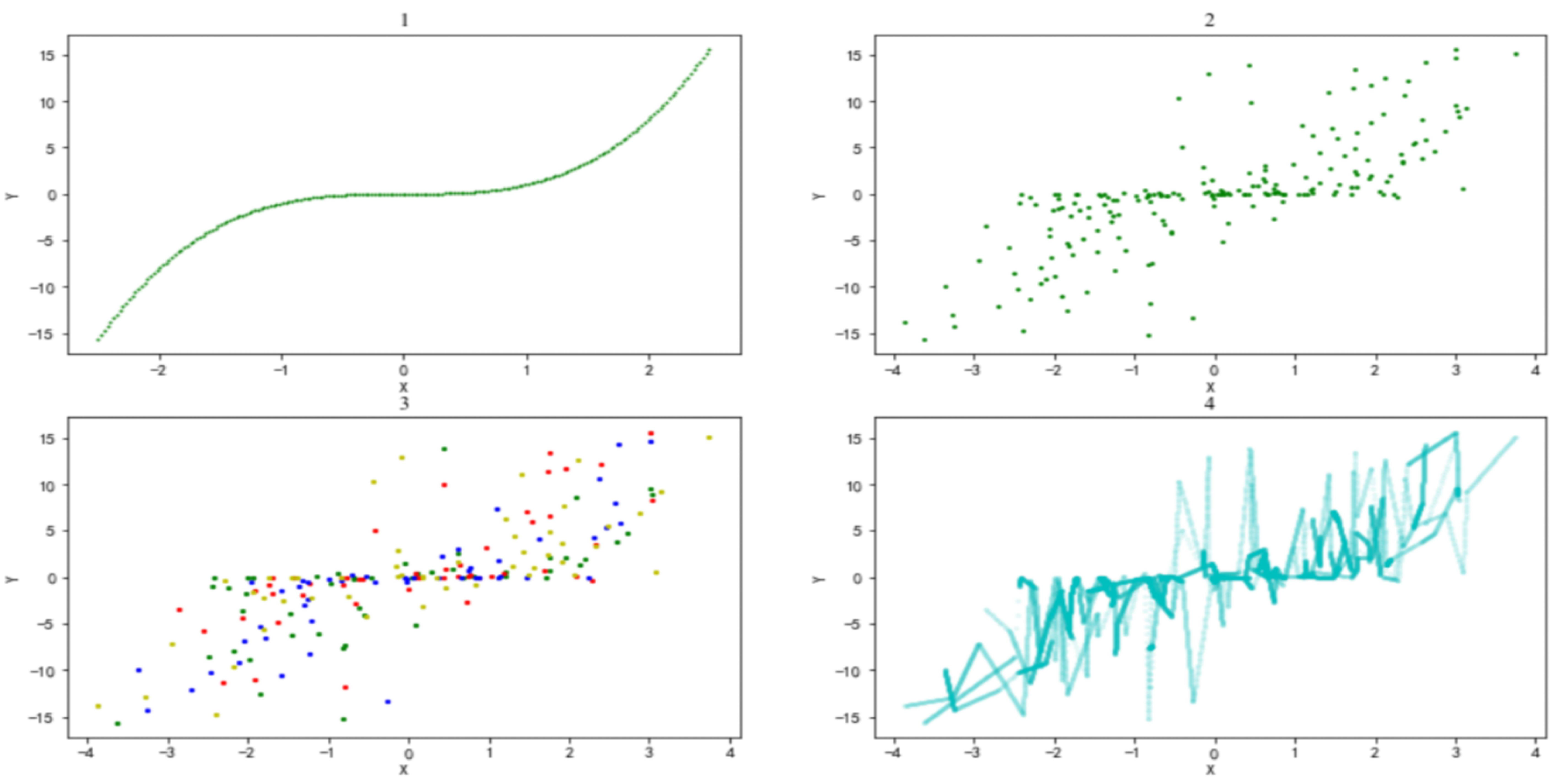
To reflect the optimization effect of the AMLI method more visually, below, we describe the AMLI processing process of simulation 1 in detail. First, 200 samples are generated evenly in the interval of (−2.5, 2.5) (Figure 1(1)). Second, noise that obeys the standard normal distribution is added to the feature variables (Figure 1(2)). Third, to achieve a better visualization effect, original samples are divided into only four categories (just to achieve a better visualization effect, and the verification index is not necessarily optimal) (i.e., the hyperparameter K = 4) with labels of different colors (Figure 1(3)). Fourth, given the small interval of the definition domain, high values of the unit distance filling parameter are selected, and sample filling is performed after setting the hyperparameter η = 100. After the filling, the sample size reaches 3035 (Figure 1(4)).
The comparison of the visualization effects in Figure 1(2) and Figure 1(4) indicates that after processing with the AMLI method, the samples can adaptively fit the functional relationship between x and y.
By using the above method, the parameters of the six simulations are calibrated, and the verification indicators are calculated, as shown in Table 1.
Remark 1.
The optimal effect of each simulation is determined by the lowest M S E after AMLI processing by traversing all the hyperparameter values according to the grid search method.
Clearly, after the AMLI processing, the M S E of the samples and the proportion of various error samples have been optimized, most of the added dummy samples are valid ones, the increase in the sample size does not significantly weaken the AMLI’s optimization effect, the samples that obey the normal distribution have better optimization performance, and even the uniformly distributed noise shows good robustness. In many cases, the AMLI method performs well in data optimization.

3.2. Analysis of Hyperparameter Taking Values

In this section, we discuss the patterns of setting the parameters of K and η in the AMLI method. First, we examine the setting of parameter 
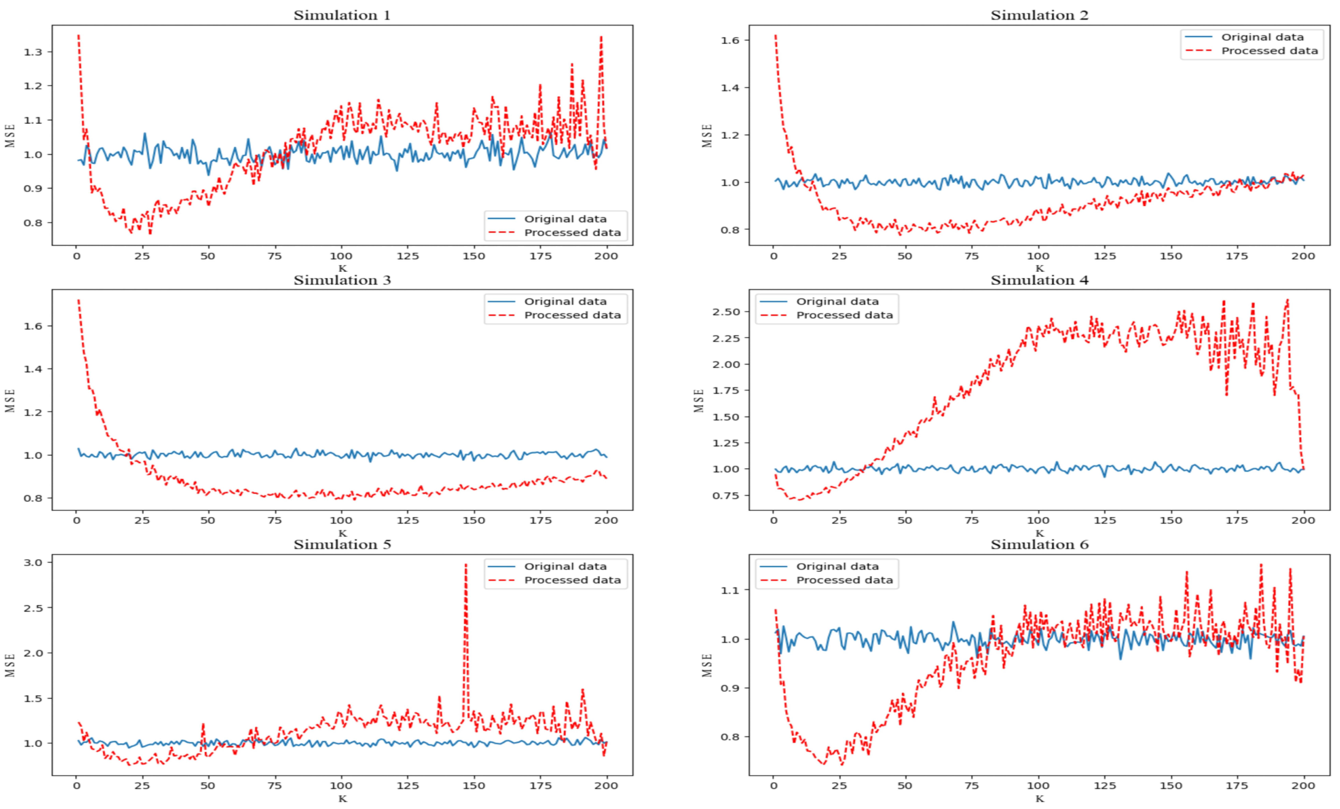
K. For the above simulation, we set the parameter η = 100; perform traversal iterations consecutively by setting K = 1 , 2 , 200 ; and obtain the average value of the index for one hundred iterations at each setting. The change trend of the MSE index before and after the AMLI processing is shown in Figure 2.
At fixed parameter η values, the optimal value of K increases with the increase in the sample size; the value range of K varies under different distributions of variables; and the change in the noise distribution has little impact on the optimal value of K.
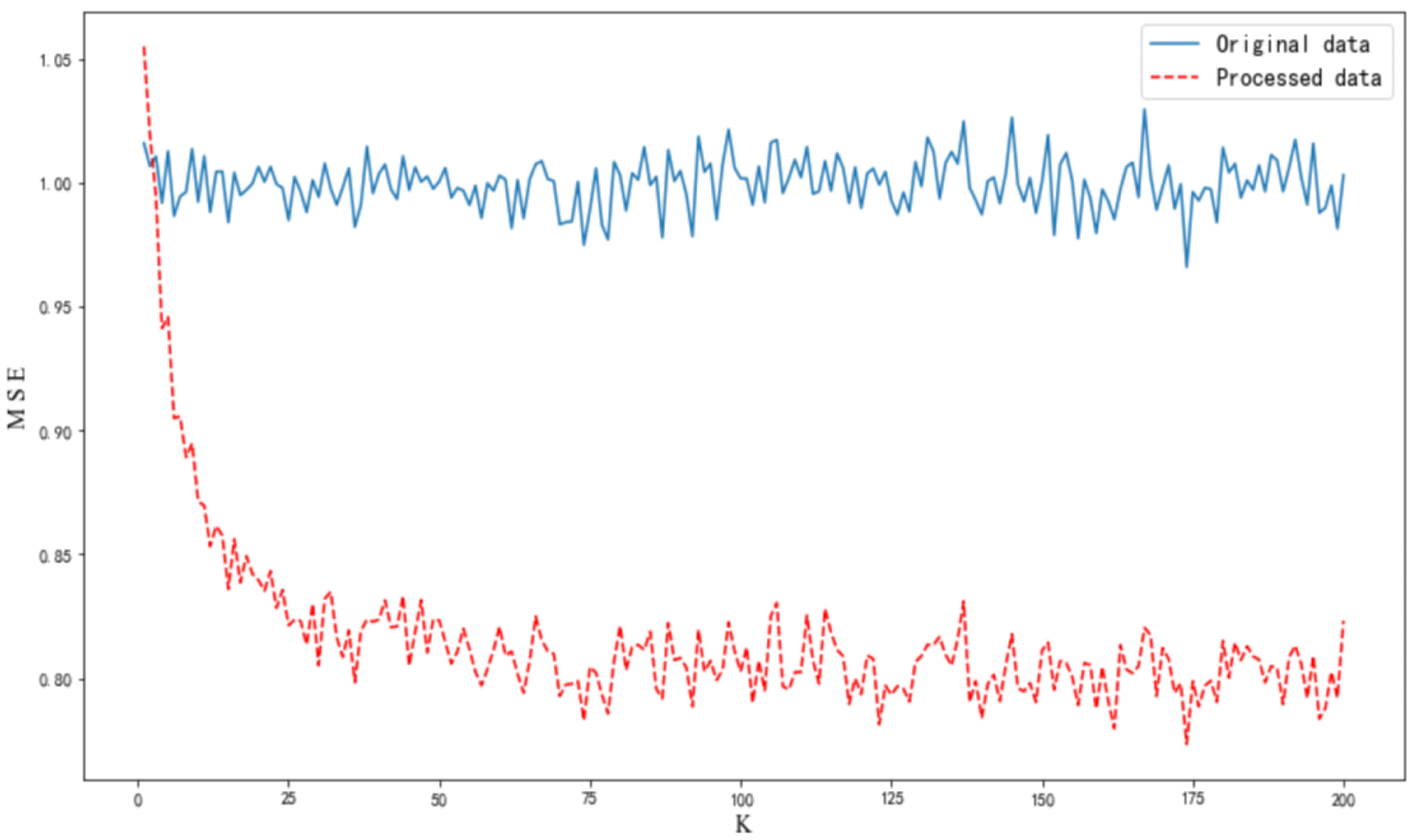
Next, we examine the pattern of the setting of parameter η . In the case of simulation 1, under the condition of K = 21 to take the optimal value, traversal iterations are performed consecutively by setting the parameter η = 1 , 2 , , 200 ; the results are shown in Figure 3. Clearly, the fluctuation of the sample M S E after optimization by using the AMLI method decreases with the increase in the value of filling parameter η .

3.3. Comparison with Other Interpolation Methods

The above experiments show that the AMLI method can greatly expand valid samples and reduce the uniform error of samples as a whole so that the proportion of samples with large errors is low. The AMLI method achieves sample optimization based mainly on the idea of interpolation. The main interpolation methods include linear interpolation, quadratic spline interpolation and cubic spline interpolation. In this section, we will compare the AMLI method with other interpolation methods to demonstrate its superiority.
Similarly, simulation 1 is used as the control group, and simulations 2–6 are used as the experimental group, using various interpolation methods with a fixed interpolation number of 3500–4000. Only the MSE between the processed samples and the actual values is selected as the evaluation index, and for each simulation, one hundred experiments are carried out, and their average value is taken. The results are shown in Table 2. In terms of the M S E , the A M L I method clearly outperforms the other methods, indicating that the A M L I method has achieved a very significant optimization effect.

4. Application of AMLI Method in Machine Learning

In this section, we will describe the performance of the AMLI method in both simulated and actual data prediction when the method is combined with various machine learning models. Using the side-by-side method, we divide the training set and the test set in the ratio of 7:3; the training set is optimized by using the AMLI method. For the machine learning method, we select the K-Nearest Neighbor ( K N N ) method, Feedforward Neural Network ( F N N ), Gradient Boosting Decision Tree ( G B D T ) and Random Forest ( R F ), with the M S E as the loss function. The hyperparameters of each model and the parameters of K and η of the AMLI method are calibrated multiple times to obtain the optimal values. The Euclidean distance is adopted as the distance function:
M S E = 1 N i = 1 N ( y i y ^ i ) 2 ,
L ( x i , x j ) = l = 1 n ( x i l x j l ) 2 .

4.1. Simulated Data Prediction

We assume that for simulated samples with a size of 1000, the simulated data feature dimension n = 3 , different feature dimensions obey different distributions, x 1 N ( 0 , 3 ) , x 2 U ( 3 , 3 ) , x 3 t ( 5 ) , and the weight vector of w ( 3 , 2 ) 1 , w ( 2 , 1 ) 2 is randomly generated. Let Y = X · w ( 3 , 2 ) 1 · w ( 2 , 1 ) 2 + ϵ ˜ . After the data are generated, noise that obeys the Gaussian distribution is added to X , which is then further divided into the test set and the training set. The training set is processed using the A M L I method (K = 40, η = 5), and the total number of samples after the processing is 9810.
As shown in Table 3, the M S E of the trained model using the data processed by the A M L I method is smaller in the prediction, indicating that the prediction result is more accurate.

4.2. Actual Data Prediction

4.2.1. Demand Forecast for Shared Bike Rental

In this section, we present a case study by predicting the demand for shared bicycle rentals in a certain city. The dataset includes multiple variables, such as season, holiday, temp, and registered (Table 4). We use the AMLI method to optimize samples of actual data. On the one hand, we combine the AMLI method with machine learning methods to examine its optimization performance in actual predictions; on the other hand, given that the dataset contains multiple categorical data, we can explore whether the AMLI method can achieve good optimization in prediction when the assumptions of the AMLI method are violated.
The dataset contains 7620 observation samples. We select 1000, 3000, and 7620 samples consecutively to examine the prediction optimization of the AMLI method in combination with machine learning methods when the sample size is insufficient, fair, or sufficient.
As shown in Table 5, at various sample size levels, the AMLI method has achieved a certain optimization of prediction effect.

4.2.2. Concentration Forecast for P M 2.5

In this section, we present a case study by predicting the concentration for P M 2.5 in a certain city to rule out the randomness of the dataset. The dataset includes multiple concentrations of air pollutants such as P M 10 , CO, S O 2 , N O 2 and O 3 . The dataset contains 3193 observation samples. We select 500, 1500, and 3193 samples consecutively to examine the prediction optimization of the A M L I method. As shown in Table 6, the A M L I method still has a good optimization effect.

5. Proof

In this section, we will present the proof for the samples that satisfy the AMLI hypothesis that after processing with the AMLI method, the average observation error of the samples is reduced, and the proportion of samples with different errors is adjusted.
The rationale of AMLI is to divide the original feature space into N / K subspaces with K samples, randomly extract a sample from each subspace as a class to divide the original dataset into K classes, and then perform linear interpolation between two adjacent samples. In essence, AMLI can be viewed as a method of linear interpolation between two subspaces with close distances through K paths.
For the dataset T = { ( x 1 , y 1 ) , ( x 2 , y 2 ) , , ( x N , y N ) } , we select two subspaces that are assumed to have equal samples: X ( 1 ) , X ( 2 ) X R , and X ( 1 ) X ( 2 ) = . In these two subspaces, we assume the following common relation is present:
y = f ( x * ) + ϵ ˜ = f ( x ϵ ) + ϵ ˜ ,
where x * is the actual value of x after removing the observation noise; and where x = x * + ϵ , where ϵ is the noise term, ϵ N ( 0 , σ 2 ) , and ϵ ˜ i is the model error.
According to our assumption, f ( · ) is a continuous function; if X ( 1 ) , X ( 2 ) 0 , and X ( 1 ) X ( 2 ) = , d i s ( X ( 1 ) , X ( 2 ) ) 0 , f ( · ) can be approximated as a linear function of g ( · ) , and then (1) can be transformed into
y = g ( x * ) + ϵ 1 + ϵ ˜ = g ( x ϵ ) + ϵ 1 + ϵ ˜ ,
where ϵ 1 is the linear fitting error term and ϵ 1 0 .
Since the samples we select in X ( 1 ) , X ( 2 ) are equal in size, we assume there are K observation samples; i.e., x ( j ) = ( x 1 ( j ) , , x K ( j ) ) = ( x 1 * ( j ) + ϵ 1 ( j ) , , x K * ( j ) + ϵ K ( j ) ) X ( j ) , j = 1 , 2 . The expectation of the absolute value of the uniform noise in the space at this time is X ( 1 ) , X ( 2 ) :
E ( j = 1 2 i = 1 K | ϵ i ( j ) | 2 K ) = + | t | 1 2 π · σ e t 2 2 σ 2 d t = 2 π · σ 0 + t σ t t 2 2 σ 2 d t σ = 2 π · σ 0 + e t 2 2 σ 2 d ( t σ ) 2 2 = 2 π · σ · Γ ( 1 ) = 2 π · σ .
The expectation of the proportion of observed samples with a noise greater than 0.5 is
E ( j = 1 2 i = 1 K I ( | x i ( j ) x i * ( j ) | ) > 0.5 2 K ) = E ( j = 1 2 i = 1 K I ( | ϵ i ( j ) | ) > 0.5 2 K ) = j = 1 2 i = 1 K ( P ( ϵ i ( j ) > 0.5 ) + P ( ϵ i ( j ) < 0.5 ) ) 2 K = j = 1 2 i = 1 K ( P ( ϵ i ( j ) σ > 0.5 σ ) + P ( ϵ i ( j ) σ < 0.5 σ ) ) 2 K = j = 1 2 i = 1 K Φ ( 0.5 σ ) K = 2 Φ ( 0.5 σ ) .
We randomly select two samples from the subspace to perform linear interpolation on them and iterate the process K times. The AMLI method determines the number of interpolation samples according to the distance between two samples. For the sake of simplicity and convenience, we assume that the number of samples in each interpolation is m, and the rest of the situation is similar and provable. The sample for the ith interpolation is
x i = ( x i , 1 , x i , 2 , , x i , m ) = ( x i ( 1 ) + x i ( 2 ) x i ( 1 ) m + 1 , x i ( 1 ) + 2 · x i ( 2 ) x i ( 1 ) m + 1 , , x i ( 1 ) + m · x i ( 2 ) x i ( 1 ) m + 1 ) = ( x i * ( 1 ) + ϵ i ( 1 ) + x i * ( 2 ) x i * ( 1 ) + ϵ i ( 2 ) ϵ i ( 1 ) m + 1 , , x i * ( 1 ) + ϵ i ( 1 ) + m · x i * ( 2 ) x i * ( 1 ) + ϵ i ( 2 ) ϵ i ( 1 ) m + 1 ) ,
where i = 1 , , K and the corresponding output is y i , d = y i ( 1 ) + d · y i ( 2 ) y i ( 1 ) m + 1 . Based on (2), the noise of x i , d is ϵ i , d = ϵ i ( 1 ) + d · ϵ i ( 2 ) ϵ i ( 1 ) m + 1 , d = 1 , , m .
After K interpolations, the uniform noise expectation is
E ( j = 1 2 i = 1 K | ϵ i ( j ) | + i = 1 K d = 1 m | ϵ i ( 1 ) + d · ϵ i ( 2 ) ϵ i ( 1 ) m + 1 | 2 K + K · m ) = j = 1 2 i = 1 k E ( | ϵ i ( j ) | ) + i = 1 K d = 1 m E ( | ϵ i ( 1 ) + d · ϵ i ( 2 ) ϵ i ( 1 ) m + 1 | ) 2 K + K · m = j = 1 2 i = 1 K E ( | ϵ i ( j ) | ) + 1 m + 1 i = 1 K d = 1 m E ( | ( m d + 1 ) ϵ i ( 1 ) + d ϵ i ( 2 ) | ) 2 K + K · m = 2 + 1 m + 1 d = 1 m ( m d + 1 ) 2 + d 2 2 + m · σ 2 π < 2 + 1 m + 1 d = 1 m ( m d + 1 ) 2 + d 2 + 2 d ( m d + 1 ) 2 + m · σ 2 π = 2 + 1 m + 1 d = 1 m ( m + 1 ) 2 2 + m · σ 2 π = σ 2 π .
The above shows that the uniform noise of the samples after the optimization through the AMLI method is reduced. The expectation for the proportion of samples with a noise greater than 0.5 is
E ( j = 1 2 i = 1 K I ( | ϵ i ( j ) | > 0.5 ) + i = 1 K d = 1 m I ( | ϵ i ( 1 ) + d · ϵ i ( 2 ) ϵ i ( 1 ) m + 1 | > 0.5 ) 2 K + K · m ) = 4 K · Φ ( 0.5 σ ) + i = 1 K d = 1 m p ( | ϵ i ( 1 ) + d · ϵ i ( 2 ) ϵ i ( 1 ) m + 1 | > 0.5 ) 2 K + K · m = 4 K · Φ ( 0.5 σ ) + i = 1 K d = 1 m p ( | ( m d + 1 ) ϵ i ( 1 ) + d · ϵ i ( 2 ) | ( m d + 1 ) 2 + d 2 · σ > 0.5 ( m + 1 ) ( m d + 1 ) 2 + d 2 · σ ) 2 K + K · m = 4 Φ ( 0.5 σ ) + 2 d = 1 m Φ ( 0.5 ( m + 1 ) ( m d + 1 ) 2 + d 2 · σ ) 2 + m < 4 Φ ( 0.5 σ ) + 2 d = 1 m Φ ( 0.5 ( m + 1 ) ( m d + 1 ) 2 + d 2 + 2 d ( m d + 1 ) · σ ) 2 + m = 2 Φ ( 0.5 σ ) .
Thus, after being processed by the AMLI method, the proportion of samples with an error greater than 0.5 in the data decreases.

6. Extension

6.1. AMLI Plus

The above simulation experiments indicate that the selection of parameter K in the AMLI algorithm is very important. The selection of the optimal value of parameter K involves many parameter adjustment calculations while under the influence of randomness, thereby making it difficult to guarantee that the selected K value results in optimal performance at all times. If the AMLI method fails to achieve a good result, we can consider another interpolation method that combines the clustering method to perform linear interpolation between classes; we name this method AMLI plus. Below, we describe specific steps of the AMLI plus method.
First, all observed samples are clustered according to their distribution. Assuming that the number of clusters is K, and accordingly, the virtual space is divided into K subspaces, each containing all observed samples of the same category:
T = { ( x 1 , y 1 ) , ( x 2 , y 2 ) , , ( x k , y k ) } = { G 1 , G 2 , , G K } ,
where G 1 represents the class whose center is closest to the minimum point of the feature space x 0 ; the center of the class is x ¯ ( d ) = 1 n ( d ) i = 1 n ( d ) x i ( d ) , d = 1 , , K , n ( d ) G d , d = 1 , , K ; n ( d ) is the number of samples in G d ; and G d + 1 satisfies x ¯ ( d + 1 ) = a r g m i n { x ¯ : x ¯ x ¯ ( 1 ) , , x ¯ ( d ) } ( L ( x ¯ ( d ) , x ¯ ) ) . The choice of clustering method can be diverse; additionally, the K- m e a n s , the X- m e a n s or the D B S C A N method, which can eliminate noise points according to Ester et al. [15], can be selected.
Second, interpolation is performed between classes, in which the unit distance filling parameter η is defined; additionally, n ( d ) · n ( d + 1 ) linear interpolations are performed between x i ( d ) G d and all samples in G d + 1 . The number of interpolation samples is j = 1 n ( d + 1 ) i = 1 n ( d ) η · L ( x i ( d ) , x j ( d + 1 ) ) , and the interpolated samples are also equally spaced.
The specific implementation process of the AMLI method is detailed in Algorithm 2.   
Algorithm 2: AMLI plus
Mathematics 11 00768 i002

6.2. The Proof of AMLI Plus

In this section, we will present evidence of the effectiveness of the AMLI plus method. The proof idea is essentially the same as that of the AMLI method, and we will focus on the differences between the two.
Unlike the AMLI method, the AMLI plus method divides the virtual space into K subspaces according to the number of clusters, and each subspace contains all observation samples of the same category; thus, the sample size of each subspace may vary. It is assumed that two adjacent subspaces, namely, X ( 1 ) , X ( 2 ) , contain n ( 1 ) , n ( 2 ) samples, respectively; additionally, it is assumed that n ( 1 ) · n ( 2 ) linear interpolations are performed. For the sake of simplicity, assuming that the number of samples interpolated each time is m, then the uniform noise after the interpolation is
E ( i = 1 n ( 1 ) | ϵ i ( 1 ) | + i = 1 n ( 2 ) | ϵ i ( 2 ) | + i = 1 n ( 1 ) j = 1 n ( 2 ) d = 1 m ϵ i ( 1 ) + d · ϵ j ( 2 ) ϵ i ( 1 ) m + 1 n ( 1 ) + n ( 2 ) + n ( 1 ) n ( 2 ) m ) = i = 1 n ( 1 ) E ( | ϵ i ( 1 ) | ) + i = 1 n ( 2 ) E ( | ϵ i ( 2 ) | ) + i = 1 n ( 1 ) j = 1 n ( 2 ) d = 1 m E ( ϵ i ( 1 ) + d · ϵ j ( 2 ) ϵ i ( 1 ) m + 1 ) n ( 1 ) + n ( 2 ) + n ( 1 ) n ( 2 ) m = n ( 1 ) σ 2 n + n ( 2 ) σ 2 n + 1 m + 1 i = 1 n ( 1 ) j = 1 n ( 2 ) d = 1 m E ( ( m d + 1 ) ϵ i ( 1 ) + d ϵ i ( 2 ) ) n ( 1 ) + n ( 2 ) + n ( 1 ) n ( 2 ) m = n ( 1 ) + n ( 2 ) + n ( 1 ) n ( 2 ) m + 1 d = 1 m ( m d + 1 ) 2 + d 2 n ( 1 ) + n ( 2 ) + n ( 1 ) n ( 2 ) m · σ 2 π < n ( 1 ) + n ( 2 ) + n ( 1 ) n ( 2 ) m + 1 d = 1 m ( m d + 1 ) 2 + d 2 + 2 d ( m d + 1 ) n ( 1 ) + n ( 2 ) + n ( 1 ) n ( 2 ) m · σ 2 π = n ( 1 ) + n ( 2 ) + n ( 1 ) n ( 2 ) m + 1 d = 1 m m + 1 n ( 1 ) + n ( 2 ) + n ( 1 ) n ( 2 ) m · σ 2 π = σ 2 π .
Thus, the uniform noise after optimization by the AMLI plus method is reduced. The proportion of samples with a noise error greater than 0.5 is expected to be
E ( i = 1 n ( 1 ) I ( | ϵ i ( 1 ) | > 0.5 ) + i = 1 n ( 2 ) I ( | ϵ i ( 2 ) | > 0.5 ) + i = 1 n ( 1 ) j = 1 n ( 2 ) d = 1 m I ( ϵ i ( 1 ) + d · ϵ j ( 2 ) ϵ i ( 1 ) m + 1 > 0.5 ) n ( 1 ) + n ( 2 ) + n ( 1 ) n ( 2 ) m ) = i = 1 n ( 1 ) P ( | ϵ i ( 1 ) | > 0.5 ) + i = 1 n ( 2 ) P ( | ϵ i ( 2 ) | > 0.5 ) + i = 1 n ( 1 ) j = 1 n ( 2 ) d = 1 m P ( ϵ i ( 1 ) + d · ϵ j ( 2 ) ϵ i ( 1 ) m + 1 > 0.5 ) n ( 1 ) + n ( 2 ) + n ( 1 ) n ( 2 ) m = 2 ( n ( 1 ) + n ( 2 ) ) Φ 0.5 σ + i = 1 n ( 1 ) j = 1 n ( 2 ) d = 1 m P ( | ( m d + 1 ) ϵ i ( 1 ) + d · ϵ j ( 2 ) | ( m d + 1 ) 2 + d 2 · σ > 0.5 ( m + 1 ) ( m d + 1 ) 2 + d 2 · σ ) n ( 1 ) + n ( 2 ) + n ( 1 ) n ( 2 ) m = 2 ( n ( 1 ) + n ( 2 ) ) Φ 0.5 σ + 2 n ( 1 ) n ( 2 ) d = 1 m Φ 0.5 ( m + 1 ) ( m d + 1 ) 2 + d 2 · σ n ( 1 ) + n ( 2 ) + n ( 1 ) n ( 2 ) m < 2 ( n ( 1 ) + n ( 2 ) ) Φ 0.5 σ + 2 n ( 1 ) n ( 2 ) d = 1 m Φ 0.5 ( m + 1 ) ( m d + 1 ) 2 + d 2 + 2 d ( m d + 1 ) · σ n ( 1 ) + n ( 2 ) + n ( 1 ) n ( 2 ) m = 2 Φ 0.5 σ .
Therefore, after the samples are processed by the AMLI plus method, the proportion of samples with an error greater than 0.5 in the data decreases.
Remark 2.
The proof rationale of the AMLI plus method is to divide the clustered samples of different categories into different subspaces and to assume that neighboring subspaces have a common linear relationship; therefore, when the number of clusters and the clustering method are selected, the above requirement should be satisfied as much as possible.

7. Conclusions

In this study, we propose a multipath sample interpolation method based on the idea of linear interpolation, which can solve the problem of insufficient sample sizes or large errors between observed samples and actual distribution when making predictions. The AMLI method, simple to implement and flexible, can greatly expand valid samples, reduce the influence of sample noise, and thus significantly improve the prediction effect. Finally, we propose the AMLI plus method, another class-to-class-based linear interpolation method, which can also achieve good optimization results. In general, we find that the AMLI method is robust, effective, and very suitable for addressing a series of problems in machine learning, e.g., insufficient sample sizes and large amounts of observation noise.

Author Contributions

Methodology, H.W.; Software, Y.D.; Writing—original draft, X.J.; Writing—review & editing, M.L. All authors have read and agreed to the published version of the manuscript.

Funding

This research was supported by the National Social Science Fund of China under Grant No. 22BTJ021, “Qinglan project” of Colleges and Universities of Jiangsu Province and Postgraduate Research & Practice Innovation Program of Jiangsu Province under Grant No. KYCX22_2148.

Institutional Review Board Statement

Not applicable.

Informed Consent Statement

Not applicable.

Data Availability Statement

Not applicable.

Acknowledgments

The authors would like to thank the editor and reviewers for the valuable advice given in order to develop the article.

Conflicts of Interest

The authors declare no conflict of interest.

References

  1. De Boor, C. A Practical Guide to Splines; Springer: New York, NY, USA, 1978. [Google Scholar]
  2. Mitas, L.; Mitasova, H. Spatial interpolation. Geogr. Inf. Syst. Princ. Tech. Manag. Appl. 1999, 1, 481–492. [Google Scholar]
  3. Lu, G.Y.; Wong, D.W. An adaptive inverse distance weighting spatial interpolation technique. Comput. Geosci. 2008, 34, 1044–1055. [Google Scholar] [CrossRef]
  4. Efron, B. Bootstrap methods: Another look at the jackknife. In Breakthroughs in Statistics; Springer: New York, NY, USA, 1992; pp. 569–593. [Google Scholar]
  5. Chawla, N.V.; Bowyer, K.W.; Hall, L.O.; Kegelmeyer, W.P. SMOTE: Synthetic minority over-sampling technique. J. Artif. Intell. Res. 2002, 16, 321–357. [Google Scholar] [CrossRef]
  6. Pan, S.J.; Yang, Q. A survey on transfer learning. IEEE Trans. Knowl. Data Eng. 2010, 22, 1345–1359. [Google Scholar] [CrossRef]
  7. Fernández, A.; Garcia, S.; Herrera, F.; Chawla, N.V. SMOTE for learning from imbalanced data: Progress and challenges, marking the 15-year anniversary. J. Artif. Intell. Res. 2018, 61, 863–905. [Google Scholar] [CrossRef]
  8. Zhu, X.J. Semi-Supervised Learning Literature Survey; University of Wisconsin-Madison: Madison, WI, USA, 2005. [Google Scholar]
  9. Eisenberger, M.; Novotny, D.; Kerchenbaum, G.; Labatut, P.; Neverova, N.; Cremers, D.; Vedaldi, A. Neuromorph: Unsupervised shape interpolation and correspondence in one go. In Proceedings of the IEEE/CVF Conference on Computer Vision and Pattern Recognition, Nashville, TN, USA, 20–25 June 2021; pp. 7473–7483. [Google Scholar]
  10. Wang, Y.; Yao, Q.; Kwok, J.T.; Ni, L.M. Generalizing from a few examples: A survey on few-shot learning. ACM Comput. Surv. 2020, 53, 1–34. [Google Scholar] [CrossRef]
  11. Vinyals, O.; Blundell, C.; Lillicrap, T.; Wierstra, D. Matching networks for one shot learning. Adv. Neural Inf. Process. Syst. 2016, 29, 3637–3645. [Google Scholar]
  12. Snell, J.; Swersky, K.; Zemel, R. Prototypical networks for few-shot learning. Adv. Neural Inf. Process. Syst. 2017, 30, 4077–4087. [Google Scholar]
  13. Kokol, P.; Kokol, M.; Zagoranski, S. Machine learning on small size samples: A synthetic knowledge synthesis. Sci. Prog. 2022, 105, 1–15. [Google Scholar] [CrossRef] [PubMed]
  14. Zhou, Y.; Zhi, G.; Chen, W.; Qian, Q.; He, D.; Sun, B.; Sun, W. A new tool wear condition monitoring method based on deep learning under small samples. Measurement 2022, 189, 110622. [Google Scholar] [CrossRef]
  15. Ester, M.; Kriegel, H.P.; Sander, J.; Xu, X. A density-based algorithm for discovering clusters in large spatial databases with noise.kdd. KDD 1996, 96, 226–231. [Google Scholar]
Figure 1. Steps of AMLI processing.
Mathematics 11 00768 g001
Figure 2. Changes in the M S E under different K values.
Mathematics 11 00768 g002
Figure 3. Changes in the M S E under different η values.
Mathematics 11 00768 g003
Table 1. Monte Carlo simulation results.
SimulationMSE p ( 0.5 ) p ( 1 ) p ( 1.5 ) p ( 2 ) p ( 2.5 )
BeforeAfterBeforeAfterBeforeAfterBeforeAfterBeforeAfterBeforeAfter
10.9570.7620.6040.5700.3160.2510.1300.0830.0360.0220.0100.006
20.9800.7740.6140.5670.3130.2580.1320.0890.0430.0230.0110.005
30.9770.7890.6190.5710.3080.2540.1310.0900.0430.0250.0110.005
40.9900.7010.6090.5490.3170.2320.1330.0730.0440.0170.0110.003
50.9820.7560.6110.5520.3060.2450.1270.0850.0380.0240.0100.005
60.9870.7420.7060.6320.4110.2970.1260.0570.0000.0000.0000.000
Table 2. M S E values of samples under different interpolation methods.
SimulationMSE
AMLILinear InterpolationQuadratic SplineCubic Spline
10.7621.3855.5429.452
20.7741.6186.4348.976
30.7891.8126.4418.338
40.7011.57818.15642.997
50.7561.20310.32229.542
60.7420.9594.8026.619
Table 3. Simulation data prediction results.
MSEKNNFNNGBDTRF
Before AMLI processing1.700.9421.2101.507
After AMLI processing1.070.7131.0081.320
Table 4. Description of variable indicators.
Variable NameVariable Definition
Season1 = Spring
2 = Summer
3 = Autumn
4 = Winter
Holiday1 = Holiday
0 = Non-holiday
Workdays1 = Working day
0 = Weekend
Weather1 = Sunny, cloudy
2 = Foggy, overcast
3 = Light snow, drizzle
4 = Heavy rain, heavy snow, heavy fog
TempTemperature in Celsius
AtempApparent temperature
HumidityHumidity
WindspeedWind speed
CasualNumber of nonregistered users
RegisteredNumber of registered users
CountTotal number of car rentals
Table 5. Prediction results of shared bicycle rental demand (MSE).
NHyper-ParameterN (After Processing)AMLI ProcessingKNNFNNGBDTRF
1000 K = 25 191,057Before208.2300.967788.152231.210
η = 5 After46.3400.079168.394158.940
3000 K = 40 290,856Before42.7570.334222.79443.679
η = 3 After26.0200.008414.30125.451
7620 K = 65 428,277Before17.4640.11689.87923.521
η = 1 After6.7980.00516.9812.472
Table 6. Prediction results of shared bicycle rental demand ( M S E ( 10 3 ) ) .
NHyperparameterN (After Processing)AMLI Processing KNN FNN GBDT RF
500 K = 17 1089Before3.164.453.143.39
η = 10 After2.892.552.363.01
1500 K = 23 7003Before2.692.542.332.62
η = 30 After2.182.071.862.33
3193 K = 50 24,559Before1.771.631.481.54
η = 60 After1.411.131.071.16
Disclaimer/Publisher’s Note: The statements, opinions and data contained in all publications are solely those of the individual author(s) and contributor(s) and not of MDPI and/or the editor(s). MDPI and/or the editor(s) disclaim responsibility for any injury to people or property resulting from any ideas, methods, instructions or products referred to in the content.

