1. Introduction
In the field of mineral resource estimation, it is common practice to identify volumes that are spatially consistent, statistically similar, and geologically distinct from other volumes around them. These are called estimation domains in the geostatistical literature [
1], and entail an improvement in the performance of estimation techniques. The geological aspects of the deposit are usually the fundamental guidelines for the definition of estimation domains. Attributes such as alteration, mineralization, and lithological aspects must be considered [
2]. Glacken and Snowden [
3] state that a geological domain represents an area or volume within which the characteristics of mineralization are more similar than outside the domain. Other authors [
1] are more specific and define geological domains as the equivalent of geostatistically stationary zones.
In mineral resource modeling, the concept of stationarity is closely related to the homogeneity of geological bodies, and simplifying the definition that authors give in [
4], it can be assumed that a phenomenon is stationary when it shows constant expected values, covariance, and self-correlation structures at any given location in the studied area. Estimation domains that do not adhere to the stationarity principle can lead to significant bias in mineral grades and, therefore, erroneous estimates [
5]. In this article, the concept of geostatistical domain is directly associated with the geological domain of estimation. Thus, there will be no distinction in the term and in a simplified way, we will speak of estimation domains.
The traditional methodology used to define estimation domains for mineral resources is based on a combined study between geology and statistics, in which geological understanding and human intervention predominate. At a general level, the steps that this methodology follows are:
Selection of geological attributes that control mineral grade.
Statistical analysis of the mineral grade for each category of each geological attribute.
Combination of categories of each geological attribute by statistical similarity and spatial soft contact. The latter is also known as the definition of geological units (alteration, lithology, mineralization, etc.).
Combination of geological attributes (units) by statistical similarity and spatial soft contact.
Validation of the estimation domains at the geological, statistical, and geostatistical level.
Nevertheless, this methodology has some critical aspects. One of them is that it is slow, since all the works must be carried out and checked by an acquaintance in the geology of the mineral deposit. It is also subjective, since, from one expert to another, different criteria and interpretations are manifested. Codes for reporting mineral resources are intended to define minimum standards [
6], and this opens the possibility of using multiple methods as long as they can be supported. Further, the behavior of the mineral grade will not necessarily be homogeneous; it will present stationarity and its spatial structure could be interpreted in different ways. This occurs because domains depend closely on geological attributes that will not necessarily be grouped by the characteristics mentioned above.
In this study, the implementation of a methodology based on unsupervised machine learning is evaluated, through the use of a multivariate clustering algorithm. The main objectives are to obtain a new alternative to define estimation domains that satisfies the principles of geostatistical estimation, to reduce the time factor that is criticized for the traditional methodology and to decrease the subjectivity of the traditional methods.
Clustering algorithms have been used since the 1960s, when Sokal et al. [
7] introduced the hierarchical agglomerative technique to work in the field of taxonomy, and MacQueen [
8] introduced the k-means algorithm. This approach may be especially appropriate for the definition of estimation domains, since it divides the data into groups based on the relationships between the more relevant variables of the problem [
9]. Automatic grouping is an approach to analyze spatial data at a higher level of abstraction by grouping according to their similarity into significant groups [
10]. A collection of data is organized into groups so that items within a group are more “similar” to each other than to data in the other groups. Grouping is generally performed when no information is available about the membership of data items in predefined classes. For this reason, it is traditionally considered part of unsupervised learning [
11]. There are a wide variety of clustering approaches for different applications and data sizes [
12]. Some of these methods include hierarchical clustering, partition clustering, mixture model clustering, neural network-based clustering, fuzzy clustering, and graph clustering [
12,
13,
14].
One of the most popular and widespread algorithms in automatic grouping is k-means, which corresponds to a numeric, unsupervised, non-deterministic iterative method, which is simple and very fast. Therefore, in many practical applications, the method has proven to be a very effective way that can produce good clustering results [
15]. Other authors [
16] used k-means clustering to identify geological domains in an iron ore deposit, based on laboratory analysis data (Fe, SiO
, Al
O
, P, TiO
, and LOI).
In [
17], the k-means method is used to define geo-metallurgical domains in an iron deposit in northeastern Iran, using data from laboratory analysis (Fe, FeO, S), magnetic susceptibility, and spatial coordinates (
X,
Y,
Z). Moreira et al. [
9] used k-means to define estimation geological domains in a phosphate–titanium deposit, mainly using data from laboratory analysis (P
O
, TiO
, and CaO), rock type, and alteration.
However, k-means optimizes a cost function defined on the Euclidean distance measure between data points and means. Minimizing the cost function by calculating means limits its use to numeric data [
18]. This limitation affects categorical geological variables that control the mineral grade, not being able to provide information on the grouping. Given this problem, the categorical data can be transformed to continuous, assuming an absolute knowledge of the associations of the categories of each geological attribute, which is complex. Another option consists in carrying out the inverse process. That is, to transform the continuous numeric variables of the mineral grades, to discrete ones, assuming a significant loss of information; then, a grouping algorithm for categorical data is used (such as k-modes [
18]). However, none of the options are suitable.
Few clustering methods have been proposed in the literature to deal with mixed data. Huang [
18] proposed the first algorithm that is based on a combinatorial of k-means and k-modes, which is known as k-prototypes. It makes possible to group mineral grades and geological attributes together. The algorithm groups objects with numeric and categorical attributes in a similar manner that k-means does. The object similarity measure is derived from both numeric and categorical attributes. When applied to numeric data, the algorithm is identical to k-means. Thus, an innovative fact of this manuscript is the practical application of this k-prototype clustering approach to the domain of geostatistical applications, as it has been usually applied to general big data cases.
When using unsupervised learning algorithms, the data are not labeled, so the correct answer is not known a priori. In this case, the non-hierarchical grouping algorithms need to be initialized indicating the number of groups as an input parameter. For the selection of the optimal number of groups, two different heuristics are used herein: the Calinski–Harabasz index [
19] and the Silhouette coefficient [
20].
The paper is organized as follows: in
Section 2, the methodology is explained; in
Section 3, the case study is analyzed; finally, in
Section 4, some conclusions are reported.
2. Methodology
The
k-prototypes algorithm allows the use of both numeric and categorical data. Given a data set of
n objects, where
are the numeric attributes and
the categorical, the goal of the
k-prototypes is to find
k clusters where the following objective function is minimized:
where
is an element of the partition matrix
, satisfying
and
.
P is a hard partition if
is a binary variable (
) that indicates the membership of the data
in cluster
l; otherwise,
P is a fuzzy partition.
is the center or prototype of cluster
l and
is the distance measure defined as follows:
represent the values of the numeric attributes and
the values of the categorical attributes for each data object
i;
is the mean of the
jth numeric attribute in a cluster
l, and
is the mode of the
jth categorical attribute in cluster
l;
is a weight for categorical attributes in a cluster
l. Function
, which is defined for categorical attributes, is:
The main algorithm of the
k-prototype method consists of calculating the distance between data objects and group centers or prototypes (
Q) using Equation (
2). The method finishes when the updated group center coincides with the group center of the previous iteration.
The
k-prototype method results adequate for small and medium data sets. However, it does not manage to treat mixed data sets on a large scale (millions of instances), due to the high computational cost that it requires (a total of
distance calculations in each iteration [
21]). The general workflow followed herein consisted in: we performed an exploratory data analysis (EDA), standardization of the data, application of the
k-prototype algorithm in 9 scenarios, selection of the optimal
k and validation of the estimation domains.
The purpose of the EDA is the description of the geological attributes that control the mineral grade, and the analysis of its behavior at a statistical and spatial level in each category of attributes. It is possible to deduce if the mineral grade is grouped in a single population or there are several independent populations. A requirement in automatic grouping is that each of the characteristics have the same influence. The latter is solved by data standardization. In this case, the
z-score is used:
where
z is the standardized value,
x the original value,
m the mean, and
s is the standard deviation of the original values. The result is a transformation, in which the same variance stands for all the characteristics.
Subsequently, the k-prototype algorithm is executed in 9 different scenarios being k in a range from 2 to 10. This is performed with the aim of selecting the optimal k, which is consistent with the number of clusters in which the inertia within the group is minimal and being groups distinguishable between them.
The first method used to select the optimal
k is the Calinski–Harabasz index (CH) [
19], which relates the internal metrics of cohesion and separation. Cohesion is understood as the closeness that the members must have within each group. It can be evaluated with the sum of the squares within each group (SSW):
where
k is the number of clusters,
x is a sample,
is the
ith cluster,
is the centroid of the cluster
, and
is the distance between
x and
.
On the other hand, the separation measures the dissimilarity that must exist between groups. It can be expressed by the sum of squares between groups (
SSB):
where
is the number of elements in cluster
ith,
is the centroid of cluster
ith and
is the mean of all the data points.
Finally, the
index is expressed as follows:
where
k is the number of clusters and
n the number of data points.
The process of selecting the optimal
k can be arbitrary when only one method is used. Therefore, a second method called the silhouette index (SH) [
20] is used. This method measures the separation distance between clusters, and it indicates how close each element of a cluster is to elements in neighboring clusters. This distance is on the interval
. A high positive value means good grouping. A value close to 0 indicates that the item is very close to or on the decision boundary between two clusters. Negative values indicate that the items may be assigned to the wrong group. The silhouette method calculates the mean of the silhouette coefficients of all the observations for different values of
k. The optimal number
k is the one that maximizes the mean of the silhouette coefficients for a range of
k values.
Given a point
, the coefficient of the silhouette is defined as:
where
is the mean distance between
and all the points in the cluster
, and
is the smallest distance between
and the sample from the nearest cluster that is not part of the cluster
.
The silhouette index of the whole grouping is given by the average of all
:
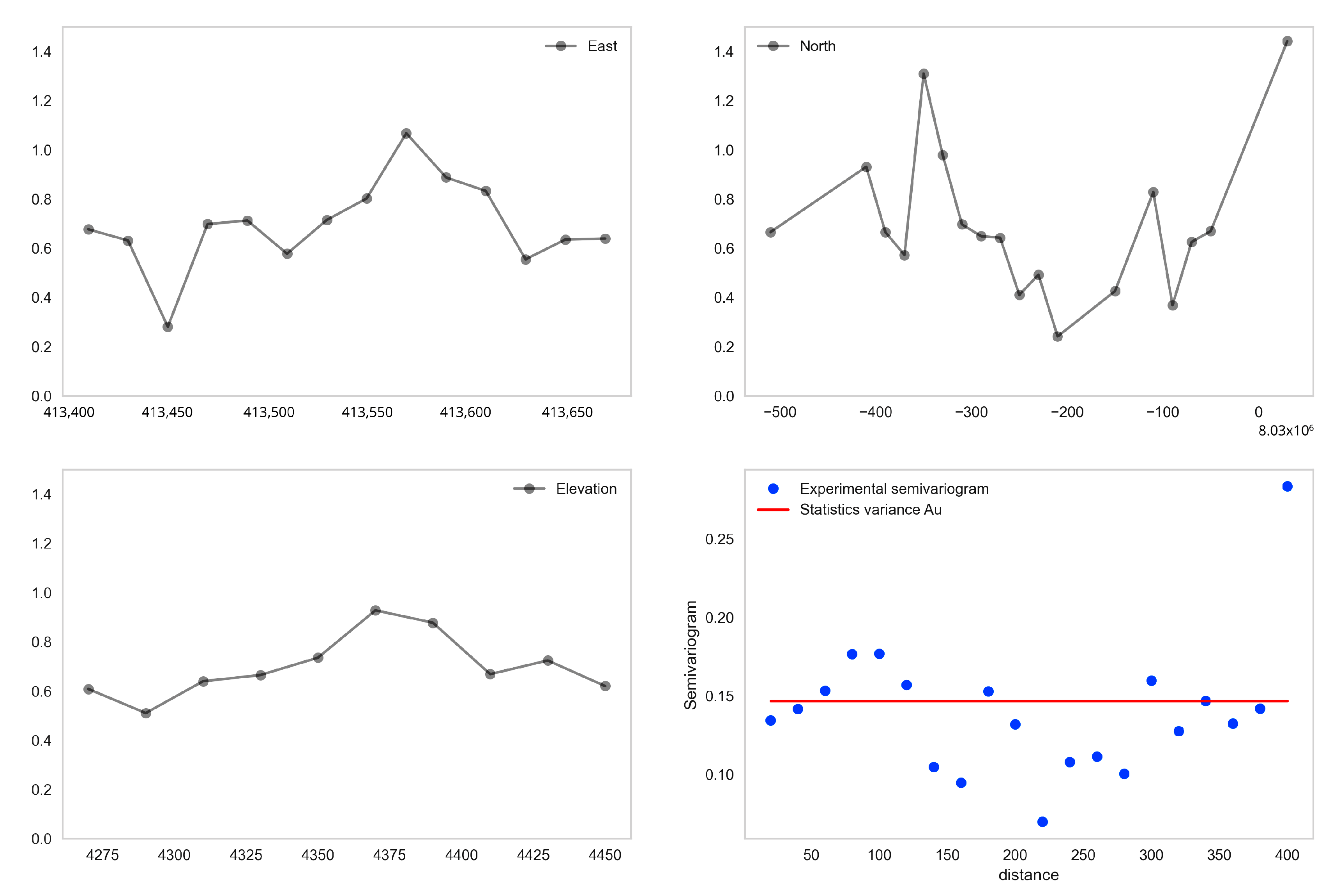
Finally, the resulting groups, which are ultimately the estimation domains, must be validated. Coombes [
22] proposes a simple variance review approach based on grids as a minimum requirement for the validation of estimation domains. However, in this study, we use the semivariogram estimator additionally [
23] to detect spatial dependence. The following expression corresponds to the experimental semivariogram, which is an unbiased estimator for the semivariogram:
where
Z is a variable of interest known in
;
is the number of pairs of variables at distance
h.
3. Case Study
The objective of this research is the validation of the k-prototype clustering method for the definition of geostatistical estimation domains through an application case. The available data set is the result of 131 diamond drill holes and 37 exploration trenches, carried out with the purpose of identifying, characterizing, and evaluating a hydrothermal gold deposit of high sulfidation, located in the province of Tacna, district of Palca, southern Peru. Gold is the most important economic metal for which the estimation domains are defined. The available variables are the following: gold grade (Au), silver grade (Ag), type of alteration, and mineral zone.
In
Figure 1, the complete process, from the selection of the variables, to the evaluation of the domains can be seen. Regarding the exploratory data analysis: the 1st step has the purpose of describing, relating, and cleaning the data coming from the drilling campaign (composites). In step 2, those features, both numerical and categorical, that affect the definition of domains are selected. After that, in step 3, the numerical features are standardized. In step 4, categorical features are converted into new binary type variables. In the 5th step, the algorithm
k-prototypes are applied in
n scenarios. After that, the optimal number of domains is selected (step 6). Finally, in step 7, it is evaluated if the domain is geostatistically estimable, through a variogram. The algorithm
k-prototypes is explained in Algorithm 1. The input of the algorithm is the set of
n data objects (
,
, ⋯,
), and the output is the number of clusters
k.
| Algorithm 1 Algorithm to determine the number of clusters k |
- 1:
procedurek-prototypes(, , ⋯, ) - 2:
Select k initial prototypes (cluster centers) randomly from the data set - 3:
Attribute each data point in the data set to its closest cluster center according to Equation ( 2) - 4:
Update the cluster centers position after each allocation - 5:
if the updated cluster centers are identical to the previous ones then - 6:
finish - 7:
else return to the beginning - 8:
end if - 9:
end procedure
|
Ag’s grade has both statistical correlation (76%) and apparent spatial similarity with Au’s grade. The geological attributes that control mineral grade are the mineral zone and the type of alteration (both categorical variables). The X, Y, and Z coordinates identify the centroid of each composite.
The mineral zone is an attribute that is presented in three categories: oxides, mixed, and sulfides. This attribute has a strong control over the mineral grade, and it is established as restrictive for grouping. This means that in the estimation domains that are defined, there cannot be a mixture of these zones. Thus, the clustering algorithm will be applied independently in each of them. In
Table 1, the descriptive statistics of Au (parts per million, ppm) are presented, and in
Figure 2 the isometric view of drill holes by mineral zones.
The behavior of the gold grade is inversely proportional to the depth of the deposit: the deeper the deposit, the lower the Au grade. The mixed transition zone (M2) is the area with less information and the most representative of the global average grade, while the oxide (M1) and sulfide (M3) zones have a similar amount of data and they present more extreme average Au grades; see
Table 1. In
Table 2, the contact analysis of Au is presented, where the following notation has been used: not applicable (NA), soft contact (SC), hard contact (HC).
In
Figure 3, it is observed that the mineral zones have independent distributions based on the gold grade; thus, they should be kept separate. The sulfide zone (M3) is the one that slightly presents a greater amount of changes in the slope. Therefore, a priori, it is an area that possibly should be divided into more groups of grades than M1 and M2, where two areas can be distinguished in each of the groups. Au presents a high positive asymmetry and kurtosis, describing an impoverished deposit, where the accumulation of grades is concentrated in low values. In this type of distribution, it is not possible to detect the existence of populations that coexist in a histogram. For this reason, a log-normal transformation is applied to the Au grades (
Figure 4). It is possible to observe at least two populations that are very different in size per each mineral zone.
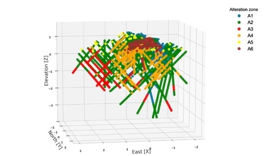
On the other hand, the type of alteration which is the second geological attribute and that directly influences the work of the clustering algorithm, is presented in six categories; see
Table 3. In
Figure 5, the isometric view of drill holes by type of alteration is presented, and in
Table 4, the contact analysis of Au by type of alteration is shown. The same notation as in
Table 2 has been used; and the case of no physical contact has been denoted by NC. The coverage (A5) does not have enough samples to evaluate contact.
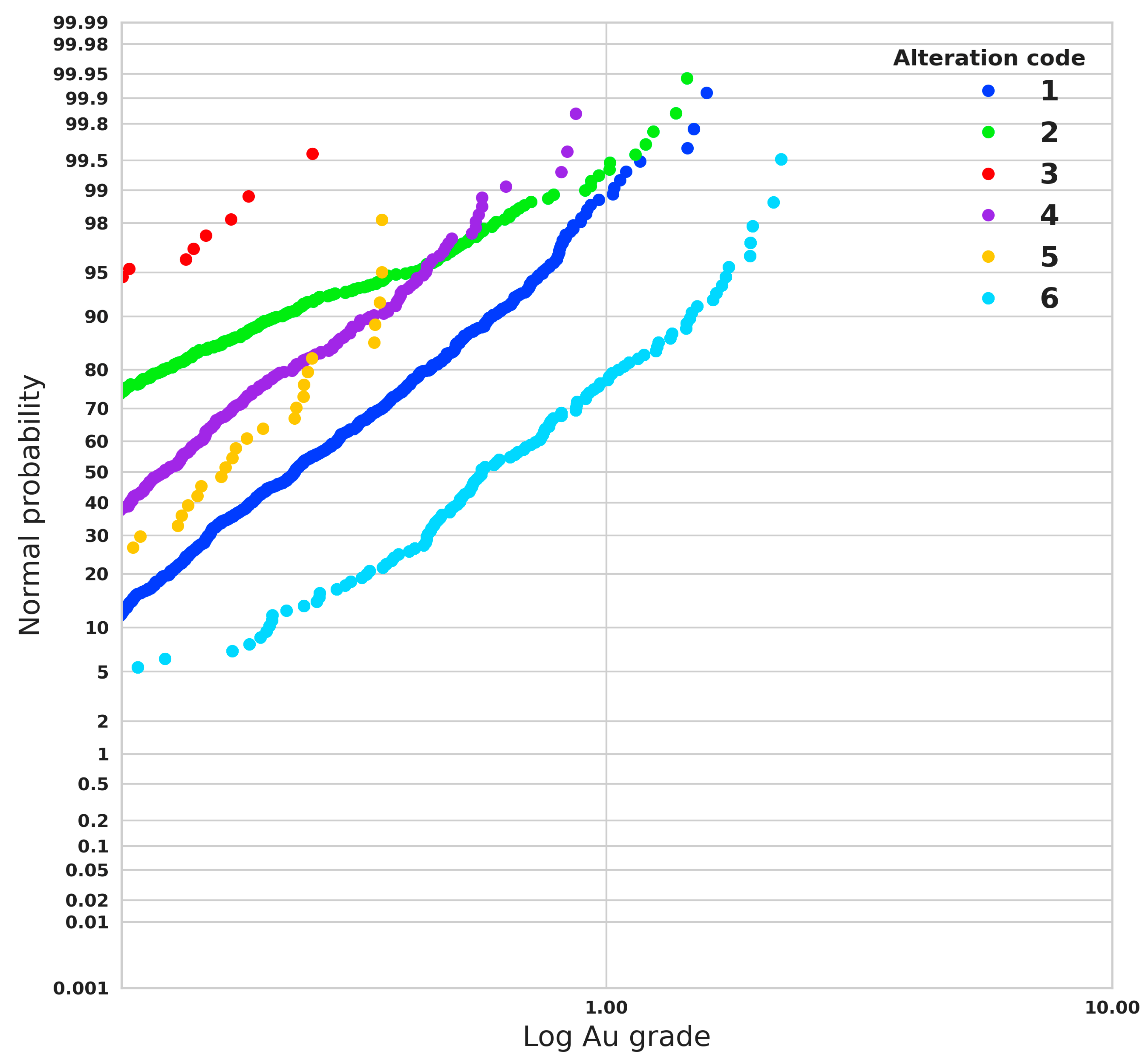
The predominant alteration in the deposit is the argillic type (A1 and A2), covering the 72% of the sample. Then, in terms of abundance, silica follows (A4) covering the 16%, and finally chloritization (A3), vuggy (A6), and coverage (A5) being 6%, 5%, and 1%, respectively. Each of these categories maintains a control over the Au grade. See, for example, the mineral enrichment that occurs in A6 versus the mineral depletion of A3, in
Table 3. In
Figure 6 the normal probability plot for each alteration can be seen.
The numeric variables Au and Ag will contribute to the grouping, because, as mentioned above, they are similar in their spatial arrangement and have an apparent statistical correlation, which would add weight in the definition of homogeneous domains for Au. On the other hand, and unlike similar studies, the spatial coordinates X, Y, and Z will not be included due to the fact that these would influence excessively a spatial grouping, leaving the main variable of interest in the background and losing homogeneity by domain.
Au and Ag are variables that have different scale and variance. Therefore, they are standardized for a correct contribution of information. The z-score transformation has been applied, obtaining two transformed variables of mean 0 and variance 1. Regarding the two categorical variables, only the alteration will provide information in the grouping, which is the one that has the greatest control over Au. The three categories of the mineral zone are presented as independent scenarios where the grouping takes place.
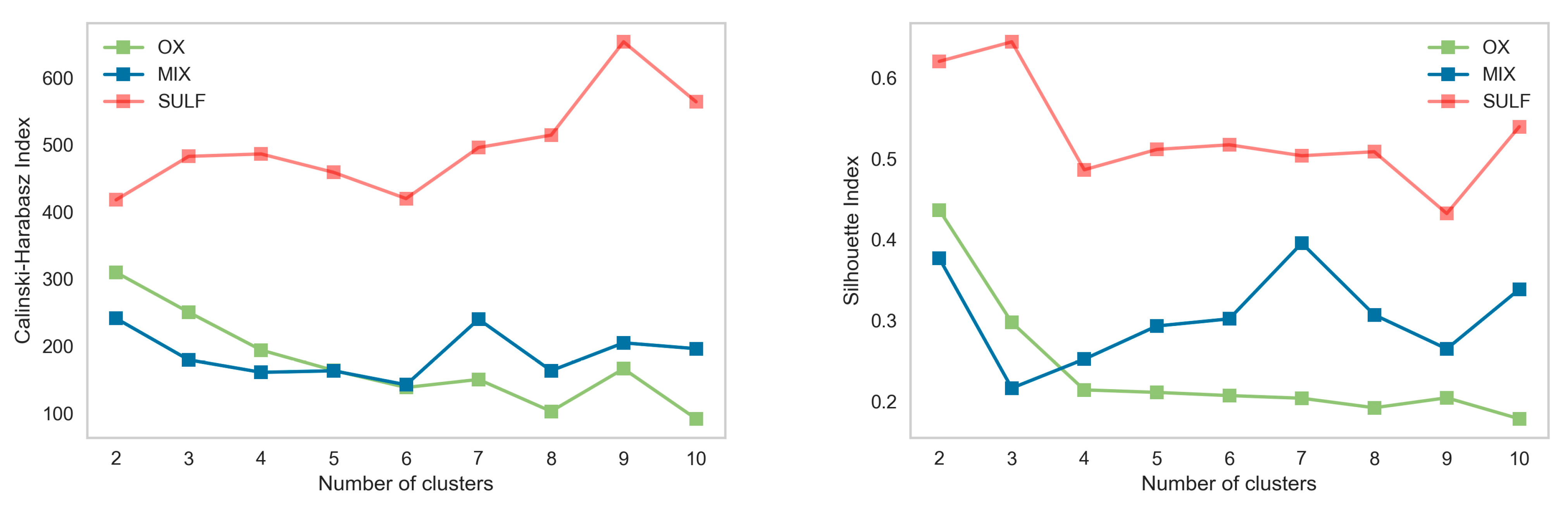
The
k-prototype algorithm is applied in nine different scenarios, ranging from
to
, for each of the mineral zones and using three variables: Au, Ag, and alteration. The
k scenarios are evaluated using the Calinski–Harabasz index and the silhouette coefficient, see
Figure 7.
For oxidized and mixed minerals, both approaches have a higher score when
. For sulfides,
is presented as the best alternative. The latter is related to the populations detected in this mineral zone in the descriptive stage. The method
k-prototypes recommends seven domains, as shown in
Table 5: two domains for the mineral zone M1, the other two domains for M2, and three domains for M3.
This methodology favors the homogeneity of the variable of interest and the heterogeneity between domains, unlike the traditional methodology which does not mix, a priori, alterations by mineral zone. Thus, a partial mixture between alterations is produced. In the case of the mineral oxide zone (M1), alteration A3 and A5 are not part of the D2 domain. This is because these type of alterations have a low concentration grade in Au. This is the reason why within the oxides, the domain D1 represents the group of low grades, and D2 high grades.
The same situation occurs with mixed minerals (M2), where the D3 domain, the first in its area, does not contain either A3 or A5 alterations (groups of low grades), and the domain D3 domain has higher grades. In the case of sulfur minerals (M3), three domains are defined. The smallest domain (D7) concentrates a group of high grades, similar to those of the D2 domain of oxides, with the difference that D7 is a domain with poor information, and in which the alterations A1 and A2 interact most, being the ones with the highest grade. This fact demonstrates that the categorical variable alteration weighs in the grouping, since it controls the behavior of Au and provides the geological character required in the definition of domains. See the boxplot by estimation domain in
Figure 8.
The domains D1–D6 present spatial continuity, which can be seen in the omnidirectional semivariograms of
Figure 9,
Figure 10,
Figure 11,
Figure 12,
Figure 13 and
Figure 14. They also have a local stationarity that is sufficient to validate the use of the geostatistical model.
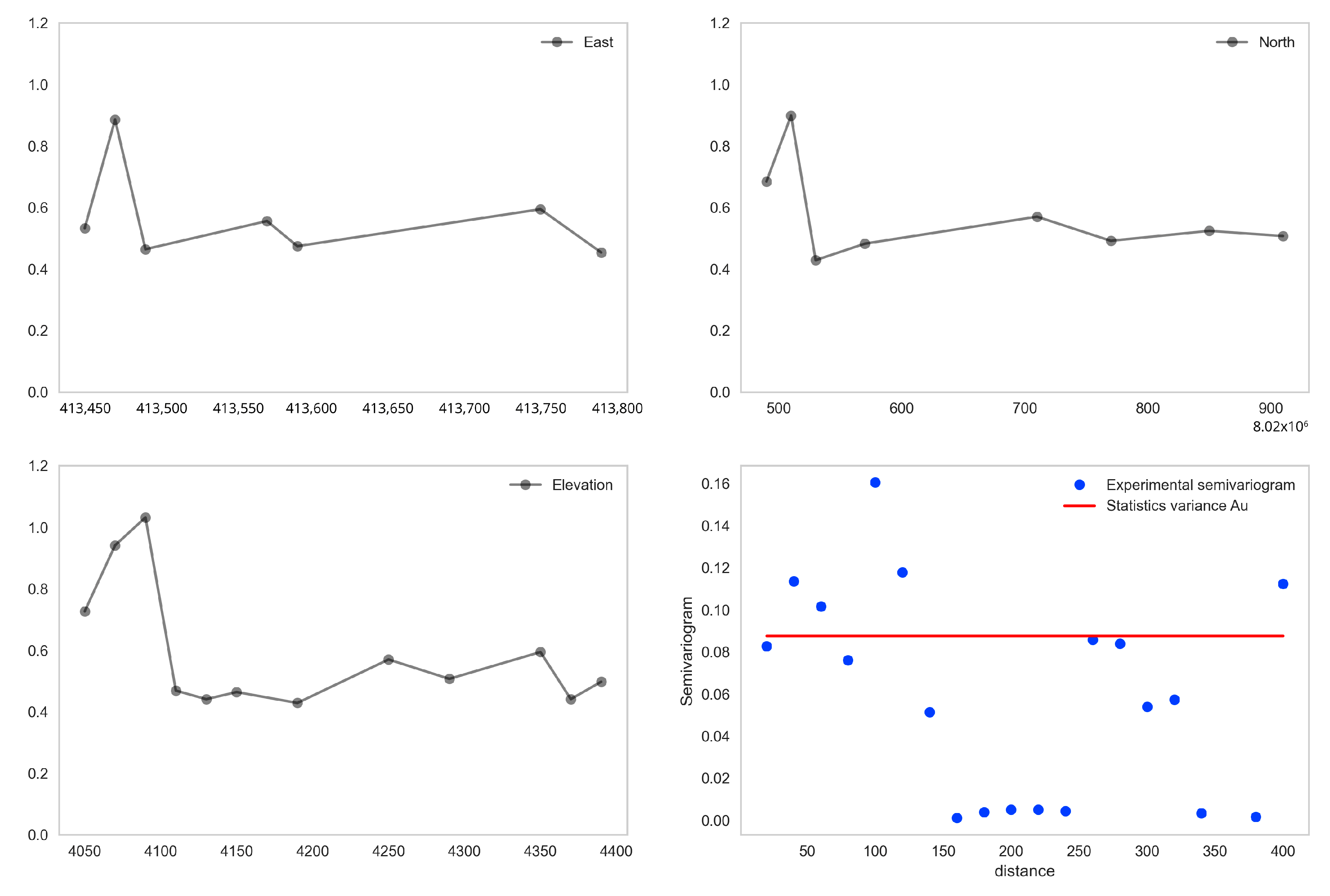
As mentioned above, the D7 domain recommended by this methodology is questionable, since it contains a very low amount of data corresponding to a mineral enrichment in the sulfide zone. The algorithm detects this anomaly and it separates, which makes difficult the variographic modeling, and therefore, the geostatistical estimation. This is evidenced in
Figure 15, where the drift graph and the omnidirectional semivariogram for the aforementioned domain are presented. A solution to this problem is to incorporate the domain D7 into another one in the sulfide zone, omitting its information when making the spatial continuity model.
4. Conclusions
In this study, the implementation of an unsupervised machine learning-based approach was evaluated using a multivariate clustering algorithm. The main goal of this research was to implement and test successfully a previously non-applied alternative method to define the assessment domain that meets the principles of geostatistical assessment. The traditional approach used to define the area of mineral estimation is based on integrated geological and statistical studies, where geological understanding and human intervention dominate. The traditional approach is relatively slow as its steps need to be carried out and supervised using expert personnel. As well, the behavior of mineral properties is not always uniform, it may present stationarity, so its spatial structure can be interpreted in different ways, as geological domains are strongly dependent on geological attributes. Thus, the aim of the initiative presented in this practical approach was to reduce both the time factor for which traditional methods are criticized, and their subjectivity compared to the traditional methods.
The automatic grouping approach presented herein has shown satisfactory results in terms of time, resources used, and quality of results. The results obtained by the algorithm k-prototypes are consistent with the exploratory data analysis, where information regarding statistically independent populations for gold grade for each mineral zone is captured. By being able to mix numeric and categorical variables, the grouping incorporates the geological and spatial character from the attributes that maintain control over the mineral grade. The suggested domains meet the requirements to be modeled geostatistically, making it possible to advance in the estimation stage.
As limitation of the proposed initiative, we can say that this unsupervised automatic grouping approach does not depend solely on the algorithm. It must also consider a correct selection of variables, a preprocessing of these, the configuration of the initialization parameters, the number of scenarios to be evaluated, the evaluation methods, and the interpretation of the results weighing the geological sense with the sufficient degree of stationarity. Therefore, the approach proposed in this study does not replace the traditional methodology, but it is presented as a more efficient comparative alternative or complement in terms of time and homogeneity by domains, at the expense of making the mixture of categories by geological attribute more flexible.
The research has awakened the interest of Aingura IIoT for future developments in this line, which is a company that designs Industrial Internet of Things (IIoT) solutions for the industry. As suggested by practitioners from this company, further research will be oriented to the improvement of the approach in terms of the aforementioned variable selection, preprocessing, initialization and evaluation stages, to obtain a less technician-dependent tool.


