Recent Advances in Stochastic Gradient Descent in Deep Learning

Abstract

In the age of artificial intelligence, the best approach to handling huge amounts of data is a tremendously motivating and hard problem. Among machine learning models, stochastic gradient descent (SGD) is not only simple but also very effective. This study provides a detailed analysis of contemporary state-of-the-art deep learning applications, such as natural language processing (NLP), visual data processing, and voice and audio processing. Following that, this study introduces several versions of SGD and its variant, which are already in the PyTorch optimizer, including SGD, Adagrad, adadelta, RMSprop, Adam, AdamW, and so on. Finally, we propose theoretical conditions under which these methods are applicable and discover that there is still a gap between theoretical conditions under which the algorithms converge and practical applications, and how to bridge this gap is a question for the future.

1. Introduction

Deep learning is of great interest in such fields as healthcare, astronomy, and information science, where data are transformed into knowledge and processed intelligently. It is a data-driven information-mining technology that can process massive amounts of data. With the exponential growth of data, the traditional gradient descent method can no longer effectively solve large-scale machine learning problems. There are two types of common methods, and one is to use as many training samples as possible but perform only a tiny number of calculations per sample. The other is to take a small portion of the data for high-intensity calculations. The paper [1] proposes that the former method is more efficient, and its standard optimization algorithm is stochastic gradient descent (SGD).

With the rapid update and development of neural networks, gradient descent algorithms have received extensive attention from the academic community. In Pytorch, torch.optim is an optimizer package supporting the most common optimization algorithms, including SGD, Adagrad, Adadelta, RMSprop, Adam, AdamW, and so on. The stochastic optimization methods have been added to the PyTorch optimizer and are widely used to solve deep-learning problems [1,2,3].

This article discusses existing algorithms for neural networks and their typical applications in large-scale machine learning and deep learning. The main contributions of this paper are summarized as follows:

(1)

Introducing the optimization problem for large-scale data and reviewing the related models of deep learning.

(2)

Providing a review and discussion on recent advances in SGD.

(3)

Providing some applications, open issues, and research trends.

To the best of our knowledge, there are only a few SGD-related preprinted surveys [1,4,5,6]. Compared with them, our contribution does the following:

(1)

Summarizes SGD-related algorithms from machine learning and optimization perspectives. Worth mentioning are the proximal stochastic methods, which still needed to be summarized hitherto.

(2)

Provides the mathematical properties of models and methods.

(3)

Discusses the gap between theory and applications.

The remainder of this work describes several common deep-learning applications of SGD and then presents the many types of stochastic gradient descent. Finally, we summarize this article and discuss various unresolved concerns and research directions.

2. Application

The SGD algorithm has been applied to tasks such as natural language processing (NLP), visual data processing, and speech and audio processing in deep learning. We introduce the different tasks of deep learning and list some practical applications of the SGD algorithm in these significant fields.

2.1. Natural Language Processing

Natural language processing (NLP) aims to enable computers to interpret, process, and understand human language.

Many studies have been put forward for different NLP tasks. For sentiment analysis, the recursive neural tensor network (RNTN) with tensor-based combinatorial functions was proposed in [7], which can be used to determine which phrases are positive and which are negative. This method uses the optimizer AdaGrad when generating the model. To address the issue of text generation, the paper [8] proposes a hierarchical approach based on CNNs and a fusion architecture with the pre-trained language model whose optimizer is NAG. For machine translation, Ref. [9] introduced a novel deep transition architecture called DTMT. For paraphrase identification, the authors of [10] utilized mini-batch SGD for solving the unfolding recursive autoencoders (RAEs). Both word- and phrase-level similarities are measured simultaneously using syntactic trees to develop the feature space. A recently suggested deep-learning architecture called attention-based CNN (ABCNN) aims to identify the dependency between two phrases [11] and is optimized by Adagrad. BERT [12] is a multi-layer bidirectional transformer encoder that can be used in large-scale sentence-level or token-level tasks, whose optimizer is Adam.

2.2. Computer Vision

Computer vision aims to allow computers to imitate human eyes to recognize, track, and measure objects [13].

For image classification tasks, LeNet-5 [14] and AlexNet [15] are the first proposed convolutional models. VGGNet [Karen 204], ResNet [Kaiming 205], and ResNeXT [Saining 206] were later developed as improved methods. For object detection tasks, R-CNN [16], YOLO [17], and R-FCN [18] were proposed. For video processing tasks, the authors of [19] replaced the convolutions in EfficientDet and HRNet with skip-convolutions without any loss of accuracy while reducing the computational cost. The commonly used solution operators for these models are SGD and SHB. A novel recurrent convolution network (RCN) model was proposed in [20], which combines RNN and CNN. The paper [21] presents a conditional diffusion model for image-to-image translation tasks. SR3 developed a denoising diffusion probabilistic model for super-resolution [22]. These three models use Adam as the optimization solver.

2.3. Speech and Audio Processing

The goal of speech recognition technology is to allow computers to convert speech signals into corresponding text through the processes of recognition and understanding [23].

For the speech emotion recognition (SER) task, the authors of [24] proposed a feedforward artificial neural network using a single hidden layer for discourse-level classification, whose optimizer is mini-batch SGD. The authors of [25] proposed an attentive CNN model on feature learning for speech emotion recognition. A new architecture for semi-supervised cross-modal knowledge was proposed to constrain the consistency of the transfer from visual to audio modalities [26]. For the enhancement (SE) task, the authors of [27] proposed a network that simulates complex-valued computation and is constructed to train complex targets more efficiently. These three models use Adam as the optimization solver.

2.4. Others

For crisis response tasks, the authors of [28] offered a novel approach paired with online learning capabilities. It effectively identifies future catastrophes at the phrase level using tweets and identifies the observed disaster types for crisis-response activities. The optimizer for this model is Adadelta. For disease prediction, the authors of [29] utilized a CNN-based autoencoder to predict cellular breast cancer, whose optimizer is SHB.

Table 1. Summary of applications.

Application	Ref.	Model	Method
Natural Language Processing	[7]	Recursive Neural Tensor Network (RNTN)	AdaGrad
	[8]	hierarchical approach based on CNNs	NAG
	[9]	Deep Transition RNNbased Architecture for NMT (DTMT)	Adam
	[10]	Unfolding recursive auto-encoders (RAE)	Mini-batch SGD
	[11]	Attention-Based CNN (ABCNN)	Adagrad and weight decay
	[12]	BERT	Adam
Visual Data Processing	[14]	LeNet-5	SGD
	[15,30,31,32]	AlexNet/ VGGNet/ ResNet/ ResNeXT	SHB and weight decay
	[16]	Region-based CNN (RCNN)	Minibatch SGD
	[17]	YOLO (an object detection model)	SHB and weight decay
	[18]	Region-based Fully Convolutional Networks (R-FCNs)	SHB and weight decay
	[19]	Skip-Convolutions Networks	SGD with momentum 0.9
	[20]	Recurrent Convolution Networks (RCN)	Adam
	[22]	Super-Resolution via Repeated Refinement (SR3)	Adam
	[21]	a conditional diffusion model	Adam
Speech and Audio Processing	[24]	Extreme Learning Machine (ELM)	Mini-batch SGD
	[25]	the attentive CNN	Adam
	[27]	DCCRN	Adam
	[26]	A semi-supervised cross-modal network	Adam
Other	[28]	A CNN-based method	Adadelta
	[29]	A CNN-based Auto encoder	SHB and adaptive learning rate

shows a summary of the applications of the deep-learning networks, their architectures, and the stochastic methods used.

3. Stochastic Methods for Deep Learning

Training a neural network is an optimization procedure that involves determining the network parameters that minimize the loss function. These models require massive datasets and many model parameters to be tuned. In the age of artificial intelligence, finding the optimal method to handle enormous amounts of data is inspiring and challenging.

Stochastic gradient descent (SGD) [33] is simple and successful among machine learning models. A great deal of work has been suggested in the past several years to solve optimization problems or improve optimization approaches in machine learning.

Given the train data $(x_i,y_i)$ with $i=1,2,\dots n$, the general form for optimization problem is:

$$\underset{w}{min}\ell \left(w\right):=\frac{1}{n}\sum _{i=1}^n{\ell }_i(h(x_i;w),y_i),$$

(1)

where w represents the weights of the model, h is prediction function, and ${\ell }_i$ is the loss function.

There are some simplified notations. A random seed $\xi$ is used to represent the sample (or a group of samples). Furthermore, f is the combination of the loss function ℓ and the prediction function h, so the loss is rewritten as $f(w,\xi )$ for any given pair $(w,\xi )$.

Some fundamental optimization algorithms for minimizing risk are given in the rest of this section.

3.1. Batch Gradient Descent

To update the weights w, the gradient descent technique computes the gradient of the loss function. The learning rate $\eta$ determines the extent of each iteration, influencing the number of iterations required to get the ideal value. The batch gradient descent [34], also known as complete gradient descent, uses all samples to update parameters. The following steps are alternated until the algorithm converges:

$$w^{+}=w-\frac{\eta }{n}·\sum _{i=1}^n\nabla f(w;{\xi }_i),$$

where w is the result of the previous iteration.

A cycle of training the entire dataset is called an "epoch," and batch gradient descent stops updating at the end of all training epochs. One update of the dataset needs to calculate all of their gradients. Batch gradient descent is prolonged on large-scale data and intractable for datasets that do not fit in memory. Thus, it also does not suit online learning. However, this method decreases the frequency of updates and results in a stable solution.

The batch gradient descent method is easy to use. If the objective function is convex, the solution is the global optimum. In convex problems, batch gradient descent has a linear convergence rate and is guaranteed to converge to a local minimum in non-convex issues.

Common examples of gradient descent are logistic regression, ridge regression, and smooth hinge loss. Hinge loss is not differentiable. Thus, we can use its subgradient. However, in deep learning, too much layering causes an unstable gradient.

3.2. SGD

A variant of the gradient descent algorithm is stochastic gradient descent (SGD). Instead of computing the gradient of $\mathbb{E}\left[f(w;{\xi }_i)\right]$ or $\frac{1}{n}{\sum }_{i=1}^n{f}_i(w;{\xi }_i)$ exactly, it only uses one random sample to estimate the gradient ${\zeta }_i$ of $f_i(w;{\xi }_i)$ in each iteration. Batch gradient descent conducts redundant calculations for large-scale problems because it recomputes the gradients of related samples before each parameter changes, whereas SGD does only one computation per iteration. Algorithm 1 contains the whole SGD algorithm. It is simple to use, saves memory, and can also be suited to online learning.

Algorithm 1: Stochastic gradient descent (SGD) [33].

1: Input: learning rate ${\eta }_t>0$. 2: Initialize$w_0\in {\mathbb{R}}^d$, $t=0$. 3: while Stop Criteria is True do 4:    Sample ${\xi }_i\sim P$ with $i\in 1,2,\dots ,n$ 5:    ${\zeta }_i=\nabla f_i(w_t;{\xi }_i)$ 6:    $w^{+}=w-{\eta }_t·{\zeta }_i$ 7:    $t=t+1$ 8: end while

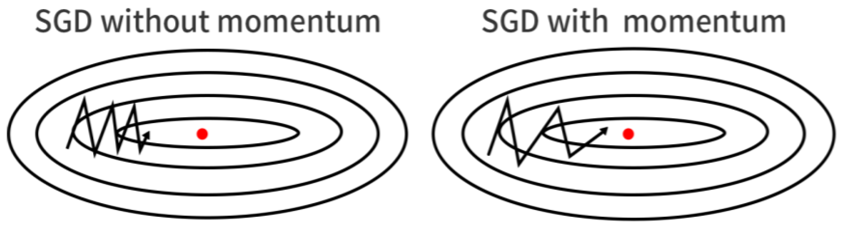
Stochastic gradients are unbiased estimates of the real gradient. Add random noise with a mean of zero to gradient descent to simulate SGD. Figure 1 shows a comparison of noiseless and noisy: SGD training with a single example causes fluctuations, making iterative trajectories tortuous and slow at converging.

During backpropagation, the iterations are updated by the chain-derivative rule, which can easily lead to unstable gradients. Specifically, if the multiplier is much larger than one, the update result increases rapidly with the iterative process, and the gradient explodes. If the multiplier is much less than one, the result drops off rapidly with iterations, with gradient decay. To solve the gradient instability and avoid the gradient effect by the scale of the weight, the authors of [35] proposed batch normalization (BN), which is related to the formulation of the activation function.

The cost of SGD is independent of sample size, allowing it to attain sublinear convergence rates in convex problems [36]. SGD shortens the update time when dealing with multiple samples and eliminates some computational duplication, which greatly speeds up the computation. SGD can reach the fastest convergence speed in the strong convex problem [33,37]. When the condition of the optimization problem is weaker than the strong convex condition, SGD also has a high convergence rate. The authors of [38] introduced an asynchronous parallel strategy that may achieve linear convergence under an essential strongly convex condition. Ref. [39] proves that when the Polyak–Lojasiewicz condition is satisfied, the iteration point converges linearly to a stable point when it falls into its neighborhood. Moreover, the paper [40] proves that if the PL condition is satisfied, SGD finds the global solution.

Some fundamental improvements for SGD in the optimization process [41] include increasing speed and reducing fluctuation. Choosing a proper learning rate can improve optimization speed. A large learning rate may cause instability near the optimal solution without convergence; otherwise, it results in a slower convergence rate and time-consuming updating. Some acceleration methods take another small step in a particular direction to improve convergence speed. These fundamental improvement methods are provided in detail in the remaining sections.

3.3. Mini-Batch SGD

Mini-batch SGD capitalizes on the benefits of both the gradient descent algorithm and SGD [33]. It is also the most common implementation of the stochastic method used in deep learning. In each iteration t, mini-batch SGD uses randomly and uniformly sampled small-batch training data ${\mathcal{I}}_t$ to compute the gradient, and $|{\mathcal{I}}_t|$ is the batch size. When acquiring small batches, it is possible to do put-back sampling with or without put-back. The detailed steps are shown in Algorithm 2.

Algorithm 2: Mini-batch SGD [33].

1: Input: learning rate ${\eta }_t>0$, 2: Initialize$w_0\in {\mathbb{R}}^d$, $t=0$. 3: while Stop Criteria is True do 4:    $z_t\leftarrow \nabla f_{{\mathcal{I}}_t}\left(w_t\right)=\frac{1}{|{\mathcal{I}}_t|}{\sum }_{i\in {\mathcal{I}}_t}\nabla f_i\left(w_t;{\xi }_i\right)$ 5:    $w_{t+1}=w_t-{\eta }_t·z_t$ 6:    $t=t+1$ 7: end while

It is easy to see that gradient descent and SGD are two special examples of mini-batch SGD [42]. SGD trains fast but introduces noise, whereas gradient descent trains slowly but computes gradients accurately. The authors of [43] proposed a dynamic algorithm that converges linearly to the neighborhood of the optimal point under strongly convex conditions. The authors of [44] presented a data selection rule that is such that a linear convergence rate can be achieved when updating with mini-batch SGD under the assumption of strong convexity or strong quasi-convexity.

The work [42] proposes an approximate optimization strategy by adding $l_2$ norm penalty term in each batch training. The method solves the subproblem

$$\underset{x}{min}\frac{1}{|{\mathcal{I}}_t|}\sum _{i\in {\mathcal{I}}_t}{f}_i(w;{\xi }_i)+\frac{{\gamma }_t}{2}{∥w-w_{t-1}∥}^2,$$

(2)

where ${\mathcal{I}}_t$ is a subset of $\{1,2,\dots ,n\}$ and ${\gamma }_t>0$. We provide a subtle change which uses

$$z_t\leftarrow =\frac{1}{|{\mathcal{I}}_t|}\sum _{i\in {\mathcal{I}}_t}\nabla f_i\left(w_t;{\xi }_i\right)+{\gamma }_t\left(w_t-w_{t-1}\right)$$

instead of step 4 in Algorithm 2.

However, the training result starts to deteriorate when the mini-batch’s size exceeds the threshold, and simply scaling the step size does not help. The authors of [45] showed that the large batch size could maintain generalization performance. In addition, choosing a batch size between 2 and 32 [46] is suitable for optimal performance. When the batch size needs to be larger, it will have better parallelism [47].

Table 2. The comparison of SGD, GD, and mini-batch SGD.

Method	Adv/Disadv	Description	Convergence	Numerical Experiment
GD	Adv: Reduce the number of iterations, stable	Select all samples.	convex: convergence to a global minimum	The ridge/logistic regression, smooth hinge loss.
	Cons: Slow, not suitable for online learning		Non-convex: convergence to a local minimum	The neural network may cause an unstable gradient.
SGD [33]	Adv: easy to implement, memory-efficient and suitable for online learning. Disadv: fluctuate, unstable, high variance.	Select one of the samples randomly.	Essential strong convex: linear convergence to the global optimal solution	The four-parameter affine-linear network; regression + nonconvex regularizer.
			PL condition: Linearly converge to a neighborhood of a stationary point → Sublinearly converge to the global optimal solution
			Nonconvex smooth: finds a stationary point
MSGD [33]	The compromise between SGD and GD	Select a small batch of the samples randomly.	Strong convex:a dynamic Mini-Batch size SGD linearly converges to a neighbourhood of the optimal point	$L_2$ regularized ridge regression
			Strong pseudo-convex: linear convergence

shows the comparison of SGD, GD and mini-batch SGD.

4. Variance-Reducing Methods

Due to the significant variance in SGD, it converges slowly. To improve this problem, many methods usually compute the full gradient after a certain period to reduce the variance. The stochastic average gradient (SAG) method [48], which is shown in Algorithm 3, makes the convergence more stable [49].

Algorithm 3: Stochastic average gradient (SAG) [48].

1: Input: learning rate $\eta >0$, 2: Initialize$w_0\in {\mathbb{R}}^d$, $d=0$, $z_i=0\mathrm{for}i=1,2,\cdots ,n$. 3: for$t=0,1,\dots$do 4:    Sample ${\xi }_i\sim P$ with $i\in 1,2,\dots ,n$ 5:    $d=d-z_i+\nabla f_i(w_t;{\xi }_i)$ 6:    $z_i=\nabla f_i(w_t;{\xi }_i)$ 7:    $w_{t+1}=w_t-{\eta }_t·d$ 8: end for

The SAG method needs to store the gradient of each sample. Additionally, this method only applies to smooth and convex functions, not non-convex neural networks. The authors of [36] proposed the stochastic variance reduced gradient (SVRG), method as shown in Algorithm 4. SVRG performs gradient replacement every m iteration, instead of computing the full gradient.

Many improved variants of variance-reduction methods have emerged, such as SDCA [50], MISO [51], and S2GD [52]. A novel method SARAH combines some good properties of existing algorithms [53]. Lots of studies improved SARAH in different aspects, resulting in algorithms such as SARAH+ and SARAH++. It is not necessary for careful choices of m sometimes [54]. In general, the fundamental SGD variants perform at a sublinear convergence rate. On the other hand, all of the preceding approaches, except S2GD, may achieve a linear convergence speed on severely convex problems. S2GD established linear convergence of expected values and achieved linear convergence in practice. The approaches described above can provide quick convergence to high accuracy by maintaining a large constant step size. To guarantee a linear convergence rate, they are always applied to $l_2$ regularized logistic regression problems [53,55].

Without theoretical results, the authors of [56] showed SVRG’s effectiveness at addressing various convex and non-convex problems. Moreover, experiments [36,57] showed the superior performance of SVRG to non-convex neural networks. However, applying these algorithms to the higher-cost and deeper neural nets is a critical issue that needs to be further investigated.

Table 3. Summary of the variance-reducing methods.

Method	Adv/Disadv	Description	Convergence	Numerical Experiment
SAG [48]	Adv: reduce variance and improve convergence speed Disadv: SAG is only suitable for convex smooth functions.	Each iteration calculate the gradient using only one sample. After the all sample are used once, it means the full gradient is computed. It needs to record the gradient of each sample, so it take up too much space.	Strong convex: Except for S2GD, the others all linearly converge to the global optimal. S2GD achieves linear convergence on the expected value of the objective function. However, for numerical experiments, it achieves the linear convergence.	$L_2$ regularized logistic regression problems
SVRG [36]		Calculate the full gradient in every m iterations instead of in each iteration
SARAH [53]		Calculate the full gradient in every m iterations instead of in each iteration
Others		S2GD, SDCA, MISO [50,51,52]

shows these variance-reducing methods. Subsequent sections provide more strategies for improving the stochastic algorithms.

Algorithm 4: Stochastic variance reduced gradient (SVRG) [36]

1: Input: learning rate $\eta >0$, and the inner loop size m. 2: Initialize${\tilde{w}}_0\in {\mathbb{R}}^d$. 3: for$s=1,2,\dots ,$do 4:    $\tilde{w}={\tilde{w}}_{s-1}$ 5:    $u=\frac{1}{n}{\sum }_{i=1}^n\nabla f_i\left(\tilde{w};{\xi }_i\right)$ 6:    $w_0=\tilde{w}$ 7:    for $t=1,\dots ,m$ do 8:      Sample ${\xi }_i\sim P$ with $i\in 1,2,\dots ,n$ 9:      $w_t=w_{t-1}-\eta \left(\nabla f_i\left(w_{t-1};{\xi }_i\right)-\nabla f_i(\tilde{w};{\xi }_i)+u\right)$ 10:    end for 11:    Set ${\tilde{w}}_s=w_m$ or ${\tilde{w}}_s=w_t$ with t chosen uniformly at random from $\{0,1,\dots ,m\}$ 12: end for 13: Output:${\tilde{w}}_s$

5. Accelerate SGD

SGD methods can quickly get stuck in saddle points on highly non-convex loss surfaces. At this time, SGD will oscillate and will not escape for a long time. The momentum [58] and Nesterov accelerated gradient [59] descent (NAG) are standard accelerating technologies replacing the traditional gradient method. This section introduces these accelerated technologies and their improvements.

5.1. Momentum

The concept of momentum comes from physical mechanics; it simulates the inertia of an object. As shown in Figure 2, the gradient oscillates vertically in a certain direction. A simple way to overcome the weakness is to maintain the gradient in the horizontal direction and suppress the gradient in the vertical direction.

It is similar to pushing a ball down in hill: the heavy ball accumulates momentum along the main direction of downhill, getting to the bottom of the hill faster and faster. This method is therefore also called the heavy ball method (HB) and is formulated as follows:

$$\begin{array}{c}{v}_t=\theta v_{t-1}+\alpha {\nabla }_{w}f\left(w\right),\\ w=w-v_t.\end{array}$$

(3)

where $\theta ,\alpha >0$.

The momentum method can speed up the convergence when the learning rate is small, as it is when dealing with high curvature, small gradients, and noisy gradients [58]. Moreover, the search process can converge more quickly [60].

The stochastic heavy ball method (SHB) converges sublinearly without the convexity assumption in [61]. For the specialized setting of minimizing quadratics, the SHB converges linearly at an accelerated rate in expectation [62]. When the objective function is strongly convex, a linear rate of convergence can be achieved using the HB method, toward the unique optimum, and when the objective function is smoothly convex, its Cesáro average can achieve a linear rate of convergence [63]. The sublinear convergence rate for weakly convex functions is established in [64]. The authors of [65] minimized the expected loss instead of the finite-sum loss and proved the objective function converges linearly. These theoretical results support robust phase retrieval problems, regression problems, and some CNNs. The class of quasi-strongly convex functions achieved the non-asymptotic optimal rates and global convergence with a unique minimizer [66]. The work of [67] demonstrates that SHB can improve the stability and generalization performance of the model. However, in the neighborhood of the nonconvex quadratic function’s stringent saddle point, HB can diverge from this point quicker than the GD [68]. There are still some shortcomings, such as the non-acceleration of SHB on SGD on some synthetic data [69].

Some work suggests that the common setting for this value is 0.9 [41]. An issue is determining the value of momentum factor $gamma$.

5.2. Nesterov Accelerated Gradient Descent

Instead of blindly following the slope, Nesterov accelerated gradient descent (NAG) [59] finds a more brilliant ball that knows where it slows down before speeding up again. The NAG updates the gradient of the future position. The gradient of the current situation is replaced by the next position, which is approximated to $w_t-\theta v_{t-1}$. NAG iterates the following equations for each step:

$$\begin{array}{c}{v}_t=\theta v_{t-1}+\alpha {\nabla }_{w}f\left(w_t-\theta v_{t-1}\right),\\ w=w-v_t,\end{array}$$

(4)

where $\theta ,\alpha >0$.

Figure 3 shows the HB(1-2-3) and NAG(1-4-5). HB first computes the current gradient (small blue arrow near point 1), then makes a big jump with momentum $v_k$ (big blue arrow) to point 2 (the real green arrow is the new momentum, $v_{k+1}$). The next step begins at point 2. HB computes the current gradient (small blue arrow near point 2), then makes a big jump with momentum $v_{k+1}$ (green broken arrow) to point 3, and the new momentum, $v_{k+2}$, is the purple arrow. NAG first makes a big jump with momentum $v_k$ (red broken arrow), measures the gradient, and then makes a correction (red line arrow near point 4). The next step begins at point 4. NAG makes a big jump with new momentum $v_{k+1}$ (yellow broken arrow) to measure the gradient and then makes a correction (red line arrow near point 5).

NAG+SGD (SNAG) converges sublinearly without a convex assumption [61]. The ASG method has been proved under the smooth, strongly convex assumption and has achieved a sublinear convergence rate [61]. The authors of [70] analyzed the convergence of variants of the NAG and SNAG, respectively. The SNAG weighs the speed of convergence and stability [67]. The authors of [71] demonstrated some limitations of NAG, such as the possibility of not converging or achieving speedup under finite sum conditions. These theoretical results were confirmed in models such as SVM and DNN. Considering only performance, SNAG performs well on many tasks, such as RNNs [72]. A new type of momentum named Katyusha momentum was proposed in [73]. However, if the step size is chosen as small, it leads to a slower convergence rate, which cancels out the benefit of the momentum term [69].

Table 4. Summary of the accelerate methods.

Method	Adv/Disadv	Description	Convergence	Numerical Experiment
HB [61]	Adv: Accelerate. Suit for the high curvature, small/noisy gradients Disadv: Do not know where to slows down and maybe slopes up again	Similar to pushing a ball down in hill: the heavy ball accumulates the momentum along the main direction of downhill, getting to the bottom of the hill faster and faster.	Strong convex: Converge linearly to the unique optimum	SVM, deep learning. NAG performs well for RNN without theoretical supports.
			Convex smooth: its Cesáro average has a linear convergence rate
			Strong pseudo-convex: global convergence to the unique minimizer
			Convex: Its except loss converges linearly
			Weak Convex: Sublinearly converges
			Some nonconvex quadratic function: diverge
NAG [61]	Adv: Know where should slows down.	NAG finds a smarter ball that knows where it slows down before slopes up again.	Smooth strongly convex:converges sublinearly to global minimizer
			Nonconvex: converges sublinearly to a stationary point
Others		Katyusha momentum [73]

shows these accelerate methods.

6. Adaptive Learning Rate Method

The learning rate is an essential hyperparameter for stochastic algorithms. If the learning rate is manageable, convergence may be achieved. The parameter update will be very time-consuming if the learning rate is too low. Unfortunately, the computed gradients may be sparse or may differ in magnitude in each dimension. This leads to some dimensions being very sensitive to the same learning rate. To solve this problem, an intuitive way is to choose different learning rates for each dimension. An adaptive learning rate method is proposed because it is time-consuming to select different learning rates for different dimensions manually. This section will talk about how to set an appropriate learning rate, which improves SGD and applies to the variant reduce methods and accelerate methods [2,74].

AdaGrad modifies the learning rate dynamically based on the gradients acquired in previous rounds. The updated formulas are as follows:

$$w_{t+1}=w_t-\frac{\eta }{\sqrt{G_t+ϵ}}·g_t$$

(5)

where $\eta$ is a default value of 0.01 and $g_t$ is the gradient. $G_t$ here is a diagonal matrix where each diagonal element is the sum of the squares of the past gradients. We take an example to explain how to compute $G_t$:

Given $g_1={(1,0,2)}^T$, $g_2={(3,4,0)}^T$, and $g_3={(0,5,6)}^T$, we have:

$$\begin{array}{cc}\hfill \sqrt{G_t+ϵ}=& \left(\begin{array}{ccc}\sqrt{1^2+3^2+ϵ}& 0& 0\\ 0& \sqrt{4^2+5^2+ϵ}& 0\\ 0& 0& \sqrt{2^2+6^2+ϵ}\end{array}\right)\hfill \\ & =\left(\begin{array}{ccc}\sqrt{10+ϵ}& 0& 0\\ 0& \sqrt{41+ϵ}& 0\\ 0& 0& \sqrt{40+ϵ}\end{array}\right)\hfill \end{array}$$

This computive fomulate of $G_t$ is the same in the following algorithms.

One significant advantage of AdaGrad is that it eliminates the need to adjust the learning rate manually. The approach may be used to solve sparse gradient issues. The settings update ineffectively when the algorithm no longer needs to learn anything new. Adagrad provides convex optimization sublinear convergence [75]. Adagrad is nearly certainly asymptotically convergent in the non-convex problems [76]. The authors of [77] provided robust linear convergence guarantees for either highly convex or non-convex functions that meet the Polyak–Lojasiewicz (PL) assumption for most minor squares problems.

This algorithm has a small cumulative gradient and a large learning rate in the first few rounds of training. However, as the training time increases, the incremental gradient becomes larger and larger, resulting in a learning rate that tends to zero, and the weights of the model may not be updated. Adadelta [78] and RMSProp [79] are two extensions of Adagrad to overcome its drawback. They focus on the gradients in a window over a period instead of accumulating all historical gradients. They are inspired by the momentum method, which uses an exponential moving average to calculate the second-order cumulative momentum. The process of them:

Adadelta:

$$E{\left[g^2\right]}_t=\gamma E{\left[g^2\right]}_{t-1}+(1-\gamma )g_t^2,$$

(6)

where $E\left[·\right]$ is the expectation. Then,

$$\Delta w_t=-\frac{\eta }{\sqrt{E{\left[g^2\right]}_t+ϵ}}{g}_t.$$

(7)

The update should have the same hypothetical units as the parameter.

$$\begin{array}{c}E{\left[\Delta w^2\right]}_t=\gamma E{\left[\Delta w^2\right]}_{t-1}+(1-\gamma )\Delta w_t^2,\\ RMS{[·]}_t=\sqrt{E{\left[{·}^2\right]}_t+ϵ},\\ \Delta w_t=-\frac{RMS{[\Delta w]}_{t-1}}{RMS{\left[g\right]}_t}{g}_t,\\ w_{t+1}=w_t+\Delta w_t.\end{array}$$

(8)

RMSProp:

$$E{\left[g^2\right]}_t=\gamma E{\left[g^2\right]}_{t-1}+(1-\gamma )g_t^2,$$

(9)

where $E\left[·\right]$ is the expectation. Then,

$$\begin{array}{c}\Delta w_t=-\frac{\eta }{\sqrt{E{\left[g^2\right]}_t+ϵ}}{g}_t,\\ w_{t+1}=w_t+\Delta w_t,\end{array}$$

(10)

where $\gamma$ is always set to 0.9, and a good default value for the learning rate $\eta$ is 0.001.

They are suitable for non-convex problems and end up oscillating around local minima.

Adaptive moment estimation (Adam) [2] is not only computationally efficient, but also memory-efficient, and it is suitable for large-scale data problems. Adam is a combination of adaptive learning rate and momentum methods:

$$m_t=\alpha m_{t-1}+\left(1-\alpha \right)g_t,v_t=\beta v_{t-1}+\left(1-\beta \right)g_t^2,$$

(11)

$m_t$ and $v_t$ are first moment and second moment of the gradients.

$$\begin{array}{c}{\widehat{m}}_t=\frac{m_t}{1-{\alpha }^t},{\widehat{v}}_t=\frac{v_t}{1-{\beta }^t},\\ w_{t+1}=w_t-\frac{\eta }{\sqrt{{\widehat{v}}_t}+ϵ}{\widehat{m}}_t,\end{array}$$

(12)

where $0<\alpha <1$ and $0<\beta <1$.

Due to its stable process, it is suited to non-convex problems in high-dimensional space. However, Adam and RMSProp are confirmed to be divergent in some scenarios via convex cases [80]. Considering the original schemes are convergent by using a full-batch gradient, the authors of [81] adopted a big batch size. The sublinear convergence rates of RMSProp and ADAM are provided in the non-convex stochastic setting by setting a specific batch size. These theoretical theories are helpful in the training of machine learning and deep neural networks, such as LeNet and ResNet [82].

Nadam combines Adam and NAG [83]. AdaMax gives a general momentum term, which replaces $\sqrt{{\widehat{v}}_t}+ϵ$ (can be seen as $l_2$ norm) with

$$\begin{array}{cc}\hfill u_t& ={\beta }^{\infty }{v}_{t-1}+\left(1-{\beta }^{\infty }\right){\left|g_t\right|}^{\infty }\hfill \\ & =max\left(\beta ·v_{t-1},\left|g_t\right|\right)\hfill \end{array},$$

which can be regarded as the $l_{\infty }$ norm.

AdamW [84] is an improved quality method using Adam’s $l_2$ regularization/weight decay, which avoids the negative effect of the interaction between $m_t$ and $v_t$.

$$\begin{array}{c}{\widehat{m}}_t=\frac{m_t}{1-{\alpha }^t},{\widehat{v}}_t=\frac{v_t}{1-{\beta }^t},\\ w_{t+1}=w_t-\eta \lambda w_{t-1}-\frac{\eta }{\sqrt{{\widehat{v}}_t}+ϵ}{\widehat{m}}_t,\end{array}$$

(13)

where $\eta ,\lambda >0$.

In addition, many modified versions of the above methods have been proposed, namely, AdaFTRL [85], AdaBatch [86], SC-MSProp [87], AMSGRAD [80], and Padam [88].

Table 5. Summary of the adaptive learning rate methods.

Method	Adv/Disadv	Description	Convergence	Numerical Experiment
AdaGrad [74]	Adv: Adaptively adjust the learning rate Disadv: As the gradient accumulates, the learning rate will become 0.	Adjusts the learning rate dynamically based on the historical gradient in the previous iterations.	Strongly convex/PL conditions: linearly converges	machine learning and deep neural networks, such as LeNet and ResNet
			Convex: sublinearly converges
			Smooth nonconvex: almost surely asymptotic convergent.
Adadelta [78]	Adv: Avoid the learning rate becoming zero.	Focus on the gradients in a window over a period which	Nonconvex: sublinear convergence rates
RMSProp [79]
Adam [2]		Combine the adaptive learning rate and momentum methods
Others		AdaFTRL, AdaBatch, SC-MSProp, AMSGRAD, Padam, AdamW, Nadam [80,83,84,85,86,87,88]

shows these adaptive learning rate methods.

7. Proximal SGD

The previous sections discussed the smooth regularizer, such as the squared $l_2$ norm. For the nonsmooth regularizer, one is the subgradient method. The other is the proximal gradient method (generalized gradient descent), which has a better convergence rate than the secondary gradient. In a generalized sense, it is considered a projection. This section will introduce the case when $p\left(w\right)$ is the nonzero nonsmooth and the proximal operator of $p\left(w\right)$ is easy to compute.

$$\underset{w\in {\mathbb{R}}^d}{min}\ell \left(w\right):=\frac{1}{n}\sum _{i=1}^n{\ell }_i(h(x_i;w,\theta ),y_i)+\lambda p\left(w\right),$$

(14)

where $\lambda >0$.

The proximal operator of p is defined as

$${prox}_{\eta p}\left(u\right):=\underset{w\in {\mathbb{R}}^d}{argmin}\left(p\left(w\right)+\frac{1}{2\eta }{\parallel w-u\parallel }^2\right),\mathrm{for}\eta >0.$$

(15)

where u is known.

In the context of solving the indicator function

$$I_C\left(w\right)=\left\{\begin{array}{cc}0\hfill & w\in C\hfill \\ \infty \hfill & x\notin C\hfill \end{array}\right.,$$

where C is a convex set. The proximal operator is projection operator onto C, i.e., ${prox}_t(·)=P_C(·)$. Thus, the step is $w^{+}=P_C(w-\eta \nabla f\left(w\right))$. That is, perform usual gradient update and then project back onto C. The method is called projected gradient descent.

Table 6. Regularization penalties and the corresponding proximity operator.

Penalty Name	Penalty Formulation	Proximity Operator
Projection operator [89]	$P_{\lambda }\left(w\right)=I_C\left(w\right)$   where C is a convex set	${prox}_{P_{\lambda }}\left(u\right)=P_C\left(u\right)$
Soft thresholding [90]	$P_{\lambda }\left(w\right)=\lambda \left|w\right|$	${prox}_{P_{\lambda }}\left(u\right)=sign\left(u\right)max\left\{\right|u|-\lambda ,0\}$
Hard thresholding [91]	$P_{\lambda }\left(w\right)=\lambda {\left|w\right|}_0$	${prox}_{P_{\lambda }}\left(u\right)=\left\{\begin{array}{cc}0,\hfill & \left|u\right|<\sqrt{2\lambda }\hfill \\ \{0,u\},\hfill & \left|u\right|=\sqrt{2\lambda }\hfill \\ u,\hfill & \left|u\right|>\sqrt{2\lambda }\hfill \end{array}\right.$
SCAD [92]	$P_{\lambda ,\mu }\left(w\right)=\left\{\begin{array}{ccc}\lambda \left|w\right|,\hfill & \mathrm{if}\left|w\right|\le \lambda \hfill & \gamma >2\hfill \\ -\frac{w^2-2\gamma \lambda \left|w\right|+{\lambda }^2}{2(\gamma -1)},\hfill & \mathrm{if}\lambda <\left|w\right|\le \gamma \lambda \hfill \\ \frac{1}{2}(\gamma +1){\lambda }^2,\hfill & \mathrm{if}\left|w\right|>\gamma \lambda \hfill & \lambda >0\hfill \end{array}\right.$	${prox}_{P_{\lambda }}\left(u\right)=\left\{\begin{array}{cc}sign\left(u\right)max\left\{\right|u|-\lambda ,0\},\hfill & \left|u\right|\le 2\lambda \hfill \\ \frac{(\gamma -1)u-sign\left(u\right)\gamma \lambda }{\gamma -2},\hfill & 2\lambda <\left|u\right|\le \gamma \lambda \hfill \\ u,\hfill & \left|u\right|>\gamma \lambda \hfill \end{array}\right.$
MCP [93]	$P_{\lambda ,\mu }\left(w\right)=\left\{\begin{array}{cc}\lambda \left|w\right|-\frac{w^2}{2\gamma },\hfill & \mathrm{if}\left|w\right|\le \gamma \lambda \hfill \\ \frac{1}{2}\gamma {\lambda }^2,\hfill & \mathrm{if}\left|w\right|>\gamma \lambda \hfill \end{array}\right.$	${prox}_{P_{\lambda ,\gamma }}\left(u\right)=\left\{\begin{array}{cc}0,\hfill & \left|u\right|\le \lambda \hfill \\ \frac{sign\left(u\right)\left(\right|u|-\lambda )}{1-1/\gamma },\hfill & \lambda <\left|u\right|\le \gamma \lambda \hfill \\ w,\hfill & \left|w\right|>\gamma \lambda \hfill \end{array}\right.$
Firm thresholding [94]	$P_{\lambda ,\gamma }\left(w\right)=\left\{\begin{array}{cc}\lambda \left[\left|w\right|-w^2/\left(2\gamma \right)\right],\hfill & \left|w\right|\le \gamma \hfill \\ \lambda \gamma /2,\hfill & \left|w\right|\ge \gamma \hfill \end{array}\right.$ where $\gamma >\lambda$	${prox}_{P_{\lambda ,\gamma }}\left(u\right)=\left\{\begin{array}{cc}0,\hfill & \left|u\right|\le \lambda \hfill \\ \frac{sign\left(u\right)\left|\right|u|-\lambda )|}{\gamma -\lambda },\hfill & \lambda \le \left|u\right|\le \gamma \hfill \\ u,\hfill & \left|u\right|\ge \gamma \hfill \end{array}\right.$
$L_{0.5}$ [95]	$P_{\lambda ,\gamma }\left(w\right)=\lambda {\parallel w\parallel }_{1/2}^{1/2}\lambda >0$	${prox}_{P_{\lambda }}\left(u\right)=\frac{2}{3}u\left(1+cos\left(\frac{2\pi }{3}-\frac{2}{3}arccos\left(\frac{\lambda }{4}{\left(\frac{\left|u\right|}{3}\right)}^{-3/2}\right)\right)\right)$
$Capped-l_1$ [96]	$P_{\lambda ,\gamma }\left(w\right)=\left\{\begin{array}{cc}\lambda \left|w\right|\hfill & \mathrm{if}\left|w\right|\le \gamma \lambda ,\hfill \\ \gamma {\lambda }^2\hfill & \mathrm{if}\left|w\right|>\gamma \lambda \hfill \end{array}\right.$	${prox}_{P_{\lambda ,\gamma }}\left(u\right)=\left\{\begin{array}{cc}0\hfill & \mathrm{if}\left|u\right|\le \lambda \hfill \\ sign\left(u\right)\left(\right|u|-\lambda )\hfill & \mathrm{if}\lambda \le \left|u\right|\le \left(\gamma +\frac{1}{2}\right)\lambda ,\hfill \\ sign\left(u\right)\frac{(2\gamma -1)\lambda }{2}\hfill & \mathrm{if}\left|u\right|=\left(\gamma +\frac{1}{2}\right)\lambda \hfill \\ u\hfill & \mathrm{if}\left|u\right|>\left(\gamma +\frac{1}{2}\right)\lambda \hfill \end{array}\right.$
Quadratic linear [89]	$P\left(w\right)=\frac{1}{2}{\parallel Aw-b\parallel }^2\mathrm{A}\mathrm{is}\mathrm{a}\mathrm{linear}\mathrm{operator}$	${prox}_{P_{\lambda }}\left(u\right)={\left(\mathrm{Id}+\lambda A^{*}A\right)}^{-1}\left(x+\lambda A^{*}b\right)$

shows the regularization term and the corresponding proximity operator. These regularizers always induce sparsity in the optimal solution. For machine learning, the dataset contains a lot of redundant information, and increasing the feature sparsity of the dataset can be seen as a feature selection that makes the model simpler. Unlike principal component analysis (PCA), feature selection projects to a subset of the original space rather than a new space with no interpretability.

A standard (batch) method using proximal operator is the proximal-gradient method (PROXGD) which can be described by the following update rule for $t=1,2,\dots$:

$$w_{t+1}\leftarrow arg\underset{w\in {\mathbb{R}}^d}{min}\left(f\left(w_t\right)+\nabla f{\left(w_t\right)}^T\left(w-w_t\right)+\frac{1}{2{\alpha }_k}{∥w-w_t∥}_2^2+\lambda p\left(w\right)\right),$$

where $\lambda ,{\alpha }_k>0$. It differs from the gradient method in the regularization term (last one). It is equivalent to

$$w_{t+1}\leftarrow arg\underset{w\in {\mathbb{R}}^d}{min}\left(\frac{1}{2}{∥w-\left(w_t-{\alpha }_t\nabla f\left(w_t\right)\right)∥}_2^2+\lambda {\alpha }_{t}p\left(w\right)\right),$$

that is

$$w_{t+1}={prox}_{\lambda {\alpha }_{t}p}\left(w_t-{\alpha }_t\nabla f\left(w_t\right)\right).$$

Stochastic proximal gradient descent (SPGD) is a stochastic form of PGD in which i is randomly chosen from $1,2,...,n$ at each iteration $t=1,2,\dots$:

$$w_{t+1}={prox}_{\lambda {\alpha }_{t}p}\left(w_t-{\alpha }_t\nabla f_i\left(w_t;{\xi }_i\right)\right).$$

It relies on the combination of a gradient step and a proximal operator. Ref. [97] proposed a randomized stochastic projected gradient (RSPG) algorithm which also employs a general distance function to replace the Euclidean distance in Equation (15).

The stochastic proximal gradient (SPG) algorithm has been proved a sublinear convergence rate for the expected function values in the strongly convex case, and almost sure convergence results under weaker assumptions [98]. For the objective function

$$\underset{w\in {\mathbb{R}}^d}{min}\ell \left(w\right):=\frac{1}{n}\sum _{i=1}^n{f}_i\left(w,{\xi }_i\right)+\lambda p\left(w\right),$$

The iteration is as follows:

$$u_{t+1}=w_t-\eta \nabla f_i\left(w_t\right),w_{t+1}=\gamma ·w_{t+1}+(1-\gamma )·{prox}_{\lambda p}\left(u_{t+1}\right),$$

where $\eta >0$ and $0<\gamma <1$. It can be applied to regression problems and deconvolution problems. The authors of [99] derived the sublinear convergence rates of SPG with mini-batches (SPG-M) under a strong convexity assumption. Stochastic splitting proximal gradient (SSPG) was presented when $p\left(w\right)$ was the finite-sum function, which has proved the linear convergence rate under the convex setting in [100]. A short proof provides a proximal decentralized algorithm (PDA) to establish its linear convergence for a strongly convex objective function [101]. A novel method called PROXQUANT [102] has been proven to converge to stationary points under the mild smoothness assumption, which can apply to deep-learning problems, such as ResNets and LSTM. PROXGEN achieved the same convergence rate as SGD without preconditioners, which can apply to the DNNs [103].

Many works can be studied by combining other variants of SGD. The authors of [104] proposed the Prox-SVRG algorithm based on the well-known variance-reduction technique SVRG. It achieves a linear convergence rate under the strongly convex assumption. For the nonsmooth nonconvex case, the authors of [105] provided ProxSVRG and ProxSAGA, which can achieve to linear convergence under PL inequality. Additionally, in a broader framework of resilient optimization, this paper [106] analyzes the issue where p might be nonconvex. They both compute a stochastic step and then take a proximal step. ProxSVRG+ [107] does not need to compute the full gradient at each iteration but uses only the proximal projection in the inner loop. The mS2GD method combines S2GD with the proximal method [108]. The authors of [109] combined the HB method with a proximal method called iPiano, which can be used to solve image-denoising problems. In addition, Acc-Prox-SVRG [110] and the averaged implicit SGD (AI-SGD) [111] can achieve linear convergence under the strongly convex assumption.

It is true for many applications in machine learning and statistics, including $l_1$ regularization, box-constraints, and simplex constraints, among others [105]. On the one hand, combine the proximal methods with deep learning. On the other hand, use deep learning to learn the proximal operators.

The former case, ProxProp, closely resembles the classical backpropagation (BP) but replaces the parameter update with a proximal mapping instead of an explicit gradient descent step. The weight w is composed of all parameters $\left\{W^{\left(1\right)},W^{\left(2\right)},W^{\left(3\right)},\dots ,W^{\left(J\right)}\right\}$. The last layer update is

$$W_{t+1}^{\left(J\right)}=W_k^{\left(J\right)}-\tau {\nabla }_{W^{\left(J\right)}}f\left(W^{\left(1\right)},W^{\left(2\right)},W^{\left(3\right)},\dots ,W^{\left(J\right)}\right),$$

and for all other layers, $j=1,2,\dots ,J-1$,

$$W_{t+1}^{\left(j\right)}=\underset{W}{argmin}f\left(W^{\left(1\right)},W^{\left(2\right)},W^{\left(3\right)},\dots ,W^{\left(J\right)}\right)+\frac{1}{2\tau }{∥W-W_t^{\left(j\right)}∥}^2,\tau >0,$$

which takes the proximal steps. While in principle one can take a proximal step on the loss function, for efficiency reasons, here we choose an explicit gradient step.

The latter case: For a denoising network,

$$\underset{u}{min}{H}_f\left(Au\right)+R\left(u\right),$$

where $H_f\left(Au\right)={\parallel Au-f\parallel }^2$. It yields the update equation:

$$u^{t+1}={prox}_{\tau R}\left(u^t-\tau A^{*}\nabla H_f\left(A{u}^t\right)\right).$$

The work [112] replaces the proximal operator with the neural network $\mathcal{G}$.

$$u^{t+1}=\mathcal{G}\left(u^t-\tau A^{*}\nabla H_f\left(A{u}^t\right)\right).$$

Table 7. Summary of the proximal methods.

Method	Adv/Disadv	Description	Convergence	Numerical Experiment
SPG [98]	Pros: The proximity method has low memory requirements for each iteration and is suitable for solving high-dimensional problems.	Gradient step, then Proximal step, Last convex combination of two steps	Strong convex: sublinear convergence rate for the expected function.	Regression problems and deconvolution problems.
			Weak convex: almost surely converges
PDA [101]		There are constraints on the weight.	Strongly convex: converges linearly to global minimizer
PROX-QUANT [102]		Has a proximal step after the gradient update.	Smooth nonconvex: converge to stationary points.	Deep learning such as ResNets, LSTM
Others		PROX-GEN, Prox-SVRG, Prox-SVRG+, mS2GD, iPiano, Acc-Prox-SVRG, AI-sgd [103,106,107,108,109,110,111]	Strong convex: Prox-SVRG/Acc-Prox-SVRG/ AI-sgd achieves a linear convergence rate	PROX-GEN:DNNs iPiano: be effective for image denoising.

shows these proximal methods.

8. High Order

The above stochastic gradient descent algorithm only utilizes the first-order gradient in each round of iteration, ignoring the second-order information. However, the second-order approach brings highly non-linear and ill-conditioned problems while calculating the inverse matrix of the Hessian matrix [113,114]. Meanwhile, it makes them impractical or ineffective for neural network training. This section provides technology called the sampling method, which provides a stochastic idea to the second-order method.

To solve the problem of difficult operation of the inverse matrix, many approaches calculate an approximation of the Hessian matrix and apply them to large-scale data problems [114,115,116].

The Hessian-free (HF) [114] Newton method employs second-order information, which performs a sub-optimization, avoiding the expensive cost of the inverse Hessian matrix. However, HF is not suitable for large-scale problems. The authors of [117] proposed a sub-sampled technique that the stochastic gradient approximation (similar to mini-batch SGD):

$$\nabla F_{S_t}\left(w_t\right)=\frac{1}{\left|S_t\right|}\sum _{i\in S_t}\nabla f_i\left(w_t;{\xi }_i\right).$$

and the stochastic Hessian approximation is:

$${\nabla }^2{F}_{S_t^H}\left(w_t\right)=\frac{1}{\left|S_t^H\right|}\sum _{i\in S_t^H}{\nabla }^2{f}_i\left(w_t;{\xi }_i\right).$$

Replace $B_t$ with ${\nabla }^2{F}_{S_t^H}\left(w_t\right)$ to obtain the approximate solution of direction $d_t$, i.e., solving the linear system by CG:

$${\nabla }^2{F}_{S_t^H}\left(w_t\right)d_t=-\nabla F_{S_t}\left(w_t\right).$$

where $S_t^H$ is the subset of samples.

BFGS [118,119] and LBFGS [120,121] are two quasi-Newton methods. Stochastic BFGS and stochastic LBFGS [122] are the variations in BFGS. However, the shortage of samples caused by randomness makes the situation pathological and has an impact on the convergence outcomes. As illustrated in Algorithm 5, a regularized stochastic BFGS (RES) technique [123] is presented to facilitate the aforementioned numerical conditions. Under the convex assumption, it obtains a linearly predicted convergence rate. However, it still has limitations on non-convex problems. SdREG-LBFGS overcomes the shortcomings, making it applicable to non-convex problems, and converges to a stable point almost everywhere [124]. However, using two gradient estimates leads to irrationality in the inverse Hessian approximations.

Algorithm 5: Regularized stochastic BFGS (RES) [123].

1: Input:$w_0$, Hessian approximation $B_0>\gamma \mathbf{I}$ 2: for$t=1,2,\dots ,$do 3:    Compute $\nabla F_{S_t}\left(w_t\right)=\frac{1}{\left|S_t\right|}{\sum }_{i\in S_t}\nabla f_i\left(w_t;{\xi }_i\right)$ 4:    Update $w_{t+1}=w_t-{\eta }_t(B_t^{-1}+\lambda \mathbf{I})\nabla F_{S_t}\left(w_t\right)$ 5:    Compute $\nabla F_{S_{t+1}}\left(w_{t+1}\right)=\frac{1}{\left|S_{t+1}\right|}{\sum }_{i\in S_{t+1}}\nabla f_i\left(w_{t+1};{\xi }_i\right)$ 6:    Compute $u_t:=w_{t+1}-w_t$ 7:    Compute $r_t:=\nabla F_{S_{t+1}}\left(w_{t+1}\right)-\nabla F_{S_t}\left(w_t\right)-\gamma u_t$ 8:    Update Hessian approximation matrix: 9:          $B_{t+1}=B_t+\frac{r_t{r}_t^T}{u_t^T{r}_t}-\frac{B_t{u}_t{u}_t^T{B}_t}{u_t^T{B}_t{u}_t}+\gamma \mathbf{I}$ 10: end for 11: Output:$w_{t+1}$

The stochastic quasi-Newton (SQN) method avoids the mentioned drawbacks of quasi-Newton method for large datasets and globally convergent for strongly convex objective functions [125]. The detailed procedure of SQN method is shown in Algorithm 6. The two-loop recursion is used to calculate the matrix-vector product $H_t{g}_t$ [126].

Algorithm 6: SQN framework [125].

1: Input:$w_0$, $V=\varnothing$, m, learning rate $\eta$ 2: for$t=1,2,\dots ,$do 3:    utilize Two-Loop Recursion [126] to calculate $d_t=H_t{g}_t$. 4:    $w_{t+1}=w_t-\eta d_t$ 5:    if $\mid V\mid <m$ then 6:      Compute $s_t:=w_{t+1}-w_t$ 7:      Compute $u_t:=\nabla F_{S_t}\left(w_{t+1}\right)-\nabla F_{S_t}\left(w_t\right)$ 8:      Add a new displacement pair $\{s_t,u_t\}$ to V 9:    end if 10:    if $\mid V\mid >m$ then 11:      Remove the oldest added update pair from V. 12:    end if 13: end for 14: Output:$w_{t+1}$

Many works have achieved good results in stochastic quasi-Newton. We described combined algorithms in the previous sections. The authors of [127] combined the L-BFGS and SVRG, which can achieve a linear convergence rate under strongly convex and smooth functions. The authors of [128] proposed the limited-memory stochastic block BFGS, which combines the ideas of BFGS and variance reduction. For nonconvex problems, the authors of [129] proposed SQN, and it converges almost everywhere to a stationary point. The stochastic proposed Newton method can be applied to machine-learning and deep-learning problems, such as the linear least-squares problem [130].

There remains much to be explored for second-order methods in machine-learning applications. The works [4,131] demonstrate that some performance enhancements are possible, but the full potential of second-order approaches is unknown.

Table 8. Summary of the high-order methods.

Method	Adv/Disadv	Description	Convergence	Numerical Experiment
online-BFGS/LBFGS [122]	Maybe ill-conditioned if there are insufficient samples.	The online version of BFGS and LBFGS.	Be affected if the BFGS matrix is close to singularity.	Conditional random field
RES [123]	no guarantee for positive definiteness of the BFGS	A regularized stochastic version of BFGS quasi-Newton method	Convex: has a linear expected convergence rates	the semidefinite program
SdREG-LBFGS [124]	guarantees positive definiteness of the BFGS update	The improvement of RES.	Nonconvex: Almost surely converges to a stationary point	logistic/Bayesian logistic regression problems
SQN [125]	avoids some drawbacks of quasi-Newton methods for large datasets.	A combination of the stochastic method and BFGS.	Strong convex: globally convergent	-
Others	-	structured quasi-Newton, variance reduced L-BFGS/block L-BFGS [127,128,129]	Strong convex: variance reduced L-BFGS achieves a linear convergence rate	deep learning

shows these high order methods. Additionally, the convergence of all of the mentioned stochastic methods is summarized in

Table 9. The convergence of stochastic methods under different assumptions.

	Strong Convex	Convex	Quasi-strong Convex	Non-Convex
Batch SGD	-	-	Mini-batch SGD	GD, SGD
Variance Reduce Method	SAG, SVRG, SDCA, MISO, SARAH	-	-	-
Accelerate SGD	-	-	-	SNAG, SHB
Adaptive Learning Rate Method	-	-	-	RMSProp, Adam, AdaGrad
Proximal SGD	Acc-Prox-SVRG, AI-sgd, SPG-M, PDA, SPG	SSPG	-	SPG, PROXQUANT, PROXSVRG, PROXSAGA
High Order SGD	SQN, Variance Reduced L-BFGS	RES	-	SdREG-LBFGS, a general framework of SQN

.

9. Discussion

We propose several open questions and some future research trends:

(1)

In the past ten years, more and more researchers have paid attention to non-convex problems. In terms of theory, many researchers have explored the convergence of stochastic algorithms under non-convex conditions. Usually, researchers will explore the convergence of stochastic gradient methods based on some particular non-convex assumptions (such as quasi-convex and weakly convex). Still, for more general non-convex problems, more progress has yet to be made. In terms of application, the SGD method has long been widely used in deep-learning problems. A convincing example is the integration of many SGD packages in PyTorch. However, the deep-learning problem is highly non-convex and nonlinear. It is easy to fall into a local minimum using a random algorithm, and its convergence cannot be guaranteed. Constructing a method more suitable for non-convex applications from both theoretical and practical perspectives is a current research dilemma and a direction worthy of research. In addition, we observe that one of the possible breakthrough directions come from a statement in the literature [132]: over-parameterization brings some good assumptions, which are conducive to proving the convergence of algorithms in deep learning.

(2)

For problem-specific learning, such as for imbalanced data problems, traditional stochastic gradient methods can produce biases, leading to poor optimization results. In addition to constructing an unbalanced loss function for the model, it is possible to build an adaptive weighted gradient based on the data distribution for gradient update or to replace the uniform sampling in the SGD algorithm with non-uniform sampling based on the data distribution p.

(4)

The stochastic gradient descent algorithm only uses the first-order gradient in each round of iterations. In order to reduce the calculation cost, the second-order information is ignored, but the second-order stochastic algorithm has a high calculation cost. Can we find a combination of first- and second-order information? The advantage of the first-order method, which makes it possible to utilize the second-order information without increasing the computational cost, is a worthwhile research direction.

10. Conclusions

This paper initially overviewed the different applications of deep learning. Thereafter, several variants of gradient descent methods were introduced for improving SGD. The variance reduction method alleviates the shock caused by the significant variance of SGD. The accelerated SGD helps the SGD get rid of saddle points. The learning rate adaptive method can adaptively choose a learning rate to avoid the algorithmic instability caused by the different sensitivity of the gradient dimension. The proximal method is suitable for optimization problems with regularization terms. The second-order methods use second-order information. Each algorithm achieves a different rate of convergence. Algorithms already in the PyTorch optimizer include SGD, Adagrad, Adadelta, RMSprop, Adam, AdamW, and so on. Although the above algorithms can be used in highly nonlinear and non-convex deep-learning problems, they cannot be proved to converge to a stable point in theory. There is still a gap between theory and application. Making them closer is a question worth thinking about in the future.

References

1. Bottou, L.; Bousquet, O. The tradeoffs of large scale learning. Adv. Neural Inf. Process. Syst. 2008, 20, 161–168. [Google Scholar]
2. Kingma, D.P.; Ba, J. Adam: A method for stochastic optimization. arXiv 2014, arXiv:1412.6980. [Google Scholar]
3. Benzing, F.; Schug, S.; Meier, R.; Oswald, J.; Akram, Y.; Zucchet, N.; Aitchison, L.; Steger, A. Random initialisations performing above chance and how to find them. arXiv 2022, arXiv:2209.07509. [Google Scholar]
4. Bottou, L.; Curtis, F.E.; Nocedal, J. Optimization methods for large-scale machine learning. Siam Rev. 2018, 60, 223–311. [Google Scholar] [CrossRef]
5. Sun, R. Optimization for deep learning: Theory and algorithms. arXiv 2019, arXiv:1912.08957. [Google Scholar]
6. Sun, S.; Cao, Z.; Zhu, H.; Zhao, J. A survey of optimization methods from a machine learning perspective. IEEE Trans. Cybern. 2019, 50, 3668–3681. [Google Scholar] [CrossRef] [PubMed] [Green Version]
7. Socher, R.; Perelygin, A.; Wu, J.; Chuang, J.; Manning, C.D.; Ng, A.Y.; Potts, C. Recursive deep models for semantic compositionality over a sentiment treebank. In Proceedings of the 2013 Conference on Empirical Methods in Natural Language Processing, Seattle, WA, USA, 18–21 October 2013; pp. 1631–1642. [Google Scholar]
8. Fan, A.; Lewis, M.; Dauphin, Y. Hierarchical neural story generation. arXiv 2018, arXiv:1805.04833. [Google Scholar]
9. Meng, F.; Zhang, J. DTMT: A novel deep transition architecture for neural machine translation. Proc. Aaai Conf. Artif. Intell. 2019, 33, 224–231. [Google Scholar] [CrossRef] [Green Version]
10. Socher, R.; Huang, E.H.; Pennin, J.; Manning, C.D.; Ng, A. Dynamic pooling and unfolding recursive autoencoders for para-phrase detection. Adv. Neural Inf. Process. Syst. 2011, 24, 801–809. [Google Scholar]
11. Yin, W.; Schetze, H.; Xiang, B.; Zhou, B. Abcnn: Attention-based convolutional neural network for modeling sentence pairs. Trans. Assoc. Comput. Linguist. 2016, 4, 259–272. [Google Scholar] [CrossRef]
12. Devlin, J.; Chang, M.W.; Lee, K.; Toutanova, K. Bert: Pre-training of deep bidirectional transformers for language understanding. arXiv 2018, arXiv:1810.04805. [Google Scholar]
13. Ha, H.Y.; Yang, Y.; Pouyanfar, S.; Tian, H.; Chen, S.C. Correlation-based deep learning for multimedia semantic concept detection. In International Conference on Web Information Systems Engineering; Springer: Cham, Switzerland, 2015; pp. 473–487. [Google Scholar]
14. LeCun, Y.; Bottou, L.; Bengio, Y.; Haffner, P. Gradient-based learning applied to document recognition. Proc. IEEE 1998, 86, 2278–2324. [Google Scholar] [CrossRef] [Green Version]
15. Krizhevsky, A.; Sutskever, I.; Hinton, G.E. Imagenet classification with deep convolutional neural networks. Adv. Neural Inf. Process. Syst. 2012, 25, 1097–1105. [Google Scholar] [CrossRef] [Green Version]
16. Girshick, R.; Donahue, J.; Darrell, T.; Malik, J. Rich feature hierarchies for accurate object detection and semantic segmentation. In Proceedings of the IEEE Conference on Computer Vision and Pattern Recognition, Columbus, OH, USA, 23–28 June 2014; pp. 580–587. [Google Scholar]
17. Redmon, J.; Divvala, S.; Girshick, R.; Farhadi, A. You only look once: Unified, real-time object detection. In Proceedings of the IEEE Conference on Computer Vision and Pattern Recognition, Las Vegas, NV, USA, 26 June–1 July 2016; pp. 779–788. [Google Scholar]
18. Dai, J.; Li, Y.; He, K.; Sun, J. R-fcn: Object detection via region-based fully convolutional networks. Adv. Neural Inf. Process. Syst. 2016, 29, 379–387. [Google Scholar]
19. Habibian, A.; Abati, D.; Cohen, T.S.; Bejnordi, B.E. Skip-convolutions for efficient video processing. In Proceedings of the IEEE/CVF Conference on Computer Vision and Pattern Recognition, Nashville, TN, USA, 20–25 June 2021; pp. 2695–2704. [Google Scholar]
20. Ballas, N.; Yao, L.; Pal, C.; Courville, A. Delving deeper into convolutional networks for learning video representations. arXiv 2015, arXiv:1511.06432. [Google Scholar]
21. Saharia, C.; Chan, W.; Chang, H.; Lee, C.; Ho, J.; Salimans, T.; Fleet, D.; Norouzi, M. Palette: Image-to-image diffusion models. In Proceedings of the ACM SIGGRAPH 2022 Conference Proceedings, Vancouver, BC, Canada, 7–11 August 2022; pp. 1–10. [Google Scholar]
22. Saharia, C.; Ho, J.; Chan, W.; Salimans, T.; Fleet, D.J.; Norouzi, M. Image super-resolution via iterative refinement. IEEE Trans. Pattern Anal. Mach. Intell. 2022. [Google Scholar] [CrossRef] [PubMed]
23. Junqua, J.C.; Haton, J.P. Robustness in Automatic Speech Recognition: Fundamentals and Applications; Springer Science and Business Media: Berlin, Germany, 2012. [Google Scholar]
24. Han, K.; Yu, D.; Tashev, I. Speech emotion recognition using deep neural network and extreme learning machine. In Proceedings of the Fifteenth Annual Conference of the International Speech Communication Association, Singapore, 14–18 September 2014. [Google Scholar]
25. Neumann, M.; Vu, N.T. Attentive convolutional neural network based speech emotion recognition: A study on the impact of input features, signal length, and acted speech. arXiv 2017, arXiv:1706.00612. [Google Scholar]
26. Zhang, S.; Chen, M.; Chen, J.; Li, Y.F.; Wu, Y.; Li, M.; Zhu, C. Combining cross-modal knowledge transfer and semi-supervised learning for speech emotion recognition. Knowl.-Based Syst. 2021, 229, 107340. [Google Scholar] [CrossRef]
27. Hu, Y.; Liu, Y.; Lv, S.; Xing, M.; Zhang, S.; Fu, Y.; Wu, J.; Zhang, B.; Xie, L. DCCRN: Deep complex convolution recurrent network for phase-aware speech enhancement. arXiv 2020, arXiv:2008.00264. [Google Scholar]
28. Nguyen, D.T.; Joty, S.; Imran, M.; Sajjad, H.; Mitra, P. Applications of online deep learning for crisis response using social media information. arXiv 2016, arXiv:1610.01030. [Google Scholar]
29. Litjens, G.; Sánchez, C.I.; Timofeeva, N.; Hermsen, M.; Nagtegaal, I.; Kovacs, I.; Hulsbergen-van De Kaa, C.; Bult, P.; Ginneken, B.; Van Der Laak, J. Deep learning as a tool for increased accuracy and efficiency of histopathological diagnosis. Sci. Rep. 2016, 6, 26286. [Google Scholar] [CrossRef] [PubMed] [Green Version]
30. Simonyan, K.; Zisserman, A. Very deep convolutional networks for large-scale image recognition. arXiv 2014, arXiv:1409.1556. [Google Scholar]
31. He, K.; Zhang, X.; Ren, S.; Sun, J. Deep residual learning for image recognition. In Proceedings of the IEEE Conference on Computer Vision and Pattern Recognition, Las Vegas, NV, USA, 26 June–1 July2016; pp. 770–778. [Google Scholar]
32. Xie, S.; Girshick, R.; Dollor, P.; Tu, Z.; He, K. Aggregated Residual Transformations for Deep Neural Networks. arXiv 2016, arXiv:1611.05431. [Google Scholar]
33. Robbins, H.; Monro, S. A stochastic approximation method. Ann. Math. Stat. 1951, 22, 400–407. [Google Scholar] [CrossRef]
34. Cauchy, A. Méthode générale pour la résolution des systemes d’équations simultanées. Comp. Rend. Sci. Paris 1847, 25, 536–538. [Google Scholar]
35. Ioffe, S.; Szegedy, C. Batch normalization: Accelerating deep network training by reducing internal covariate shift. arXiv 2015, arXiv:1502.03167. [Google Scholar]
36. Johnson, R.; Zhang, T. Accelerating stochastic gradient descent using predictive variance reduction. Adv. Neural Inf. Process. Syst. 2013, 26, 315–323. [Google Scholar]
37. Nemirovski, A.; Juditsky, A.; Lan, G.; Shapiro, A. Robust stochastic approximation approach to stochastic programming. Siam J. Optim. 2009, 19, 1574–1609. [Google Scholar] [CrossRef] [Green Version]
38. Liu, J.; Wright, S.; Ré, C.; Bittorf, V.; Sridhar, S. An asynchronous parallel stochastic coordinate descent algorithm. In Proceedings of the International Conference on Machine Learning, Beijing China, 21–26 June 2014; pp. 469–477. [Google Scholar]
39. Sankararaman, K.A.; De, S.; Xu, Z.; Huang, W.R.; Goldstein, T. The impact of neural network overparameterization on gradient confusion and stochastic gradient descent. arXiv 2019, arXiv:1904.06963. [Google Scholar]
40. Khaled, A.; Richterik, P. Better Theory for SGD in the Nonconvex World. arXiv 2020, arXiv:2002.03329. [Google Scholar]
41. Ruder, S. An overview of gradient descent optimization algorithms. arXiv 2016, arXiv:1609.04747. [Google Scholar]
42. Li, M.; Zhang, T.; Chen, Y.; Smola, A.J. Efficient mini-batch training for stochastic optimization. In Proceedings of the 20th ACM SIGKDD International Conference on Knowledge Discovery and Data Mining, New York, NY, USA, 24–27 August 2014; pp. 661–670. [Google Scholar]
43. Alfarra, M.; Hanzely, S.; Albasyoni, A.; Ghanem, B.; Richtárik, P. Adaptive Learning of the Optimal Mini-Batch Size of SGD. arXiv 2020, arXiv:2005.01097. [Google Scholar]
44. Gower, R.M.; Loizou, N.; Qian, X.; Sailanbayev, A.; Shulgin, E.; Richtárik, P. SGD: General analysis and improved rates. arXiv 2019, arXiv:1901.09401. [Google Scholar]
45. Hoffer, E.; Hubara, I.; Soudry, D. Train longer, generalize better: Closing the generalization gap in large batch training of neural networks. Adv. Neural Inf. Process. Syst. 2017, 30, 1731–1741. [Google Scholar]
46. Masters, D.; Luschi, C. Revisiting small batch training for deep neural networks. arXiv 2018, arXiv:1804.07612. [Google Scholar]
47. Wang, W.; Srebro, N. Stochastic nonconvex optimization with large minibatches. In Algorithmic Learning Theory; PMLR: Chicago, IL, USA, 2019; pp. 857–882. [Google Scholar]
48. Le Roux, N.; Schmidt, M.; Bach, F. A stochastic gradient method with an exponential convergence rate for finite training sets. Adv. Neural Inf. Process. Syst. 2012, 25. [Google Scholar]
49. Reddi, S.J.; Hefny, A.; Sra, S.; Poczos, B.; Smola, A.J. On variance reduction in stochastic gradient descent and its asynchronous variants. Adv. Neural Inf. Process. Syst. 2015, 28, 2647–2655. [Google Scholar]
50. Shalev-Shwartz, S.; Zhang, T. Stochastic dual coordinate ascent methods for regularized loss minimization. J. Mach. Learn. Res. 2013, 14, 567–599. [Google Scholar]
51. Mairal, J. Optimization with first-order surrogate functions. Int. Conf. Mach. Learn. 2013, 28, 783–791. [Google Scholar]
52. Konečný, J.; Richtárik, P. Semi-stochastic gradient descent methods. arXiv 2013, arXiv:1312.1666. [Google Scholar] [CrossRef] [Green Version]
53. Nguyen, L.M.; Liu, J.; Scheinberg, K.; Takác, M. SARAH: A novel method for machine learning problems using stochastic recursive gradient. arXiv 2017, arXiv:1703.00102. [Google Scholar]
54. Nguyen, L.M.; van Dijk, M.; Phan, D.T.; Nguyen, P.H.; Weng, T.W.; Kalagnanam, J.R. Finite-sum smooth optimization with sarah. arXiv 2019, arXiv:1901.07648. [Google Scholar] [CrossRef]
55. Xu, X.; Luo, X. Can speed up the convergence rate of stochastic gradient methods to O(1/k2) by a gradient averaging strategy. arXiv 2020, arXiv:2002.10769. [Google Scholar]
56. Shang, F.; Zhou, K.; Liu, H.; Cheng, J.; Tsang, I.W.; Zhang, L.; Tao, D.; Jiao, L. VR-SGD: A simple stochastic variance reduction method for machine learning. IEEE Trans. Knowl. Data Eng. 2018, 32, 188–202. [Google Scholar] [CrossRef] [Green Version]
57. Reddi, S.J.; Hefny, A.; Sra, S.; Poczos, B.; Smola, A. Stochastic variance reduction for nonconvex optimization. Int. Conf. Mach. Learn. 2016, 48, 314–323. [Google Scholar]
58. Goodfellow, I.; Bengio, Y.; Courville, A. Deep Learning; MIT Press: Cambridge, UK, 2016. [Google Scholar]
59. Nesterov, Y. A method for unconstrained convex minimization problem with the rate of convergence O(1/k2). Dokl. Ussr 1983, 269, 543–547. [Google Scholar]
60. Sutskever, I.; Martens, J.; Dahl, G.; Hinton, G. On the importance of initialization and momentum in deep learning. Int. Conf. Mach. Learn. 2013, 28, 1139–1147. [Google Scholar]
61. Yang, T.; Lin, Q.; Li, Z. Unified convergence analysis of stochastic momentum methods for convex and non-convex optimization. arXiv 2016, arXiv:1604.03257. [Google Scholar]
62. Sebbouh, O.; Gower, R.M.; Defazio, A. On the convergence of the Stochastic Heavy Ball Method. arXiv 2020, arXiv:2006.07867. [Google Scholar]
63. Ghadimi, E.; Feyzmahdavian, H.R.; Johansson, M. Global convergence of the heavy-ball method for convex optimization. In Proceedings of the 2015 European Control Conference (ECC), Linz, Austria, 15–17 July 2015; pp. 310–315. [Google Scholar]
64. Mai, V.V.; Johansson, M. Convergence of a Stochastic Gradient Method with Momentum for Nonsmooth Nonconvex Optimization. arXiv 2020, arXiv:2002.05466. [Google Scholar]
65. Loizou, N.; Richtárik, P. Linearly convergent stochastic heavy ball method for minimizing generalization error. arXiv 2017, arXiv:1710.10737. [Google Scholar]
66. Aujol, J.F.; Dossal, C.; Rondepierre, A. Convergence rates of the Heavy-Ball method for quasi-strongly convex optimization. SIAM J. Optim. 2022, 32, 1817–1842. [Google Scholar] [CrossRef]
67. Yan, Y.; Yang, T.; Li, Z.; Lin, Q.; Yang, Y. A unified analysis of stochastic momentum methods for deep learning. arXiv 2018, arXiv:1808.10396. [Google Scholar]
68. O’Neill, M.; Wright, S.J. Behavior of accelerated gradient methods near critical points of nonconvex functions. Math. Program. 2019, 176, 403–427. [Google Scholar] [CrossRef] [Green Version]
69. Kidambi, R.; Netrapalli, P.; Jain, P.; Kakade, S. On the insufficiency of existing momentum schemes for stochastic optimization. In Proceedings of the 2018 Information Theory and Applications Workshop (ITA), San Diego, CA, USA, 11–16 February 2018; pp. 1–9. [Google Scholar]
70. Roulet, V.; d’Aspremont, A. Sharpness, restart and acceleration. Adv. Neural Inf. Process. Syst. 2017, 30, 1119–1129. [Google Scholar] [CrossRef]
71. Assran, M.; Rabbat, M. On the Convergence of Nesterov’s Accelerated Gradient Method in Stochastic Settings. arXiv 2020, arXiv:2002.12414. [Google Scholar]
72. Bengio, Y.; Boulanger-Lewandowski, N.; Pascanu, R. Advances in optimizing recurrent networks. In Proceedings of the 2013 IEEE International Conference on Acoustics, Speech and Signal Processing, Vancouver, BC, Canada, 26–31 May 2013; pp. 8624–8628.
73. Allen-Zhu, Z. Katyusha: The first direct acceleration of stochastic gradient methods. J. Mach. Learn. Res. 2017, 18, 8194–8244. [Google Scholar]
74. Duchi, J.; Hazan, E.; Singer, Y. Adaptive subgradient methods for online learning and stochastic optimization. J. Mach. Learn. Res. 2011, 12, 2121–2159. [Google Scholar]
75. Agarwal, A.; Wainwright, M.J.; Bartlett, P.L.; Ravikumar, P. Information-theoretic lower bounds on the oracle complexity of convex optimization. Adv. Neural Inf. Process. Syst. 2009, 22, 1–9. [Google Scholar] [CrossRef] [Green Version]
76. Li, X.; Orabona, F. On the convergence of stochastic gradient descent with adaptive stepsizes. In Proceedings of the 22nd International Conference on Artificial Intelligence and Statistics, Naha, Japan, 16–18 April 2019; pp. 983–992. [Google Scholar]
77. Xie, Y.; Wu, X.; Ward, R. Linear convergence of adaptive stochastic gradient descent. In Proceedings of the International Conference on Artificial Intelligence and Statistics, Online, 26–28 August 2020; pp. 1475–1485. [Google Scholar]
78. Zeiler, M.D. Adadelta: An adaptive learning rate method. arXiv 2012, arXiv:1212.5701. [Google Scholar]
79. Tieleman, T.; Hinton, G. Rmsprop: Divide the gradient by a running average of its recent magnitude. coursera: Neural networks for machine learning. In International Conference on Machine Learning; PMLR: San Diego, CA, USA, 2017. [Google Scholar]
80. Reddi, S.J.; Kale, S.; Kumar, S. On the convergence of Adam and beyond. In Proceedings of the International Conference on Learning Representations, Vancouver Convention Center, Vancouver, BC, Canada, 30 April–3 May 2018; pp. 1–8. [Google Scholar]
81. Bernstein, J.; Wang, Y.X.; Azizzadenesheli, K.; Anandkumar, A. signSGD: Compressed optimisation for non-convex problems. arXiv 2018, arXiv:1802.04434. [Google Scholar]
82. Zou, F.; Shen, L.; Jie, Z.; Zhang, W.; Liu, W. A sufficient condition for convergences of adam and rmsprop. In Proceedings of the IEEE Conference on Computer Vision and Pattern Recognition, Long Beach, CA, USA, 15–20 June 2019; pp. 11127–11135. [Google Scholar]
83. Dozat, T. Incorporating Nesterov Momentum into Adam. In Proceedings of the 4th International Conference on Learning Representations, Workshop Track, San Juan, Puerto Rico, 2–4 May 2016. [Google Scholar]
84. Zhuang, Z.; Liu, M.; Cutkosky, A.; Orabona, F. Understanding AdamW through Proximal Methods and Scale-Freeness. arXiv 2022, arXiv:2202.00089. [Google Scholar]
85. Orabona, F.; Pál, D. Scale-free algorithms for online linear optimization. In International Conference on Algorithmic Learning Theory; Springer: Cham, Switzerland, 2015; pp. 287–301. [Google Scholar]
86. Défossez, A.; Bach, F. Adabatch: Efficient gradient aggregation rules for sequential and parallel stochastic gradient methods. arXiv 2017, arXiv:1711.01761. [Google Scholar]
87. Mukkamala, M.C.; Hein, M. Variants of rmsprop and adagrad with logarithmic regret bounds. arXiv 2017, arXiv:1706.05507. [Google Scholar]
88. Chen, J.; Zhou, D.; Tang, Y.; Yang, Z.; Cao, Y.; Gu, Q. Closing the generalization gap of adaptive gradient methods in training deep neural networks. arXiv 2018, arXiv:1806.06763. [Google Scholar]
89. Condat, L. A generic proximal algorithm for convex optimization in application to total variation minimization. IEEE Signal Process. Lett. 2014, 21, 985–989. [Google Scholar]
90. Donoho, D.L.; Johnstone, I.M.; Hoch, J.C.; Stern, A.S. Maximum entropy and the nearly black object. J. R. Stat. Soc. Ser. (Methodol.) 1992, 54, 41–67. [Google Scholar] [CrossRef]
91. Donoho, D.L.; Johnstone, J.M. Ideal spatial adaptation by wavelet shrinkage. Biometrika 1994, 81, 425–455. [Google Scholar] [CrossRef]
92. Fan, J.; Li, R. Variable selection via nonconcave penalized likelihood and its oracle properties. J. Am. Stat. Assoc. 2001, 96, 1348–1360. [Google Scholar] [CrossRef]
93. Zhang, C.H. Nearly unbiased variable selection under minimax concave penalty. Ann. Stat. 2010, 38, 894–942. [Google Scholar] [CrossRef] [Green Version]
94. Gao, H.Y.; Bruce, A.G. Waveshrink with firm shrinkage. Stat. Sin. 1997, 7, 855–874. [Google Scholar]
95. Xu, Z.; Chang, X.; Xu, F.; Zhang, H. L1/2 regularization: A thresholding representation theory and a fast solver. IEEE Trans. Neural Netw. Learn. Syst. 2012, 23, 1013–1027. [Google Scholar]
96. Zhang, T. Analysis of multi-stage convex relaxation for sparse regularization. J. Mach. Learn. Res. 2010, 11, 1081–1107. [Google Scholar]
97. Ghadimi, S.; Lan, G.; Zhang, H. Mini-batch stochastic approximation methods for nonconvex stochastic composite optimization. Math. Program. 2016, 155, 267–305. [Google Scholar] [CrossRef] [Green Version]
98. Rosasco, L.; Villa, S.; Vû, B.C. Convergence of stochastic proximal gradient algorithm. Appl. Math. Optim. 2019, 82, 1–27. [Google Scholar] [CrossRef] [Green Version]
99. Patrascu, A.; Paduraru, C.; Irofti, P. Stochastic Proximal Gradient Algorithm with Minibatches. Application to Large Scale Learning Models. arXiv 2020, arXiv:2003.13332. [Google Scholar]
100. Patrascu, A.; Irofti, P. Stochastic proximal splitting algorithm for composite minimization. arXiv 2019, arXiv:1912.02039. [Google Scholar] [CrossRef]
101. Alghunaim, S.; Yuan, K.; Sayed, A.H. A linearly convergent proximal gradient algorithm for decentralized optimization. Adv. Neural Inf. Process. Syst. 2019, 32, 2848–2858. [Google Scholar]
102. Bai, Y.; Wang, Y.X.; Liberty, E. Proxquant: Quantized neural networks via proximal operators. arXiv 2018, arXiv:1810.00861. [Google Scholar]
103. Yun, J.; Lozano, A.C.; Yang, E. A general family of stochastic proximal gradient methods for deep learning. arXiv 2020, arXiv:2007.07484. [Google Scholar]
104. Xiao, L.; Zhang, T. A proximal stochastic gradient method with progressive variance reduction. SIAM J. Optim. 2014, 24, 2057–2075. [Google Scholar] [CrossRef] [Green Version]
105. Reddi, S.J.; Sra, S.; Poczos, B.; Smola, A.J. Proximal stochastic methods for nonsmooth nonconvex finite-sum optimization. Adv. Neural Inf. Process. Syst. 2016, 29, 1145–1153. [Google Scholar]
106. Aravkin, A.; Davis, D. A smart stochastic algorithm for nonconvex optimization with applications to robust machine learning. arXiv 2016, arXiv:1610.01101. [Google Scholar]
107. Li, Z.; Li, J. A simple proximal stochastic gradient method for nonsmooth nonconvex optimization. Adv. Neural Inf. Process. Syst. 2018, 31, 5564–5574. [Google Scholar]
108. Konečný, J.; Liu, J.; Richtárik, P.; Takáč, M. Mini-batch semi-stochastic gradient descent in the proximal setting. IEEE J. Sel. Top. Signal Process. 2015, 10, 242–255. [Google Scholar] [CrossRef]
109. Ochs, P.; Chen, Y.; Brox, T.; Pock, T. iPiano: Inertial proximal algorithm for nonconvex optimization. SIAM J. Imaging Sci. 2014, 7, 1388–1419. [Google Scholar] [CrossRef]
110. Nitanda, A. Stochastic proximal gradient descent with acceleration techniques. Adv. Neural Inf. Process. Syst. 2014, 27, 1574–1582. [Google Scholar]
111. Toulis, P.; Tran, D.; Airoldi, E. Towards stability and optimality in stochastic gradient descent. Artif. Intell. Stat. 2016, 1290–1298. [Google Scholar]
112. Meinhardt, T.; Moller, M.; Hazirbas, C.; Cremers, D. Learning proximal operators: Using denoising networks for regularizing inverse imaging problems. In Proceedings of the IEEE International Conference on Computer Vision, Venice, Italy, 22–29 October 2017; pp. 1781–1790. [Google Scholar]
113. Martens, J.; Sutskever, I. Learning recurrent neural networks with hessian-free optimization. In Proceedings of the 28th International Conference on Machine Learning (ICML-11), Bellevue, WA, USA, 28 June–2 July 2011; pp. 1033–1040. [Google Scholar]
114. Martens, J. Deep learning via hessian-free optimization. ICML 2010, 27, 735–742. [Google Scholar]
115. Roosta-Khorasani, F.; Mahoney, M.W. Sub-sampled Newton methods II: Local convergence rates. arXiv 2016, arXiv:1601.04738. [Google Scholar]
116. Bollapragada, R.; Byrd, R.H.; Nocedal, J. Exact and inexact subsampled Newton methods for optimization. IMA J. Numer. Anal. 2019, 39, 545–578. [Google Scholar] [CrossRef] [Green Version]
117. Byrd, R.H.; Chin, G.M.; Neveitt, W.; Nocedal, J. On the use of stochastic hessian information in optimization methods for machine learning. SIAM J. Optim. 2011, 21, 977–995. [Google Scholar] [CrossRef]
118. Goldfarb, D. A family of variable-metric methods derived by variational means. Math. Comput. 1970, 24, 23–26. [Google Scholar] [CrossRef]
119. Shanno, D.F. Conditioning of quasi-Newton methods for function minimization. Math. Comput. 1970, 24, 647–656. [Google Scholar] [CrossRef]
120. Nocedal, J. Updating quasi-Newton matrices with limited storage. Math. Comput. 1980, 35, 773–782. [Google Scholar] [CrossRef]
121. Liu, D.C.; Nocedal, J. On the limited memory BFGS method for large scale optimization. Math. Program. 1989, 45, 503–528. [Google Scholar] [CrossRef] [Green Version]
122. Schraudolph, N.N.; Yu, J.; Ginter, S. A stochastic quasi-Newton method for online convex optimization. Artif. Intell. Stat. 2007, 2, 436–443. [Google Scholar]
123. Mokhtari, A.; Ribeiro, A. RES: Regularized stochastic BFGS algorithm. IEEE Trans. Signal Process. 2014, 62, 6089–6104. [Google Scholar] [CrossRef] [Green Version]
124. Chen, H.; Wu, H.C.; Chan, S.C.; Lam, W.H. A stochastic quasi-Newton method for large-scale nonconvex optimization with applications. IEEE Trans. Neural Netw. Learn. Syst. 2019, 31, 4776–4790. [Google Scholar] [CrossRef] [Green Version]
125. Byrd, R.H.; Hansen, S.L.; Nocedal, J.; Singer, Y. A stochastic quasi-Newton method for large-scale optimization. SIAM J. Optim. 2016, 26, 1008–1031. [Google Scholar] [CrossRef]
126. Nocedal, J.; Wright, S.J. Numerical Optimization; Springer: Berlin/Heidelberg, Germany, 2006. [Google Scholar]
127. Moritz, P.; Nishihara, R.; Jordan, M. A linearly-convergent stochastic L-BFGS algorithm. Artif. Intell. Stat. 2016, 51, 249–258. [Google Scholar]
128. Gower, R.; Goldfarb, D.; Richterik, P. Stochastic block BFGS: Squeezing more curvature out of data. Int. Conf. Mach. Learn. 2016, 48, 1869–1878. [Google Scholar]
129. Wang, X.; Ma, S.; Goldfarb, D.; Liu, W. Stochastic quasi-Newton methods for nonconvex stochastic optimization. SIAM J. Optim. 2017, 27, 927–956. [Google Scholar] [CrossRef]
130. Yang, M.; Xu, D.; Li, Y.; Singer, Y. Structured Stochastic Quasi–Newton Methods for Large-Scale Optimization Problems. arXiv 2020, arXiv:2006.09606. [Google Scholar]
131. Goldfarb, D.; Ren, Y.; Bahamou, A. Practical Quasi–Newton Methods for Training Deep Neural Networks. arXiv 2020, arXiv:2006.08877. [Google Scholar]
132. Du, S.S.; Zhai, X.; Poczos, B.; Singh, A. Gradient descent provably optimizes over-parameterized neural networks. arXiv 2018, arXiv:1810.02054. [Google Scholar]
Figure 1. Comparison of SGD and GD. (a) GD, (b) SGD.
Mathematics 11 00682 g001
Figure 2. Comparison of SGD algorithms with and without momentum [1].
Mathematics 11 00682 g002
Figure 3. The paths of HB(1-2-3) and NAG(1-4-5).
Mathematics 11 00682 g003