An Alternative Lambert-Type Distribution for Bounded Data

Abstract

In this article, we propose a new two-parameter distribution for bounded data such as rates, proportions, or percentages. The density function of the proposed distribution, presenting monotonic, unimodal, and inverse-unimodal shapes, tends to a positive finite value at the lower end of its support, which can lead to a better fit of the lower empirical quantiles. We derive some of the main structural properties of the new distribution. We make a description of the skewness and kurtosis of the distribution. We discuss the parameter estimation under the maximum likelihood method. We developed a simulation study to evaluate the behavior of the estimators. Finally, we present two applications to real data providing evidence that the proposed distribution can perform better than the popular beta and Kumaraswamy distributions.

1. Introduction

The beta (B) and Kumaraswamy (K) distributions [1,2] play an important role in the analysis of bounded data such as rates, proportions, and percentages. These distributions, presenting only two shape parameters, have a very flexible probability density function (pdf), presenting monotonic, unimodal, and reverse-unimodal shapes. Structurally, the analytical expressions of the pdf’s of these distributions are similar. The random variable X follows the B distribution with shape parameters $\alpha ,\beta >0$, denoted as $X\sim \mathrm{B}(\alpha ,\beta )$, if its pdf is given by

$$f(x;\beta ,\alpha )={\left[B(\alpha ,\beta )\right]}^{-1}{x}^{\alpha -1}{(1-x)}^{\beta -1},x\in (0,1),$$

where $B(\alpha ,\beta )={\int }_0^1{u}^{\alpha -1}{(1-u)}^{\beta -1}du$ is the beta function. On the other hand, if X has the K distribution with shape parameters $\alpha ,\beta >0$, denoted as $X\sim \mathrm{K}(\alpha ,\beta )$, its pdf is given by

$$f(x;\alpha ,\beta )=\alpha \beta x^{\alpha -1}{(1-x^{\alpha })}^{\beta -1},x\in (0,1).$$

Being rigorous, it should be mentioned that the support of the previous pdf’s is the closed interval $[0,1]$, but the extremes 0 and 1 tend to be omitted to avoid difficulties in obtaining the maximum likelihood (ML) estimators for $\alpha$ and $\beta$. When the minimum observation in the data is exactly the value 0 or the maximum observation is exactly the value 1, the likelihood is null or indeterminate depending on whether $\alpha$ and $\beta$ are greater than or less than 1. Consequently, the ML estimates of $\alpha$ and $\beta$ cannot be obtained.

Note that the presence of the value 0 or 1 in the data will depend on the nature of the phenomenon being studied. For example, if the monthly proportion of the shared household budget allocated to some type of expense (food, clothing, transportation, etc.) is studied, it is to be expected that some observations will be exactly 0, since some households may not buy clothing in a given month, see for example Blundell et al. [3]. In a scenario like this, the following two paths are frequently chosen to overcome this difficulty:

1. Use another estimation method that provides consistent and efficient estimators, the moment method is a good alternative in this case. Details about the moment estimators for the shape parameters of the B and K distributions can be found in Johnson et al. [1] and Dey et al. [4].

2. Use the four-parameter version of the B distribution with two location parameters. This version is defined by the transformation $Y=(b-a)X+a$, where $X\sim \mathrm{B}(\alpha ,\beta )$ and $b>a\in \mathbb{R}$ are the location parameters. Thus, Y follows the B distribution over the interval $[a,b]$. Similarly, the above is valid for defining the four-parameter version of the K distribution. When a and b are known, or specified under some criteria by the analyst, ML estimates of the shape parameters of the B and K distributions can be obtained following the standard procedures of the ML method. When a and b are unknown, obtaining the estimates can be problematic because the regularity conditions are not satisfied, the support of the distributions depends on the location parameters. See Wang [5] and Smith [6] for some details on classes of non-regular distributions in ML estimation.

In this article, we propose a new two-parameter distribution for fitting bounded data to the unit interval. The pdf of the new distribution, depending on its parameters, can present monotonic, unimodal and reverse-unimodal shapes. We note that the pdf tends to a positive finite value at the lower end of its support, consequently, the likelihood is not null or indeterminate when trying to fit a data set whose minimum observation is exactly 0. Thus, the ML estimates for its parameters can be obtained.

The proposed distribution arises from the Lambert-F distribution generator [7], defined by the cumulative distribution function (cdf)

$$\begin{array}{c}\hfill G(x;\eta ,\alpha )=1-[1-F(x;\eta )]{\alpha }^{F(x;\eta )},\alpha \in (0,e),\end{array}$$

(1)

where e is the Euler’s number, $F(·;\eta )$ is an arbitrary continuous cdf with parameter vector $\eta$, $F^{-1}(·;\eta )$ is the corresponding quantile function (qf), and $W_0(·)$ denotes the principal branch of the Lambert W function. See Corless et al. [8] and Brito et al. [9] for details of the Lambert W function.

Under a uniform (U) baseline distribution, Iriarte et al. [10] propose the Lambert-uniform (LU) distribution defined by the pdf $f(x;\alpha )={\alpha }^x[1-log\left(\alpha \right)(1-x)]$, $x\in [0,1]$, $\alpha \in (0,e)$. This pdf has a monotonic shape, increasing or decreasing depending on $\alpha$, and converges to finite values at the ends of its support. Iriarte et al. [10] show that the LU distribution can perform better than the B and K distributions when the histogram of the data exhibits increasing or decreasing behavior.

In our case, in Equation (1), we consider a proportional hazard uniform (PHU) baseline distribution [11], defined by the cdf $F(x,\beta )=1-{(1-x)}^{\beta }$, $x\in [0,1)$, $\beta >0$. This distribution is characterized by having a hazard rate function (hrf) proportional to the hrf of the U distribution and, furthermore, by presenting a monotonic pdf. In this way, we obtain a new two-parameter distribution whose pdf tends to a positive finite value at the lower end of its support (similar to the LU pdf), which in addition to exhibiting monotonic shapes is also capable of presenting unimodal and reverse-unimodal shapes.

The article is organized as follows. In Section 2, we propose the new distribution and derive its main structural properties as pdf, cdf, and hrf. In addition, we derive the raw moments that are used to describe the behavior of the skewness and kurtosis of the distribution. In Section 3, we address the problem of parameter estimation via the ML method. We developed a simulation study to evaluate the behavior of the estimators. In Section 4, we present two application examples with real data in order to illustrate the usefulness of the new distribution. The concluding remarks are considered in Section 5.

2. The New Distribution

In this section, we propose the new distribution, derive some of its main structural properties, and describe the behavior of skewness and kurtosis.

2.1. LPHU Random Variable

In what follows, we define the LPHU random variable and derive some of its main properties.

Definition 1.

A random variable X follows the Lambert proportional hazard uniform distribution with shape parameter $\alpha \in (0,e)$ and $\beta >0$, denoted as $X\sim \mathrm{LPHU}(\alpha ,\beta )$, if it can be represented as

$$\begin{array}{c}\hfill X=\left\{\begin{array}{c}{\displaystyle 1-{\left[-\frac{1}{log\left(\alpha \right)}{W}_0\left(\frac{log\left(\alpha \right)(U-1)}{\alpha }\right)\right]}^{\frac{1}{\beta }},\mathrm{if}\alpha \in (0,1)\cup (1,e),}\hfill \\ {\displaystyle 1-{(1-U)}^{\frac{1}{\beta }},\mathrm{if}\alpha =1.}\hfill \end{array}\right.\end{array}$$

(2)

where e is the Euler’s number, $W_0(·)$ is the principal branch of the Lambert W function, and U is a uniform$(0,1)$ random variable.

Considering the change of variable $\beta =log\left(\alpha \right)$, it can be directly verified that ${lim}_{U\to 0^{+}}X=0$ and ${lim}_{U\to 1^{-}}X=1$. Thus, taking into account that $W_0(·)$ is a monotonic function, we observe that X is a one-to-one transformation of U that maps values from the interval $(0,1)$ to the interval $(0,1)$. In consequence, the distribution of X inherits the support of the distribution of U, but it will present a greater variety of shapes due to the extra $\alpha$ parameter.

Proposition 1.

Let $X\sim \mathrm{LPHU}(\alpha ,\beta )$. Then, the cdf of X is given by

$$\begin{array}{ccc}\hfill G(x;\alpha ,\beta )& =& 1-{(1-x)}^{\beta }{\alpha }^{1-{(1-x)}^{\beta }},x\in (0,1),\alpha \in (0,e),\beta >0.\hfill \end{array}$$

(3)

Proof. 

From Equation (2), for $\alpha \in (0,1)\cup (1,e)$, we have that

$$\begin{array}{ccc}\hfill G(x;\alpha ,\beta )& =& \mathbb{P}(X\le x)\hfill \\ & =& \mathbb{P}\left(W_0\left(\frac{log\left(\alpha \right)(U-1)}{\alpha }\right)\le -log\left(\alpha \right){(1-x)}^{\beta }\right).\hfill \end{array}$$

Then, by definition of the Lambert W function, it follows that

$$\begin{array}{ccc}\hfill \mathbb{P}(X\le x)& =& \mathbb{P}\left(\frac{log\left(\alpha \right)(U-1)}{\alpha }\le -log\left(\alpha \right){(1-x)}^{\beta }\right)\hfill \\ & =& \mathbb{P}\left(U\le 1-{(1-x)}^{\beta }{\alpha }^{1-{(1-x)}^{\beta }}\right),\hfill \end{array}$$

and the result is obtained taking into account that $\mathbb{P}(U=u)=u$, since U has uniform$(0,1)$ distribution. Finally, note that the expression obtained is also valid for $\alpha =1$, once $G(x;\alpha =1,\beta )=1-{(1-x)}^{\beta }$ is the PHU cdf.    □

The pdf of X can be obtained in a straightforward way from Proposition 1.

Corollary 1.

Let $X\sim \mathrm{LPHU}(\alpha ,\beta )$. Then, the pdf of X is given by

$$\begin{array}{ccc}\hfill g(x;\alpha ,\beta )& =& \beta {(1-x)}^{\beta -1}{\alpha }^{1-{(1-x)}^{\beta }}[1-log\left(\alpha \right){(1-x)}^{\beta }].\hfill \end{array}$$

(4)

Note that the functions given in Equations (2)–(4) are closed, so they are easy to implement computationally. We use the lamW package [12] of the R programming language [13] for the computation of the principal branch of the Lambert W function. Regarding the shapes of the LPHU pdf, we observe that:

• The LPHU pdf is not null at the lower end of its support, $g(0;\beta ,\alpha )=\beta [1-log(\alpha \left)\right]>0$. Thus, the LPHU has a behavior similar to that of the LU and PHU pdf’s, but with the advantage that it can present unimodal and reverse-unimodal shapes;
• Equation (4) reduces to the PHU, LU, and uniform$(0,1)$ pdf’s when $\alpha =1$, $\beta =1$ and $\alpha =\beta =1$, respectively. Thus, for such parameter choices, the LPHU pdf inherits the shapes of the PHU, LU, and U pdf’s;
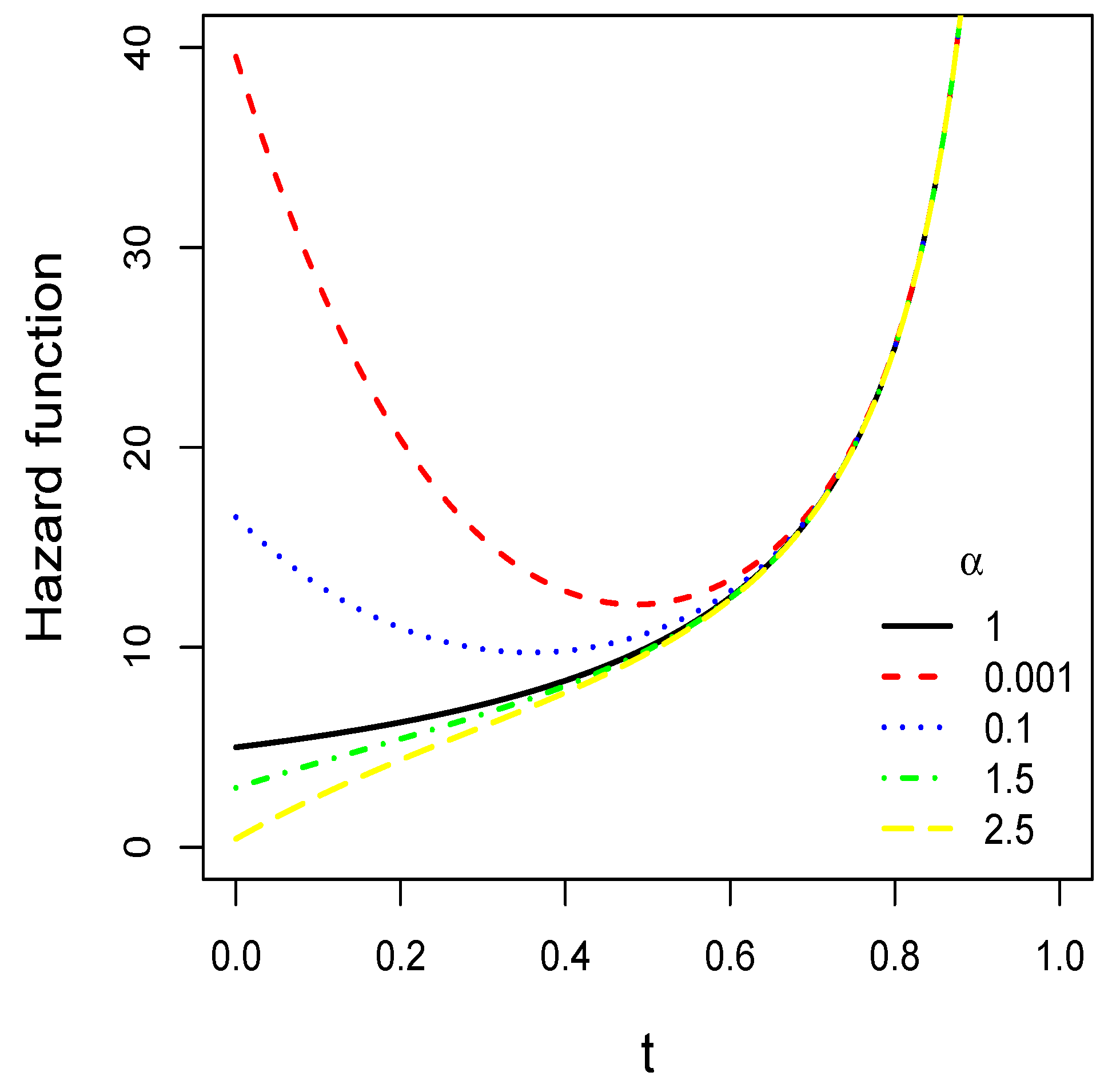
• For $\alpha \ne 1$ and $\beta \ne 1$, we observe that the equation $\partial g(x;\beta ,\alpha )/\partial x=0$ leads to the statement that the LPHU pdf may have a critical point at

  $$\begin{array}{c}\hfill x_0=1-{\left(\frac{3\beta -1-\sqrt{\beta (5\beta -2)+1}}{2\beta log\left(\alpha \right)}\right)}^{\frac{1}{\beta }},\end{array}$$

  where $(x_0,g(x_0;\alpha ,\beta ))$ is a maximum or a minimum if $d\left(x_0\right)<0$ or $d\left(x_0\right)>0$, respectively, such that $d\left(x\right)=-2+\beta (3-\beta )+x_1\{2-\beta (9+7\beta )+\beta x_1[\beta (x_1-6)+3]\}$, where $x_1=log\left(\alpha \right){(1-x)}^{\beta }$.

The upper left panel of Figure 1 shows some LPHU pdf curves for different choices of $\alpha$ and $\beta$. In the figure, it can be seen that the LPHU pdf can present monotonic, unimodal, and reverse-unimodal shapes. In the same figure (upper right panel and lower panels) the histograms of three sets of LPHU pseudo-random numbers are presented together with the B and K pdf’s equipped with the ML estimates. Pseudo-random numbers were generated from Equation (2) by considering a uniform$(0,1)$ random input. In the figure, it can be seen that the B and K pdf’s deviate from the relative frequencies exhibited by the histograms, especially in the lower quantiles, since the B and K pdf’s tend to ∞ or 0 at the lower end of the support. This suggests that the LPHU distribution could have a better performance than the B and K distributions when fitting real data that present a histogram with a behavior similar to that shown in this figure.

R codes for the computation of Equations (3) and (4) and for the generation of pseudo-random numbers from the LPHU distribution are provided in Appendix A.

2.2. Related Distributions

By choosing suitable values for the shapes parameters of the LPHU distribution it is possible to distinguish the following special cases: 1. If $\alpha =1$, the LPHU distribution reduces to the PHU distribution; 2. If $\beta =1$, the LPHU distribution reduces to the LU distribution; 3. If $\alpha =\beta =1$, the LPHU distribution reduces to the U distribution.

It is well known that some distributions such as the exponential, Rayleigh, and power, among others, can be derived as a transformation of a U random variable. Considering these transformations on a LU random variable, we derive the following distributions:

• Let $Y=-\lambda log(1-X)$, where $X\sim \mathrm{LPHU}(\alpha ,\beta =\lambda )$ and $\lambda >0$. Then, Y follows the nonscaled Lambert-exponential distribution. See Iriarte et al. [7];
• Let $Y=\sigma \sqrt{-log(1-X)}$, where $X\sim \mathrm{LPHU}(\alpha ,\beta =1/2)$ and $\sigma >0$. Then, Y follows the Lambert–Rayleigh distribution. See Iriarte et al. [7];
• Let $Y=X^{1/\delta }$, where $X\sim \mathrm{LPHU}(\alpha ,\beta )$ and $\delta >0$. Then, the distribution of Y is a three-parameter distribution that reduces to the K distribution when $\alpha =1$. In this case, the cdf of Y is given by $F(y;\alpha ,\beta ,\delta )=1-{(1-y^{\delta })}^{\beta }{\alpha }^{1-{(1-y^{\delta })}^{\beta }}$, where $y\in [0,1)$. Thus, we refer to this distribution as the Lambert–Kumaraswamy distribution.

Other distributions of the literature can be derived under consideration of appropriate transformations of LPHU random variables. Illustratively, we consider in this section only the three transformations described above. As a final consideration of this section, we highlight that the linear transformation $a+(b-a)X$, where $X\sim \mathrm{LPHU}(\alpha ,\beta )$, with $a<b\in \mathbb{R}$, follows a LPHU distribution on the continuous range $(a,b)$. Therefore, the LPHU distribution can be easily used to fit bounded data to any real range.

2.3. Hazard Rate Function

The reliability function (rf) and the hazard rate function (hrf) play an important role in the analysis of lifetime data in reliability studies. In the following statement the rf and hrf of the LPHU distribution are derived.

Proposition 2.

Let $T\sim \mathrm{LPHU}(\alpha ,\beta )$. Then, the rf and the hrf of T are given by

$$\begin{array}{ccc}\hfill R(t;\alpha ,\beta )& =& {(1-t)}^{\beta }{\alpha }^{1-{(1-t)}^{\beta }}\mathit{and}\hfill \end{array}$$

(5)

$$\begin{array}{ccc}\hfill h(t;\alpha ,\beta )& =& \frac{\beta }{1-t}[1-log\left(\alpha \right){(1-t)}^{\beta }].\hfill \end{array}$$

(6)

Proof. 

If T is a random variable representing the failure time of mechanical units, the rf of T, defined as $R\left(t\right):=\mathbb{P}(T>t)$, $t>0$, indicates the probability that mechanical units survive beyond the time t. If $T\sim \mathrm{LPHU}(\alpha ,\beta )$, the result in (5) is obtained as $P(T>t)=1-P(T\le t)=1-G(t;\alpha ,\beta )$, where $G(·;·,·)$ is as in Equation (3)

On the other hand, the hrf of T, defined as $h\left(t\right):=f\left(t\right)/R\left(t\right)$ (where $f(·)$ is the pdf of T), measures the propensity of a mechanical units to fail or die depending on the age it has reached. If $T\sim \mathrm{LPHU}(\alpha ,\beta )$, the result in (6) is a consequence of Equations (3) and (4).    □

In Proposition 2, it can be seen that the LPHU hrf corresponds to a modification in a multiplicative fashion of the PHU hrf. Furthermore, we observe that

$$\begin{array}{c}\hfill \underset{t\to 1^{-}}{lim}\frac{h(t;\alpha =1,\beta )}{h(t;\alpha ,\beta )}=1,\end{array}$$

which means that the LPHU hft can be understood as a modification in early times of the baseline PHU hrf. Figure 2 shows some LPHU hrf curves considering different choices for $\alpha$ and $\beta$. In the figure, it can be seen that (like the B and K hrf’s) the LPHU hrf can present monotonic and reverse-unimodal shapes.

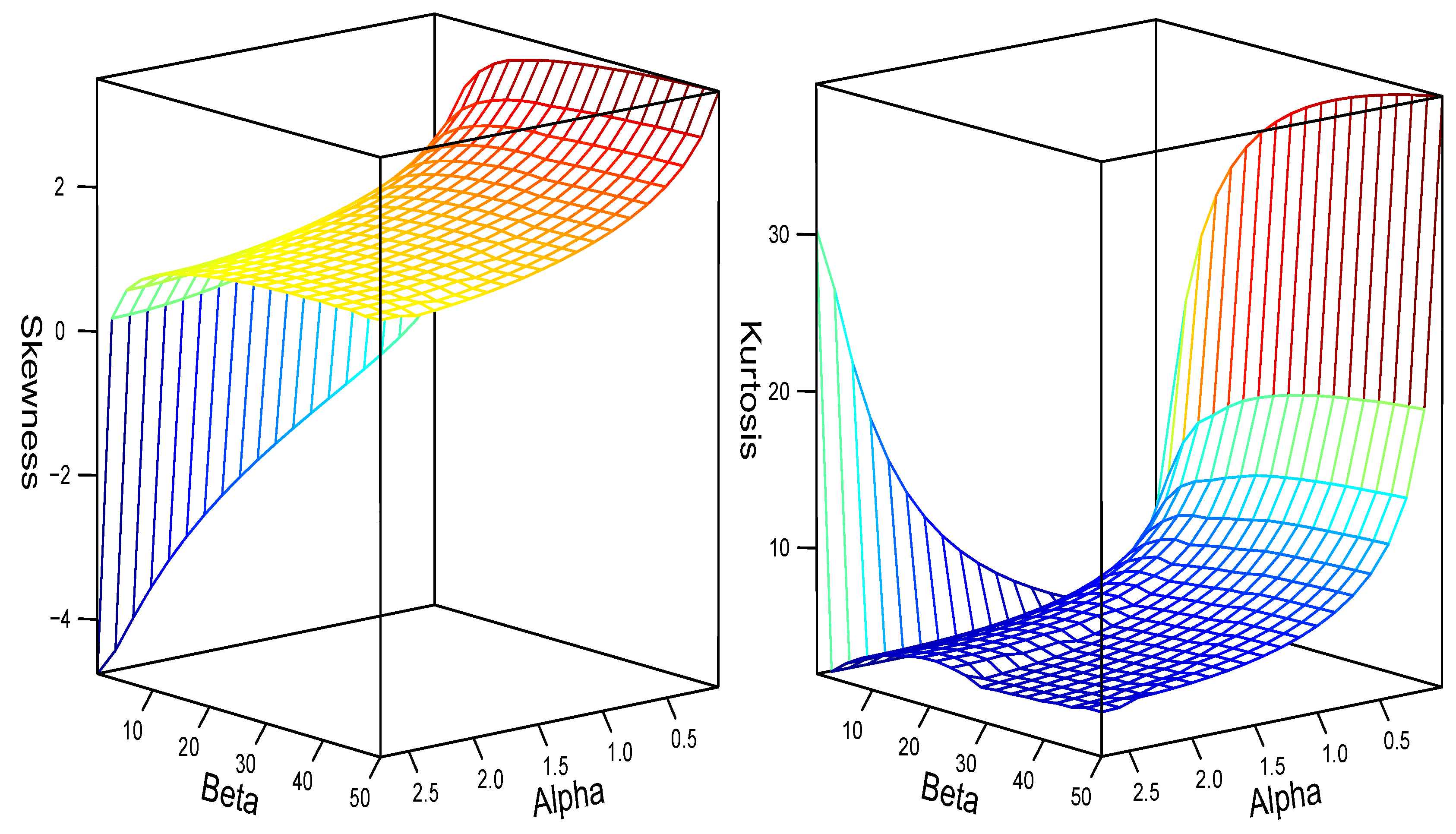
2.4. Skewness and Kurtosis Behavior

In this section, we describe the skewness and kurtosis behavior of the LPHU distribution by analyzing Fisher’s skewness and kurtosis coefficients. For this, we first derive the raw moments.

Proposition 3.

Let $X\sim \mathrm{LPHU}(\alpha ,\beta )$. Then, for $r=1,2,\dots$, the rth raw moment of X is given by

$$\begin{array}{c}\hfill {\mu }_r=\mathbb{E}\left(X^r\right)=1+\alpha \sum _{k=1}^r\left(\genfrac{}{}{0pt}{}{r}{k}\right)a_k(\alpha ,\beta ),\end{array}$$

where $a_k(\alpha ,\beta )={(-1)}^k{\int }_0^1{u}^{k/\beta }{\alpha }^{-u}[1-log\left(\alpha \right)u]du$.

Proof. 

From Equation (4), considering the change of variable $u={(1-x)}^{\beta }$, we obtain that $\mathbb{E}\left(X^r\right)={\int }_0^1{(1-u^{1/\beta })}^r{\alpha }^{1-u}[1-log\left(\alpha \right)u]du$. Thus, the binomial theorem leads to the expression

$$\begin{array}{c}\hfill \mathbb{E}\left(X^r\right)=\alpha \sum _{k=0}^r\left(\genfrac{}{}{0pt}{}{r}{k}\right){(-1)}^k{\int }_0^1{u}^{\frac{k}{\beta }}{\alpha }^{-u}[1-log\left(\alpha \right)u]du,\end{array}$$

and the result is obtained by representing the previous integral as $a_k(\alpha ,\beta )$ and noting that $a_0(\alpha ,\beta )=1/\alpha$.    □

Note that the function $a_k(x;\alpha ,\beta )$ in Proposition 3 must be calculated by numerical integration. A good alternative is to use the integrate function of the R language.

Corollary 2.

Let $X\sim \mathrm{LPHU}(\alpha ,\beta )$. Then, the mean and variance of X are $\mathbb{E}\left(X\right)=1+\alpha a_1$ and $\mathbb{V}\left(X\right)=\alpha (a_2-\alpha a_1^2)$, where $a_j=a_j(\alpha ,\beta )$, with $j=1,2$, is as in Proposition 3.

Corollary 3.

Let $X\sim \mathrm{LPHU}(\alpha ,\beta )$. Then, the Fisher’s skewness and kurtosis coefficients of X are given by

$$\begin{array}{ccc}\hfill \sqrt{{\beta }_1}& =& \frac{\mathbb{E}{[X-\mathbb{E}\left(X\right)]}^3}{{\left[\mathbb{V}\left(X\right)\right]}^{3/2}}=\frac{a_3-3\alpha a_1{a}_2+2{\alpha }^2{a}_1^3}{{\alpha }^{1/2}{(a_2-\alpha a_1^2)}^{3/2}}\mathrm{and}\hfill \\ \hfill {\beta }_2& =& \frac{\mathbb{E}{[X-\mathbb{E}\left(X\right)]}^4}{{\left[\mathbb{V}\left(X\right)\right]}^2}=\frac{a_4-4\alpha a_1{a}_3+6{\alpha }^2{a}_1^2{a}_2-3{\alpha }^3{a}_1^4}{\alpha {(a_2-\alpha a_1^2)}^2},\hfill \end{array}$$

where $a_j=a_j(\alpha ,\beta )$, with $j=1,2,3,4$, is as in Proposition 3.

Due to the analytical complexity it is not possible to obtain closed expressions for the critical points of the Fisher’s skewness and kurtosis coefficients. However, by maximizing and minimizing the coefficients with the help of the R programming language, we obtain approximate ranges of skewness and kurtosis, thus obtaining $\sqrt{{\beta }_1}<4.418$ and ${\beta }_2\in (1.717,46.855)$.

Figure 3 shows the behavior of Fisher’s skewness and kurtosis coefficients for the LPHU distribution. In the figure, it can be seen that the skewness coefficient behaves monotonically with respect to both parameters, a fact that can be understood as an identifiability indicator in the sense that different values of the parameters lead to different skewness levels and, consequently, to different members of the LPHU family. On the other hand, we observe that the kurtosis coefficient can have a non-monotonic behavior, so that there can be two values of $\alpha$ (or $\beta$) associated with the same kurtosis level. This can be understood as the kurtosis levels associated with the weight of the left tail when the distribution is negatively skewed and with the weight of the right tail when it is positively skewed.

3. Parameter Estimation

In this section, we discuss the parameter estimation for the LPHU distribution via the maximum likelihood (ML) method and develop a simulation study to evaluate the behavior of the estimators.

3.1. ML Estimation

Given an observed sample $x_1,\dots ,x_n$ from the random variable $X\sim \mathrm{LPHU}(\alpha ,\beta )$, the log-likelihood function is given by

$$\begin{array}{ccc}\hfill \ell (\alpha ,\beta ;x_i)& =& c(\alpha ,\beta )+(\beta -1)\sum _{i=1}^{n}log\left(z_i\right)-log\left(\alpha \right)\sum _{i=1}^n{z}_i^{\beta }+\sum _{i=1}^{n}log[1-log\left(\alpha \right)z_i^{\beta }],\hfill \end{array}$$

(7)

where $z_i=1-x_i$ and $c(\alpha ,\beta )=nlog\left(\beta \right)+nlog\left(\alpha \right)$.

The ML estimators ${\widehat{\alpha }}_{ML}$ and ${\widehat{\beta }}_{ML}$ of $\alpha$ and $\beta$ can be obtained by taking the partial derivatives of Equation (7) and solving the corresponding system of equations, which is given by the equations

$$\begin{array}{ccc}\hfill n& =& \sum _{i=1}^n{z}_i^{\beta }+\sum _{i=1}^n\frac{z_i^{\beta }}{1-log\left(\alpha \right)z_i^{\beta }}\mathrm{and}\hfill \end{array}$$

(8)

$$\begin{array}{ccc}\hfill \frac{n}{\beta }& =& log\left(\alpha \right)\sum _{i=1}^n{z}_i^{\beta }log\left(z_i\right)-\sum _{i=1}^{n}log\left(z_i\right)+log\left(\alpha \right)\sum _{i=1}^n\frac{z_i^{\beta }log\left(z_i\right)}{1-log\left(\alpha \right)z_i^{\beta }}.\hfill \end{array}$$

(9)

The asymptotic distribution (under regularity conditions) of the ML estimator of $\theta ={(\alpha ,\beta )}^{\prime }$ is $N_2(\theta ,I{(\theta )}^{-1})$, where $I{\left(\theta \right)}^{-1}$ is the expected information matrix. Taking into account the structure of Equation (7), we observe that it is not easy to derive the analytical expression of this matrix. Thus, we consider an approximation from the observed information matrix, where the elements of this matrix are computed as minus the second partial derivatives of the log-likelihood function with respect to each parameter (assessed in the ML estimates).

The observed information matrix is given by

$$\begin{array}{ccc}\hfill I\left(\theta \right)& =& \left(\begin{array}{cc}{\ell }_{\alpha \alpha }& {\ell }_{\alpha \beta }\\ {\ell }_{\alpha \beta }& {\ell }_{\beta \beta }\end{array}\right),\hfill \end{array}$$

where

$$\begin{array}{ccc}\hfill {\ell }_{\alpha \alpha }& =& \frac{n}{{\alpha }^2}-\frac{1}{{\alpha }^2}\sum _{i=1}^n{z}_i^{\beta }-\frac{1}{{\alpha }^2}\sum _{i=1}^n\frac{z_i^{\beta }}{1-log\left(\alpha \right)z_i^{\beta }}+\frac{1}{{\alpha }^2}\sum _{i=1}^n\frac{z_i^{2\beta }}{{[1-log\left(\alpha \right)z_i^{\beta }]}^2},\hfill \\ \hfill {\ell }_{\alpha \beta }& =& \frac{n}{{\beta }^2}+log\left(\alpha \right)\sum _{i=1}^n{z}_i^{\beta }{log}^2\left(z_i\right)+log\left(\alpha \right)\sum _{i=1}^n\frac{z_i^{\beta }{log}^2\left(z_i\right)}{1-log\left(\alpha \right)z_i^{\beta }}+{log}^2\left(\alpha \right)\sum _{i=1}^n\frac{z_i^{2\beta }{log}^2\left(z_i\right)}{{[1-log\left(\alpha \right)z_i^{\beta }]}^2}\hfill \\ & \mathrm{and}& \\ \hfill {\ell }_{\beta \beta }& =& \frac{1}{\alpha }\sum _{i=1}^n{z}_i^{\beta }log\left(z_i\right)+\frac{1}{\alpha }\sum _{i=1}^n\frac{z_i^{\beta }log\left(z_i\right)}{1-log\left(\alpha \right)z_i^{\beta }}+\frac{log\left(\alpha \right)}{\alpha }\sum _{i=1}^n\frac{z_i^{2\beta }log\left(z_i\right)}{{[1-log\left(\alpha \right)z_i^{\beta }]}^2}.\hfill \end{array}$$

Then, approximate $100(1-\phi )$% confidence intervals for $\alpha$ and $\beta$ can be determined by $\widehat{\alpha }\pm z_{\phi /2}{s}_{\widehat{\alpha }}$ and $\widehat{\beta }\pm z_{\phi /2}{s}_{\widehat{\beta }}$, respectively, where $z_{\phi /2}$ is the upper $(\phi /2)$th percentile of the standard normal distribution, and $s_{\widehat{\alpha }}$ and $s_{\widehat{\beta }}$ are the diagonal elements of the matrix ${\left[I\left(\theta \right)\right]}^{-1}$ (assessed in the ML estimates).

3.2. Computational Guidelines

From Equations (8) and (9), it can be seen that the ML estimators cannot be obtained explicitly, so the estimates must be obtained using numerical procedures. A good alternative for this is to use the multiroot function [14] of the R programming language, which implements the Newton–Raphson method for obtaining roots of systems of nonlinear equations.

Due to the above, we consider the following points:

• Alternatively, the ML estimates can be obtained by solving the optimization problem ${max}_{(\alpha ,\beta )}{\sum }_{i=1}^n\ell (\alpha ,\beta ;x_i)$, subject to $\alpha \in (0,e)$, $\beta >0$, where $\ell (·;·)$ is given in Equation (7).
• For this, we use the optim function of the R programming language. An R code is provided in Appendix B.
• Specifically, we consider the L-BGSB-B algorithm [15], which allows us to specify the parameter space. This algorithm requires declaring a value in the parameter space to initialize the iterative process. Taking into account that the PHU distribution is a special case of the LPHU distribution, we consider ${\alpha }_0=1$ and ${\beta }_0=-n/{\sum }_{i=1}^{n}log(1-x_i)$, where ${\beta }_0$ is the ML estimator of the shape parameter of the PHU distribution.

3.3. Simulation Study

We generate 1000 random samples from the LPHU distribution under the sample sizes $n=10$, 20, 30, …, 1500, respectively, and consider the following scenarios: Scenario A, where $\alpha =1.5$ and $\beta =2.0$, being the pseudo-random numbers generated from a unimodal LPHU distribution; Scenario B, where $\alpha =0.5$ and $\beta =0.6$, being the pseudo-random numbers generated from a LPHU distribution with reverse-unimodal pdf; Scenario C, where $\alpha =2.0$ and $\beta =0.7$, being th pseudo-random numbers generated from a LPHU distribution with increasing pdf.

Pseudo-random numbers were generated from Equation (2) considering the following steps:

• Generate $u\sim \mathrm{uniform}(0,1)$;
• Compute $x=1-{\left[-\frac{1}{log\left(\alpha \right)}{W}_0\left(\frac{log\left(\alpha \right)(u-1)}{\alpha }\right)\right]}^{\frac{1}{\beta }}$.

For each simulated sample, we obtain the ML estimate following the guidelines of Section 3.1. The R code used in scenario A is provided in Appendix C. For scenarios B and C it is enough to modify the initial parameters.

Figure 4, Figure 5 and Figure 6 illustrate the behavior of the average estimate (AE), the standard deviation (SD), the square root of the simulated mean square error (RMSE), the average of the asymptotic standard error (SE), and the probability of coverage of the 95% asymptotic confidence interval (CP) for each set of 1000 estimates obtained under the different sample sizes and scenarios considered. Looking at the figures, we can see that the AE’s tend to be close to the true values of the parameters as the sample size increases. An overestimation of the parameters is observed when the estimates are obtained from small samples ($n=10$), which decreases rapidly as the sample size increases. The SD’s, RMSE’s, and SE’s are close and decrease towards 0 as the sample size increases, as expected in the standard asymptotic theory. Similarly, the CP’s converge to the nominal values used to construct the confidence intervals as the sample size increases.

4. Data Analysis

In this section, we present two applications of the LPHU distribution in which its performance in fitting real data is contrasted with that of the B and K distributions.

4.1. Firm’s Risk Management Cost Effectiveness

We consider 73 observations on the measure of the firm’s risk management cost effectiveness presented by Schmit and Roth [16]. Some descriptive statistics of the data are as follows: Minimum, 0.0020; Maximum, 0.9755; Fisher’s skewness coefficient, 3.7154; Fisher’s kurtosis coefficient, 17.957.

Table 1. The parameter estimates with standard errors in parentheses, the AIC and BIC values, and the p-values of the AD and CvM goodness-of-fit tests for each distribution fitted to the firm’s risk management cost effectiveness data.

Distribution	$\widehat{\mathit{\alpha }}$	$\widehat{\mathit{\beta }}$	AIC	BIC	AD	CvM
LPHU	0.012	1.889	−174.3	−169.7	0.484	0.616
	(0.016)	(0.496)
K	0.664	3.440	−153.3	−148.7	0.025	0.039
	(0.071)	(0.620)
B	0.612	3.797	−148.2	−143.7	0.009	0.013
	(0.085)	(0.715)

reports the ML estimates, the values associated with the Akaike Information Criterion (AIC) [17], and the Bayesian Information Criterion (BIC) [18], and the p-values of the traditional Anderson–Darling (AD) and Cramer–von Mises (CvM) goodness of fit tests [19] for the LPHU, B, and K distributions fitted to the firm’s risk management cost effectiveness data. Looking at the table, under the 0.05 significance level, we note that the p-values indicate that only the LPHU distribution appropriately models the firm’s risk management cost effectiveness data. In addition, it can be seen that the LPHU distribution is the one with the lowest AIC and BIC values among the fitted distributions, suggesting that this distribution should be selected for modeling the firm’s risk management cost effectiveness data.

We observe that the LPHU pdf, equipped with the ML estimates provided in Table 1, takes the value $\widehat{\beta }(1-log\left(\widehat{\alpha }\right))=$ 2.846 at the lower end of its support, allowing for more accurate modeling of the lower empirical quantiles. Figure 7 presents the empirical distribution contrasted with the fitted LPHU, B, and K distributions. In the Figure, it can be seen that the lower empirical quantiles are closer to the LPHU distribution quantiles.

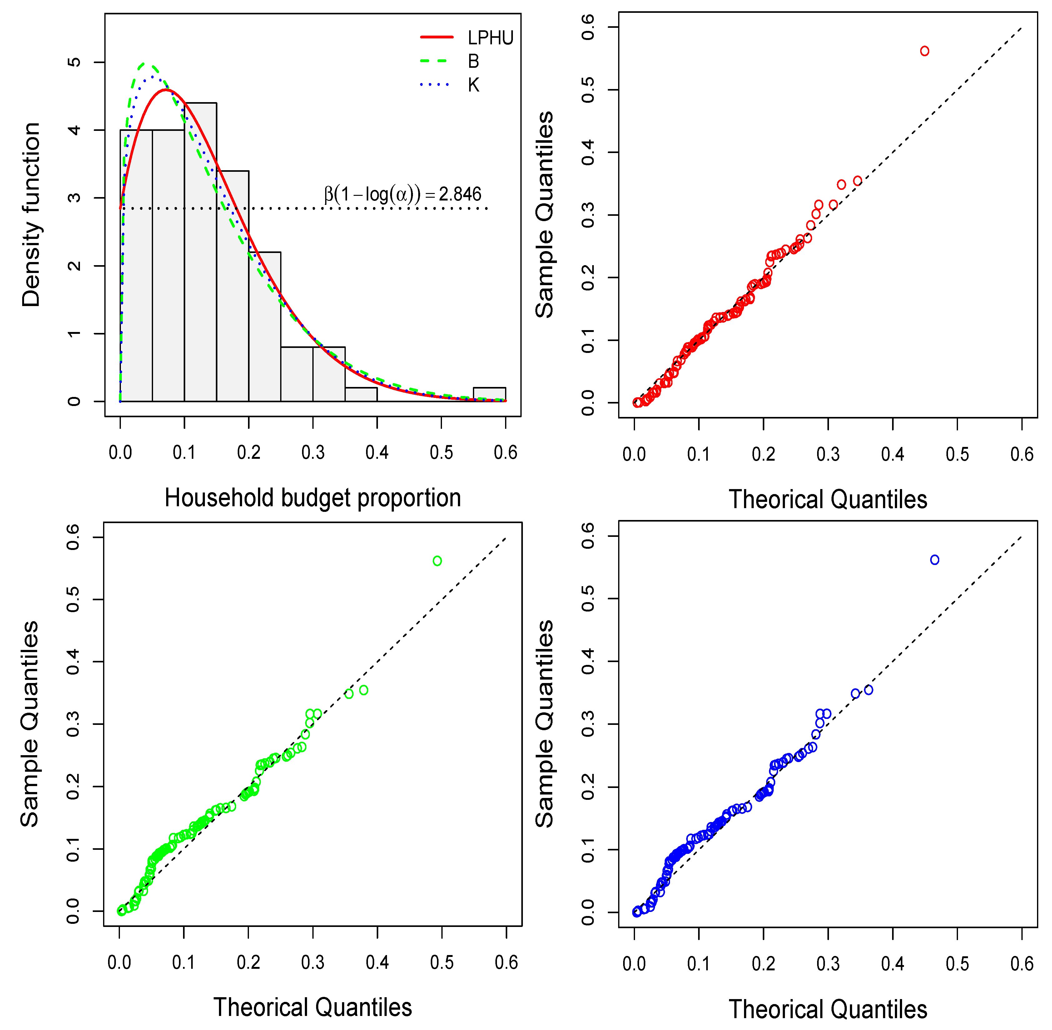
4.2. Household Shared Budget for Transportation

Studies on the shared household budget are highly valued when trying to find out the evolution of the price level faced by households in a given locality, see for example Blundell et al. [3]. The BudgetUk database [20] of the R language provides information on the proportion of the shared budget that British households spend on different items such as food, clothing, transport, fuel, and alcohol.

In this application, we compare the performance of the LPHU, B, and K distributions by modeling the proportion of the shared budget of households that allocate part of the budget to transportation. These data correspond to 1473 observations bounded to the interval $(0,1)$ whose histogram exhibits a unimodal behavior. From now on, we will refer to these data simply as the household shared budget proportion data.

For comparison, we use the sample function of the R language to obtain 1000 random samples of size 100 from the household shared budget proportion data. Based on the modified AD and CvM goodness-of-fit tests [21], under the 0.05 significance level, we calculate the proportion of samples where the LPHU, B, and K distributions fit the data appropriately. We call this the non-rejection rate. Additionally, we calculate the proportion of samples where each distribution presents the lowest AIC and BIC values, that is, the proportion of samples where each distribution exhibits the best performance. We call this the hit rate.

Table 2. Non-rejection rates based on modified AD ($A^{*}$) and CvM ($W^{*}$) statistics and hit rates based on AIC and BIC values for the LPHU, B, and K distributions fitted to the 1000 samples obtained from the household shared budget proportion data.

	Non-Rejection Rate		Hit Rate
Distribution	${\mathit{w}}^{*}$	${\mathit{A}}^{*}$	AIC	BIC
LPHU	0.734	0.718	0.836	0.836
B	0.502	0.479	0.130	0.130
K	0.562	0.531	0.034	0.034

reports the values associated with the non-rejection and hit rates for the LPHU, B, and K distributions fitted to the 1000 samples. In the table, we observe that the LPHU distribution is able to adequately fit a larger proportion of samples than the B and K distributions. In addition, we see that the performance of the LPHU distribution is better in a large proportion of samples, in 83.6% of the samples.

Table 3. ML estimates (with SE in parentheses), AIC and BIC values, and modified AD ($W^{*}$) and CvM ($A^{*}$) statistics for the LPHU, B, and K distributions fitted to a single sample obtained from the household shared budget proportion data.

Distribution	$\widehat{\mathit{\alpha }}$	$\widehat{\mathit{\beta }}$	AIC	BIC	${\mathit{W}}^{*}$	${\mathit{A}}^{*}$
LPHU	1.996	9.222	−209.5	−204.3	0.112	0.715
	(0.259)	(0.933)
B	1.302	8.217	−203.1	−197.8	0.213	1.308
	(0.166)	(1.228)
K	1.273	10.539	−105.1	−199.9	0.177	1.092
	(0.116)	(2.385)

shows the parameter estimates and the AIC, BIC, $W^{*}$ and $A^{*}$ values for the LPHU, B, and K distributions fitted to a single sample obtained from the household shared budget proportion data. Looking at the table, it can be seen that the LPHU distribution performs more accurately than the B and K distributions. We note that the fitted LPHU pdf takes the value $\widehat{\beta }(1-log\left(\widehat{\alpha }\right))=$ 2.846 at the lower end of its support. This allows the LPHU distribution to more appropriately fit the lower empirical quantiles than the B and K distributions. This is illustrated in the upper left panel of Figure 8. In the upper right panel and the lower panels of Figure 8, the qq-plots for the LPHU, B and K distributions are presented, where it can be seen that the LPHU distribution presents a better fit of the lower quantiles.

5. Concluding Remarks

We propose a new two-parameter distribution for the fit of bounded data. The pdf of the new distribution, called the LPHU distribution, presents shapes similar to those exhibited by the popular B and K distributions, but with the characteristic that it tends towards a positive finite value at the lower end of its support. The latter may lead to a better fit of the lower empirical quantiles of certain datasets. Structural properties such as pdf, cdf, and hrf have a closed analytical structure, so they are easy to process computationally. From the description of Fisher’s skewness and kurtosis coefficients for the LPHU distribution, it is concluded that the LPHU distribution can present both positive and negative skewness, and is also capable of capturing high levels of kurtosis. Regarding the parameter estimation, the ML estimators for the LPHU distribution do not have a closed form, so it is necessary to use numerical procedures to obtain the estimates. We use the optim function of the R programming language to accomplish this task. Simulation studies show that the ML method provides acceptable estimates for the parameters of the LPHU distribution. Finally, two application examples illustrate that the LPHU distribution can perform better when fitting real data than the popular B and K distributions.

References

1. Johnson, N.L.; Kotz, S.; Balakrishnan, N. Continuous Univariate Distributions; John Wiley & Sons: Hoboken, NJ, USA, 1995; Volume 2. [Google Scholar]
2. Kumaraswamy, P. A generalized probability density function for double-bounded random processes. J. Hydrol. 1980, 46, 79–88. [Google Scholar] [CrossRef]
3. Blundell, R.; Duncan, A.; Pendakur, K. Semiparametric estimation and consumer demand. J. Appl. Econom. 1998, 13, 435–461. [Google Scholar] [CrossRef]
4. Dey, S.; Mazucheli, J.; Nadarajah, S. Kumaraswamy distribution: Different methods of estimation. Comput. Appl. Math. 2018, 37, 2094–2111. [Google Scholar] [CrossRef]
5. Wang, J.Z. A note on estimation in the four-parameter beta distribution. Commun.-Stat.-Simul. Comput. 2005, 34, 495–501. [Google Scholar] [CrossRef]
6. Smith, R.L. Maximum likelihood estimation in a class of nonregular cases. Biometrika 1985, 72, 67–90. [Google Scholar] [CrossRef]
7. Iriarte, Y.A.; de Castro, M.; Gómez, H.W. The Lambert-F distributions class: An alternative family for positive data analysis. Mathematics 2020, 8, 1398. [Google Scholar] [CrossRef]
8. Corless, R.M.; Gonnet, G.H.; Hare, D.E.; Jeffrey, D.J.; Knuth, D.E. On the LambertW function. Adv. Comput. Math. 1996, 5, 329–359. [Google Scholar] [CrossRef]
9. Brito, P.; Fabiao, F.; Staubyn, A. Euler, Lambert, and the Lambert W function today. Math. Sci. 2008, 33. [Google Scholar]
10. Iriarte, Y.A.; de Castro, M.; Gómez, H.W. An alternative one-parameter distribution for bounded data modeling generated from the Lambert transformation. Symmetry 2021, 13, 1190. [Google Scholar] [CrossRef]
11. Martínez-Florez, G.; Moreno-Arenas, G.; Vergara-Cardozo, S. Properties and inference for proportional hazard models. Rev. Colomb. Estad. 2013, 36, 95–114. [Google Scholar]
12. Adler, A. lamW: Lambert-W Function. 2015. R Package Version 2.1.1. Available online: https://doi.org/10.5281/zenodo.5874874 (accessed on 5 January 2023).
13. R Core Team. R: A Language and Environment for Statistical Computing; R Foundation for Statistical Computing: Vienna, Austria, 2021. [Google Scholar]
14. Soetaert, K. rootSolve: Nonlinear Root Finding, Equilibrium and Steady-State Analysis of Ordinary Differential Equations. 2009. R Package Version 1.6. Available online: https://CRAN.R-project.org/package=rootSolve (accessed on 5 January 2023).
15. Byrd, R.H.; Lu, P.; Nocedal, J.; Zhu, C. A limited memory algorithm for bound constrained optimization. SIAM J. Sci. Comput. 1995, 16, 1190–1208. [Google Scholar] [CrossRef]
16. Schmit, J.T.; Roth, K. Cost effectiveness of risk management practices. J. Risk Insur. 1990, 57, 455–470. [Google Scholar] [CrossRef]
17. Akaike, H. A new look at the statistical model identification. IEEE Trans. Autom. Control. 1974, 19, 716–723. [Google Scholar] [CrossRef]
18. Schwarz, G. Estimating the dimension of a model. Ann. Stat. 1978, 6, 461–464. [Google Scholar] [CrossRef]
19. Faraway, J.; Marsaglia, G.; Marsaglia, J.; Baddeley, A. Goftest: Classical Goodness-of-Fit Tests for Univariate Distributions. R Package Version 1.2-3. 2021. Available online: https://CRAN.R-project.org/package=goftest (accessed on 5 January 2023).
20. Croissant, Y.; Graves, S. Ecdat: Data Sets for Econometrics. R Package Version 0.4-2. 2022. Available online: https://CRAN.R-project.org/package=Ecdat (accessed on 5 January 2023).
21. Chen, G.; Balakrishnan, N. A general purpose approximate goodness-of-fit test. J. Qual. Technol. 1995, 27, 154–161. [Google Scholar] [CrossRef]
Figure 1. Top left: Some LPHU pdf curves considering different values for α and β . Top right and bottom: Histograms for three sets of 1000 pseudorandom numbers from the LPHU distribution, with ( α , β ) = (1.7, 2), (0.5, 1.5), and (0.2, 0.5), respectively, fitted with the B and K distributions via the ML method.
Mathematics 11 00667 g001
Figure 2. Some LPHU hrf curves for β = 5 and different values of α .
Mathematics 11 00667 g002
Figure 3. Fisher’s skewness and kurtosis coefficients for the LPHU distribution.
Mathematics 11 00667 g003
Figure 4. The AE, SD, RMSE, SE, and CP for each of the 1000 estimates of α (top) and β (bottom) obtained in scenario A, under the different sample sizes.
Mathematics 11 00667 g004
Figure 5. The AE, SD, RMSE, SE, and CP for each of the 1000 estimates of α (top) and β (bottom) obtained in scenario B, under the different sample sizes.
Mathematics 11 00667 g005
Figure 6. The AE, SD, RMSE, SE, and CP for each of the 1000 estimates of α (top) and β (bottom) obtained in scenario C, under the different sample sizes.
Mathematics 11 00667 g006
Figure 7. (Left): Histogram for the firm’s risk management cost effectiveness data and the fitted pdf curves via the ML method. (Right): Empirical cdf for the firm’s risk management cost effectiveness data and the fitted cdf curves.
Mathematics 11 00667 g007
Figure 8. Top left: Histogram for a single sample obtained from the household shared budget proportion data and the fitted pdf curves via the ML method. Top right and lower: QQ-plots for the LPHU (red), B (green), and K (blue) distributions.
Mathematics 11 00667 g008