Computational Analysis of the Fractional Riccati Differential Equation with Prabhakar-type Memory

Abstract

The key objective of the current work is to examine the behavior of the nonlinear fractional Riccati differential equation associated with the Caputo–Prabhakar derivative. An efficient computational scheme, that is, a mixture of homotopy analysis technique and sumudu transform, is used to solve the nonlinear fractional Riccati differential equation. The convergence and uniqueness analysis for the solution of the implemented technique is shown. In addition, the numerical consequences are demonstrated in the form of graphical representations to verify the reliability of the applied method in obtaining the solution to the mathematical model with Prabhakar-type memory.

1. Introduction

A special branch of mathematical sciences, which involves the study and applications of integrals and derivatives of arbitrary order, is known as fractional calculus (FC); moreover, we can say that it generalizes the concept of an integer order derivative to an arbitrary order derivative. The idea of FC is not new; however, in the last three decades, many researchers and mathematicians have shown interest in the study of FC because of its applications in almost every field of real life. FC provides a remarkable contribution to mathematical modeling by converting physical problems into mathematical models and giving approximate and efficient solutions to the problems [1,2,3,4]. Mathematicians and researchers have developed many fractional derivatives, including the Riemann–Liouville derivative, the Grünwald–Letnikov derivative, the Caputo derivative of arbitrary order, etc. To describe some real-world problems, one can use other derivatives of arbitrary order, for example, the Prabhakar, Caputo–Prabhakar, Hilfer–Prabhakar, and many other derivatives [5,6,7].

In this work, we consider the Riccati differential equation, named after the Italian nobleman Count Jacopo Francesco Riccati (1676–1754), in the form

$$C_1\left(t\right)\frac{du\left(t\right)}{dt}+C_2\left(t\right)u\left(t\right)+C_3\left(t\right)u^2\left(t\right)=\psi \left(t\right),a\le t\le b,$$

(1)

with initial guess $u\left(0\right)=c$, where $C_1\left(t\right),C_2\left(t\right),C_3\left(t\right)$, and $\psi \left(t\right)$ are continuous and real-valued functions. The Riccati differential equation has many applications in the field of applied sciences, engineering, and real-world problems, such as pattern formation in dynamic gases, control theory, diffusion problems, network synthesis, river flows, invariant embedding, and econometric models. Hence, to produce more efficient and approximate results, many studies have been conducted, with many analytical and numerical methods emerging. These include a new homotopy perturbation technique proposed by Khan et al. [8]; the modified variation iteration method (MVIM) applied by Geng [9]; and a fractional variational iteration approach employed by Merdan [10] to determine the solution to the Riccati differential equation of arbitrary order. In addition, Sakar et al. [11] presented an iterative reproducing kernel Hilbert space technique to study the Riccati differential equation of non-integer order; Ghomanjani et al. [12] presented the approximate solution of the quadratic Riccati differential equation by employing the Bezier curves technique; Eldien et al. [13] used the concept of the Chebyshev polynomial to obtain the solution of the Riccati differential equation; Rasdee et al. [14] introduced a three point clock multistep technique in backward difference form; Ranjbar et al. [15] implemented an enhanced homotopy perturbation technique; Liu et al. [16] employed a technique based on the quadrature rule and Laplace transform; and Tan et al. [17] used the homotopy analysis approach to determine the solution to the Riccati differential equation of quadratic type.

In this work, we apply an efficient analytical method associated with sumudu transform (ST) and the homotopy analysis technique, namely the homotopy analysis sumudu transform method (HASTM) [18] to determine the approximate analytical solution to the nonlinear fractional Riccati differential (FRD) equation. The FRD equation associated with the Prabhakar derivative in the Caputo sense is given by

$$C_1\left(t\right){}^C{D}_{\alpha ,\mu ,w,0^{+}}^{\lambda }u\left(t\right)+C_2\left(t\right)u\left(t\right)+C_3\left(t\right)u^2\left(t\right)=\psi \left(t\right),$$

(2)

where ${}^C{D}_{\alpha ,\mu ,w,0^{+}}^{\lambda }u\left(t\right)$ narrates the fractional order derivative in the Caputo–Prabhakar sense. For $\mu =1$and$\lambda =0$, Equation (2) reduces to Equation (1).

The reason for using this method is not only that it handles the nonlinear terms very easily by using He’s polynomial but also that it involves an auxiliary parameter ℏ that controls the convergence of obtained HASTM solution. This article is organized as follows: some basic concepts of the Caputo–Prabhakar derivative and ST are described in Section 2. The elementary plan of the applied technique is given in Section 3. The convergence and the uniqueness of the FRD equation is analyzed in Section 4. The solution to some FRD equations using HASTM is given in Section 5. The numerical results, graphical representations, and comparison of the results obtained by the applied technique with previous techniques are presented in Section 6. Section 7 contains some concluding remarks.

2. Some Preliminary Definitions

Here, we discuss some definitions and results related to the fractional operator [19,20,21,22,23,24,25].

Definition 1.

Let $g\left(t\right)\in L^1\left[a,b\right]$, where $-\infty \le a<t<b\le \infty$, be a locally integrable real-valued function; then, the Riemann–Liouville (RL) derivative of arbitrary order μ is presented as [1]

$$D_{a^{+}}^{\mu }g\left(t\right)=\frac{1}{\mathsf{\Gamma }(m-\mu )}\frac{d^m}{{dt}^m}{\int }_a^t{\left(t-\tau \right)}^{m-1-\mu }g\left(\tau \right)d\tau ,$$

(3)

where$m-1<\mu \le m$, and $m\in \mathbb{N}$.

Definition 2.

For $\mu >0$ and $g\in {AC}^m\left[a,b\right]$, the Caputo derivative of arbitrary order μ is given as [1]

$${{}_a^{C}D}_t^{\mu }g\left(t\right)=\frac{1}{\mathsf{\Gamma }(m-\mu )}{\int }_a^t{\left(t-\tau \right)}^{m-1-\mu }\frac{d^m}{{dt}^m}g\left(\tau \right)d\tau .$$

(4)

Here, $m\in \mathbb{N}$, and ${AC}^m\left[a,b\right]$ represents the space of the real-valued function$g\left(t\right)$, which possesses a continuous derivative up to order $m-1$ on $\left[a,b\right]$, such that $g^{m-1}\left(t\right)$ belongs to the space of the absolutely continuous functions $\left[a,b\right]$, defined as follows

$${AC}^m\left[a,b\right]=\left\{g:\left[a,b\right]⟶\mathbb{R}:\frac{d^{m-1}}{{dt}^{m-1}}g\left(t\right)\in AC\left[a,b\right]\right\}.$$

(5)

Definition 3.

The Indian mathematician T.L. Prabhakar introduced a three-parameter Mittag–Leffler function known as the Prabhakar function, which is defined as [19,21]

$$E_{\alpha ,\mu }^{\lambda }\left(t\right)=\sum _{k=0}^{\infty }\frac{{\left(\lambda \right)}_k}{\mathsf{\Gamma }\left(\alpha k+\mu \right)}\frac{t^k}{k!},$$

(6)

where$\alpha ,\mu ,\lambda \in \mathbb{C},\mathfrak{R}\left(\alpha \right)>0$, and ${\left(\lambda \right)}_k$ denotes the Pochhammer symbol.

Definition 4.

Suppose that $g\left(t\right)\in L^1\left[a,b\right]$, where $-\infty \le a<t<b\le \infty$; then, the Prabhakar integral is given as [19,21,22]

$${\mathbb{E}}_{\alpha ,\mu ,w,a^{+}}^{\lambda }g\left(t\right)={\int }_a^t{\left(t-\tau \right)}^{\mu -1}{E}_{\alpha ,\mu }^{\lambda }\left(w{\left(t-\tau \right)}^{\alpha }\right)g\left(\tau \right)d\tau ,$$

$$=\left(e_{\alpha ,\mu }^{\lambda }(•;w)\ast g\right),$$

(7)

i.e., we can say that the Prabhakar integral is a convolution of functions $g\left(t\right)$ and $e_{\alpha ,\mu }^{\lambda }(t;w)$, where $e_{\alpha ,\mu }^{\lambda }(t;w)=t^{\mu -1}{E}_{\alpha ,\mu }^{\lambda }\left(w{t}^{\alpha }\right)$ for $\alpha ,\mu ,w,\lambda \in \mathbb{C}$, with $\mathfrak{R}\left(\alpha \right),\mathfrak{R}\left(\mu \right)>0$.

Definition 5.

Let$g\in L^1\left[a,b\right]$, $-\infty \le a<t<b\le \infty$, and$\left(e_{\alpha ,\mu }^{\lambda }(•;w)\ast g\right)\in W^{m,1}\left(a,b\right)$; then, the Prabhakar derivative in the RL sense is defined as [21,23]

$${\mathbb{D}}_{\alpha ,\mu ,w,a^{+}}^{\lambda }g\left(t\right)=\frac{d^m}{{dt}^m}{\mathbb{E}}_{\alpha ,m-\mu ,w,a^{+}}^{-\lambda }g\left(t\right),$$

(8)

where $\mu ,w,\lambda ,\alpha \in \mathbb{C},\mathfrak{R}\left(\alpha \right),\mathfrak{R}\left(\mu \right)>0,m-1<\mu \le m,m\in \mathbb{N}$, and $W^{m,1}\left[a,b\right]$ is the Sobolev space given as

$$W^{m,1}\left[a,b\right]=\left\{g\in L^1\left[a,b\right]:\frac{d^m}{{dt}^m}g\in L^1\left[a,b\right]\right\}.$$

(9)

Definition 6.

Let $g\in {AC}^m\left[a,b\right],0\le a<t<b\le \infty$, and $\alpha ,\mu ,w,\lambda \in \mathbb{C}$, with $\mathfrak{R}\left(\alpha \right),\mathfrak{R}\left(\mu \right)>0$. Then the Caputo–Prabhakar derivative of arbitrary order μ is given as [20,21,23,24]

$${}^C{\mathbb{D}}_{\alpha ,\mu ,w,a^{+}}^{\lambda }g\left(t\right)={\int }_a^t{\left(t-\tau \right)}^{m-\mu -1}{E}_{\alpha ,m-\mu }^{-\lambda }\left(w{\left(t-\tau \right)}^{\alpha }\right)g^{\left(m\right)}\left(\tau \right)d\tau ,$$

(10)

$$={\mathbb{E}}_{\alpha ,m-\mu ,w,a^{+}}^{-\lambda }\frac{d^m}{{dt}^m}g\left(t\right),m-1<\mu \le m.$$

(11)

It is also known as the regularized Prabhakar derivative. For $\lambda =0$, the Caputo–Prabhakar derivative becomes the Caputo derivative [21] as $E_{\alpha ,\mu }^0\left(t\right)=\frac{1}{\mathsf{\Gamma }\left(\mu \right)}$.

Definition 7.

Consider a set of functions B defined as

$$B=\left\{g\left(t\right):\exists C,{\eta }_1,{\eta }_2>0,\left|g\left(t\right)\right|<C{e}^{\left|t\right|/{\eta }_j},ift\in {\left(-1\right)}^j\times [0,\infty )\right\}.$$

(12)

Watugala [26] defined ST over the set of functions B, as

$$S\left[g\left(t\right)\right]\left(s\right)=G\left(s\right)={\int }_0^{\infty }\frac{1}{s}{e}^{-t/s}g\left(t\right)dt,s\in \left(-{\eta }_1,{\eta }_2\right).$$

(13)

The detailed properties of the ST can be found in [27,28]. The ST of the Caputo–Prabhakar derivative [29] is

$$S\left[{{}^C\mathbb{D}}_{\alpha ,\mu ,w,a^{+}}^{\lambda }g\left(t\right)\right]\left(s\right)=s^{-\mu }{\left(1-w{s}^{\alpha }\right)}^{\lambda }\left[G\left(s\right)-g\left(a^{+}\right)\right].$$

(14)

3. Fundamental Description of HASTM

To give a fundamental description of the applied analytical technique, we assume a nonlinear differential equation of fractional order

$${}^C{D}_{\alpha ,\mu ,w,0^{+}}^{\lambda }u\left(t\right)+Ru\left(t\right)+Nu\left(t\right)=\psi \left(t\right),m-1<\mu \le m,m\in \mathbb{N},$$

(15)

where $u\left(t\right)$ is a function of t, ${}^C{D}_{\alpha ,\mu ,w,0^{+}}^{\lambda }$ represents the Caputo–Prabhakar derivative of arbitrary order $\mu$, $m\in \mathbb{N},R$ is the bounded linear operator of t, the general nonlinear operator is represented by N, which is Lipschitz continuous, and $\psi \left(t\right)$ is a source term.

Implementing the ST operator on Equation (15), we obtain

$$S\left[{}^C{D}_{\alpha ,\mu ,w,0^{+}}^{\lambda }u\right]+S\left[Ru+Nu\right]=S\left[\psi \left(t\right)\right].$$

(16)

On using the differentiation properties of the ST, we obtain the following equation

$$s^{-\mu }{\left(1-w{s}^{\alpha }\right)}^{\lambda }S\left[u\right]-s^{-\mu }{\left(1-w{s}^{\alpha }\right)}^{\lambda }u\left(0\right)+S\left[Ru+Nu\right]=S\left[\psi \left(t\right)\right].$$

(17)

On simplifying Equation (17), we obtain the subsequent equation

$$S\left[u\right]-u\left(0\right)+s^{\mu }{\left(1-w{s}^{\alpha }\right)}^{-\lambda }\left[S\left[Ru+Nu\right]-S\left[\psi \left(t\right)\right]\right]=0.$$

(18)

According to Equation (18), the nonlinear operator is given as

$$N\left[\zeta \left(t;q\right)\right]=S\left[\zeta \left(t;q\right)\right]-\zeta \left(t;q\right)\left(0\right)$$

$$+s^{\mu }{\left(1-w{s}^{\alpha }\right)}^{-\lambda }\left[S\left[R\zeta \left(t;q\right)+N\zeta \left(t;q\right)\right]-S\left[\psi \left(t\right)\right]\right],$$

(19)

where $\zeta (t;q)$ represents a function of t and q, q is an embedding parameter such that $0\le q\le 1$, and the homotopy can be written as

$$\left(1-q\right)S\left[\zeta \left(t;q\right)-u_0\right]=\hslash N\left[u\left(t\right)\right],$$

(20)

where$S$ represents the ST operator, $u_0\left(t\right)$ is an initial approximation of $u\left(t\right)$, $\zeta (t;q)$ is an unknown function, and ℏ is a nonzero auxiliary parameter. Moreover, it may be clarified that, by substituting the values of the embedding parameter $q=0$ as well as $q=1$, it gives

$$\zeta \left(t;0\right)=u_0\left(t\right),\zeta \left(t;1\right)=u\left(t\right),$$

(21)

appropriately. So, we can say that as q varies from 0 to 1, the solution of $\zeta \left(t;q\right)$ varies from the initial approximation $u_0\left(t\right)$ to the solution$u\left(t\right)$. The Taylor’s series expansion of the function $\zeta \left(t;q\right)$ is given as follows

$$\zeta \left(t;q\right)=u_0\left(t\right)+\sum _{k=1}^{\infty }{u}_k\left(t\right)q^k,$$

(22)

where

$$u_k\left(t\right)=\frac{1}{k!}\frac{{\partial }^k}{{\partial q}^k}{\left\{\zeta \left(t;q\right)\right\}|}_{q=0}.$$

(23)

If the initial guess $u_0\left(t\right)$ and the convergence control parameter ℏ are described appropriately, then Equation (22) converges at $q=1$; then, we obtain the subsequent equation

$$u\left(t\right)=u_0\left(t\right)+\sum _{k=1}^{\infty }{u}_k\left(t\right).$$

(24)

The solution given by Equation (24) interprets one of the solutions of the considered nonlinear fractional differential equation. By utilizing Equation (24) and Equation (20), the governing equation can be obtained as

$${\overrightarrow{u}}_k=\left\{u_1\left(t\right),u_2\left(t\right),u_3\left(t\right),\cdots ,u_k\left(t\right)\right\}.$$

(25)

Now, we differentiate Equation (20) k-times with respect to q and then divide it by $k!$; then, we substitute $q=0$, which gives the subsequent equation

$$S\left[u_k\left(t\right)-{\chi }_k{u}_{k-1}\left(t\right)\right]=\hslash {\mathcal{R}}_k\left({\overrightarrow{u}}_{k-1}\right).$$

(26)

Applying the inverse ST operator on Equation (26), we acquire the subsequent result

$$u_k\left(t\right)={\chi }_k{u}_{k-1}\left(t\right)+\hslash S^{-1}\left[{\mathcal{R}}_k\left({\overrightarrow{u}}_{k-1}\right)\right],$$

(27)

where${\chi }_k$ is given as

$${\chi }_k=\left\{\begin{array}{c}0,k\le 1\\ 1,k>1,\end{array}\right.$$

(28)

and we demonstrate the value of ${\mathcal{R}}_k\left({\overrightarrow{u}}_{k-1}\right)$ in an improved manner as

$${\mathcal{R}}_k\left({\overrightarrow{u}}_{k-1}\right)=S\left[u_{k-1}\left(t\right)\right]-\left(1-{\chi }_k\right)s^{\mu }{\left(1-w{s}^{\alpha }\right)}^{-\lambda }\left[s^{-\mu }{\left(1-w{s}^{\alpha }\right)}^{\lambda }u\left(0\right)+S\left[\psi \left(t\right)\right]\right]$$

$$+s^{\mu }{\left(1-w{s}^{\alpha }\right)}^{-\lambda }S\left[R{u}_{k-1}+P_{k-1}\right].$$

(29)

In Equation (29), $P_k$ represents the homotopy polynomial [30] and is given as

$$P_k=\frac{1}{\mathsf{\Gamma }\left(k\right)}{\left[\frac{{\partial }^k}{{\partial q}^k}N\zeta (t;q)\right]}_{q=0},$$

(30)

and

$$\zeta \left(t;q\right)={\zeta }_0+q{\zeta }_1+q^2{\zeta }_2+\dots .$$

(31)

Using Equation (29) in Equation (27), we obtain

$$u_k\left(t\right)=\left({\chi }_k+\hslash \right)u_{k-1}\left(t\right)$$

$$-\hslash \left(1-{\chi }_k\right)S^{-1}\left[s^{\mu }{\left(1-w{s}^{\alpha }\right)}^{-\lambda }\left\{s^{-\mu }{\left(1-w{s}^{\alpha }\right)}^{\lambda }u\left(0\right)+S\left[\psi \left(t\right)\right]\right\}\right]$$

$$+\hslash S^{-1}\left[s^{\mu }{\left(1-w{s}^{\alpha }\right)}^{-\lambda }S\left[R{u}_{k-1}+P_{k-1}\right]\right].$$

(32)

Consequently, by using Equation (32), several components of $u_k\left(t\right)$ for $k\ge 1$ can be determined, and the solution is provided by the successive equation as

$$u\left(t\right)=\sum _{k=0}^{\infty }{u}_k\left(t\right).$$

(33)

4. The Convergence and Uniqueness Analysis of the FRD Equation

In this part, we check the uniqueness and convergence of the obtained results.

Theorem 1. (Uniqueness Theorem) The solution of the FRD Equation (2) attained by the HASTM is unique, while $0<p<1$, where $p=(1+\hslash )+\hslash \left[|C_2|+|C_3|(A+B)\right]V$.

Proof. 

The outcome of FRD Equation (2)

$${}^C{D}_{\alpha ,\mu ,w,0^{+}}^{\lambda }u\left(t\right)-C_2\left(t\right)u\left(t\right)+C_3\left(t\right)u^2\left(t\right)=\psi \left(t\right),0<\mu \le 1$$

(34)

using the HASTM is given as

$$u\left(t\right)=\sum _{k=0}^{\infty }{u}_k\left(t\right),$$

(35)

where

$$u_k\left(t\right)=\left({\chi }_k+\hslash \right)u_{k-1}\left(t\right)-\hslash \left(1-{\chi }_k\right)S^{-1}\left[s^{\mu }{\left(1-w{s}^{\alpha }\right)}^{-\lambda }\left\{s^{-\mu }{(1-w{s}^{\alpha })}^{\lambda }u\left(0\right)+S\left(\psi \left(t\right)\right)\right\}\right]$$

$$+\hslash S^{-1}\left[s^{\mu }{\left(1-w{s}^{\alpha }\right)}^{-\lambda }S\left\{C_2{u}_{k-1}+C_3{P}_{k-1}\right\}\right].$$

(36)

If possible, let u and $u^{*}$ be two different solutions of the FRD Equation (33) such that $\left|u\right(t\left)\right|\le A$ and $|u^{*}\left(t\right)|\le B$; then, utilizing Equation (35), we obtain

$$|u-u^{*}|=\left|\left({\chi }_k+\hslash \right)(u-u^{*})+\hslash S^{-1}\left[s^{\mu }{\left(1-w{s}^{\alpha }\right)}^{-\lambda }S\left\{C_2(u-u^{*})-C_3(u^2-u^{*2})\right\}\right]\right|.$$

(37)

Next, on implementing the convolution property of the ST, we obtain

$$\left|u-u^{*}\right|\le (1+\hslash )\left|u-u^{*}\right|+\hslash {\int }_0^t\left(C_2|u-u^{*}|+C_3\left|u^2-u^{*2}\right|\right){\left(t-\tau \right)}^{\mu -1}{E}_{\alpha ,\mu }^{\lambda }\left(w{(t-\tau )}^{\alpha }\right)d\tau$$

(38)

$$\le (1+\hslash )|u-u^{*}|+\hslash {\int }_0^t\left[C_2|u-u^{*}|+C_3\left|\left(u+u^{*}\right)\left(u-u^{*}\right)\right|\right]{\left(t-\tau \right)}^{\mu -1}{E}_{\alpha ,\mu }^{\lambda }\left\{w{(t-\tau )}^{\alpha }\right\}d\tau .$$

(39)

Now, making use of the mean value theorem [31,32], we obtain

$$\left|u-u^{*}\right|\le (1+\hslash )|u-u^{*}|+\hslash \left(C_2|u-u^{*}|+C_3(A+B)|u-u^{*}|\right)V.$$

(40)

On simplifying the above equation, we obtain the subsequent relation

$$|u-u^{*}|\le p|u-u^{*}|,$$

(41)

where $p=(1+\hslash )+\hslash \left[|C_2|+|C_3|(A+B)\right]V$, which implies that $(1-p)|u-u^{*}|\le 0$. Here, $0<p<1$.

Hence, we can conclude that $|u-u^{*}|=0$, which implies that $u=u^{*}$.

Thus, the solution is unique. □

Theorem 2. (Convergence Theorem). We assume that F is a Banach space, and there is a nonlinear mapping $H:F\to F$; we also consider that

$$\parallel H\left(x\right)-H\left(y\right)\parallel \le p\parallel x-y\parallel \forall x,y\in F.$$

(42)

Now, by Banach’s fixed point theory, we know that H has a fixed point. Moreover, the sequence generated by the HASTM solution with an arbitrary selection of $x_0,y_0\in F$ converges to the fixed point of H, and

$$\parallel u_k-u_m\parallel \le \frac{p^m}{1-p}\parallel u_1-u_0\parallel \forall x,y\in F.$$

(43)

Proof. 

We assume that $\left(H\right[J\left]\right),\parallel .\parallel )$ is a Banach space of all continuous functions on I with the norm denoted by $\parallel h\left(t\right)\parallel ={max}_{t\in \mathit{J}}\left|h\left(t\right)\right|$.

Now, we prove that $\left\{u_n\right\}$ is a Cauchy sequence in the Banach space.

$$\begin{array}{c}\hfill \parallel u_k-u_m\parallel =\underset{t\in \mathit{J}}{max}\left|(1+\hslash )(u_{k-1}-u_{m-1})+\hslash S^{-1}\left\{s^{\mu }{\left(1-w{s}^{\alpha }\right)}^{-\lambda }S\left[C_2(u_{k-1}-u_{m-1})+\right.\right.\right.\\ \hfill \left.\left.\left.C_3\left(u_{k-1}^2-u_{m-1}^2\right)\right]\right\}\right|.\end{array}$$

$$\begin{array}{c}\hfill \parallel u_k-u_m\parallel \le \underset{t\in \mathit{J}}{max}\left[(1+\hslash )|u_{k-1}-u_{m-1}|+\hslash S^{-1}\left\{s^{\mu }{\left(1-w{s}^{\alpha }\right)}^{-\lambda }S\left(\left|C_2(u_{k-1}-u_{m-1})\right|+\right.\right.\right.\\ \hfill \left.\left.\left.\left|C_3\left(u_{k-1}^2-u_{m-1}^2\right)\right|\right)\right\}\right].\end{array}$$

Now, on implementing the convolution theorem for the ST, we obtain

$$\begin{array}{c}\hfill \parallel u_k-u_m\parallel \le \underset{t\in \mathit{J}}{max}\left[(1+\hslash )\left|u_{k-1}-u_{m-1}\right|+\right.\\ \hfill \left.\hslash {\int }_0^t\left[C_2|u_{k-1}-u_{m-1}|+C_3\left|u_{k-1}^2-u_{m-1}^2\right|\right]{\left(t-\tau \right)}^{\mu -1}{E}_{\alpha ,\mu }^{\lambda }\left\{w{(t-\tau )}^{\alpha }\right\}d\tau \right].\end{array}$$

Next, on using the mean value theorem [31,32], we obtain

$$\begin{array}{c}\hfill \parallel u_k-u_m\parallel \le \underset{t\in \mathit{J}}{max}\left[(1+\hslash )\left|u_{k-1}-u_{m-1}\right|+\hslash \left\{C_2|u_{k-1}-u_{m-1}|+C_3(A+B)\left|u_{k-1}-u_{m-1}\right|\right\}V\right].\end{array}$$

$$\begin{array}{c}\hfill \parallel u_k-u_m\parallel \le p\parallel u_{k-1}-u_{m-1}\parallel .\end{array}$$

Now, setting $k=m+1$, it gives

$$\begin{array}{c}\hfill \parallel u_{m+1}-u_m\parallel \le p\parallel u_m-u_{m-1}\parallel \le p^2\parallel u_{m-1}-u_{m-2}\parallel \le ...\le p^m\parallel u_1-u_0\parallel \end{array}$$

On using the triangular inequality, we have

$$\begin{array}{cc}\hfill \parallel u_k-u_m\parallel & \le \parallel u_{m+1}-u_m\parallel +\parallel u_{m+2}-u_{m+1}\parallel +...+\parallel u_k-u_{k-1}\parallel \hfill \\ \hfill & \le [p^m+p^{m+1}+...+p^{k-1}]\parallel u_1-u_0\parallel \hfill \\ \hfill & \le p^m[1+p+p^2+...+p^{k-m-1}]\parallel u_1-u_0\parallel \hfill \\ \hfill & \le p^m\left[\frac{1-p^{k-m-1}}{1-p}\right]\parallel u_1-u_0\parallel .\hfill \end{array}$$

As $0<p<1$, $1-p^{k-m-1}<1$; then, we obtain

$$\parallel u_k-u_m\parallel \le \frac{p^m}{1-p}\parallel u_1-u_0\parallel .$$

(44)

As $\parallel u_1-u_0\parallel <\infty$, $k\to \infty$; then, $\parallel u_k-u_m\parallel \to 0$. It shows that the sequence $\left\{u_m\right\}$ is a Cauchy sequence. Hence, it is convergent in $H\left[J\right]$. □

5. Solution to the Fractional Riccati Equation

In this section, we discuss three examples [8,10,33,34] to show the efficiency of the applied technique.

Example 1.

The nonlinear FRD equation associated with the Caputo–Prabhakar derivative is given by [10,34]

$${}^C{D}_{\alpha ,\mu ,w,0^{+}}^{\lambda }u\left(t\right)-2u\left(t\right)+u^2\left(t\right)-1=0,0<\mu \le 1,$$

(45)

with initial guess$u\left(0\right)=0$.

Employing the ST operator on Equation (44) and additionally utilizing the initial guess, we obtain

$$S\left[u\left(t\right)\right]-0-s^{\mu }{\left(1-w{s}^{\alpha }\right)}^{-\lambda }-s^{\mu }{\left(1-w{s}^{\alpha }\right)}^{-\lambda }S\left[2u\left(t\right)-u^2\left(t\right)\right]=0.$$

(46)

Now, the nonlinear operator is given by

$$N\left[\zeta (t;q)\right]=S\left[\zeta (t;q)\right]-s^{\mu }{\left(1-w{s}^{\alpha }\right)}^{-\lambda }-s^{\mu }{\left(1-w{s}^{\alpha }\right)}^{-\lambda }S\left[2\zeta (t;q)-{\zeta }^2(t;q)\right].$$

(47)

Hence, we can define $\mathcal{R}\left({\overrightarrow{u}}_{k-1}\right)$ for the discussed problem as follows

$$\mathcal{R}\left({\overrightarrow{u}}_{k-1}\right)=S\left[u_{k-1}\left(t\right)\right]-\left(1-{\chi }_k\right)s^{\mu }{\left(1-w{s}^{\alpha }\right)}^{-\lambda }-s^{\mu }{\left(1-w{s}^{\alpha }\right)}^{-\lambda }S\left[2u_{k-1}-A_{k-1}\right].$$

(48)

The deformation equation of the k${}^{th}$ order is expressed in the subsequent manner as

$$S\left[u_k\left(t\right)-{\chi }_k{u}_{k-1}\left(t\right)\right]=\hslash {\mathcal{R}}_k\left({\overrightarrow{u}}_{k-1}\right).$$

(49)

Next, on implementing the inverse ST operator on Equation (49), we obtain

$$u_k\left(t\right)={\chi }_k{u}_{k-1}\left(t\right)+\hslash S^{-1}\left[{\mathcal{R}}_k\left({\overrightarrow{u}}_{k-1}\right)\right].$$

(50)

Now, on utilizing the initial guess $u_0\left(0\right)=0$ and the recursive formula given by Equation (48), we obtain the subsequent equation

$$u_k={\chi }_k{u}_{k-1}\left(t\right)+\hslash u_{k-1}\left(t\right)-\hslash \left(1-{\chi }_k\right)S^{-1}\left[s^{\mu }{\left(1-w{s}^{\alpha }\right)}^{-\lambda }\right]$$

$$-\hslash S^{-1}\left[s^{\mu }{\left(1-w{s}^{\alpha }\right)}^{-\lambda }S\left\{2u_{k-1}-A_{k-1}\right\}\right].$$

(51)

Substituting k = 1 into Equation (51), we obtain

$$u_1\left(t\right)=-\hslash t^{\mu }{E}_{\alpha ,\mu +1}^{\lambda }\left(w{t}^{\alpha }\right).$$

(52)

Hence, by following the same procedure, the remaining components $u_k,k\ge 0$ can be readily obtained. Consequently, we can determine the subsequent series solution

$$u\left(t\right)=\underset{N\to \infty }{\lim }\sum _{k=0}^N{u}_k\left(t\right).$$

(53)

The exact solution [10] of the standard form of the Riccati Equation (34) is presented by

$$u\left(t\right)=1+\sqrt{2}tanh\left(\sqrt{2}t+\frac{1}{2}\log \left(\frac{\sqrt{2}-1}{\sqrt{2}+1}\right)\right).$$

(54)

Example 2.

The nonlinear FRD equation associated with the Caputo–Prabhakar derivative is given by [8,34]

$${}^C{D}_{\alpha ,\mu ,w,0^{+}}^{\lambda }u\left(t\right)+u\left(t\right)-u^2\left(t\right)=0,0<\mu \le 1,$$

(55)

with the initial guess $u\left(0\right)=\frac{1}{2}$.

Employing the ST operator on Equation (55) and additionally utilizing the initial guess, we obtain

$$S\left[u\left(t\right)\right]-\frac{1}{2}+s^{\mu }{\left(1-w{s}^{\alpha }\right)}^{-\lambda }S\left[u\left(t\right)-u^2\left(t\right)\right]=0.$$

(56)

Now, the nonlinear operator is given by

$$N\left[\zeta (t;q)\right]=S\left[\zeta (t;q)\right]-\frac{1}{2}+s^{\mu }{\left(1-w{s}^{\alpha }\right)}^{-\lambda }S\left[\zeta \left(t;q\right)-{\zeta }^2(t;q)\right].$$

(57)

Thus, we define the $\mathcal{R}\left({\overrightarrow{u}}_{k-1}\right)$ for the discussed problem as follows

$${\mathcal{R}}_k\left({\overrightarrow{u}}_{k-1}\right)=S\left[{\overrightarrow{u}}_{k-1}\right]-\left(1-{\chi }_k\right)u\left(0\right)+s^{\mu }{\left(1-w{s}^{\alpha }\right)}^{-\lambda }S\left[u_{k-1}-A_{k-1}\right].$$

(58)

The deformation equation of the k${}^{th}$ order is expressed in the subsequent manner as

$$S\left[u_k\left(t\right)-{\chi }_k{u}_{k-1}\left(t\right)\right]=\hslash {\mathcal{R}}_k\left({\overrightarrow{u}}_{k-1}\right),$$

(59)

Next, on implementing the inverse ST operator on Equation (59), we obtain

$$u_k\left(t\right)={\chi }_k{u}_{k-1}\left(t\right)+\hslash S^{-1}\left[{\mathcal{R}}_k\left({\overrightarrow{u}}_{k-1}\right)\right].$$

(60)

Now, on utilizing the initial guess $u_0\left(0\right)=\frac{1}{2}$ and the recursive formula given by Equation (58), we obtain the subsequent equation

$$u_k\left(t\right)={\chi }_k{u}_{k-1}\left(t\right)+\hslash u_{k-1}\left(t\right)-\frac{\hslash }{2}\left(1-{\chi }_k\right)+\hslash S^{-1}\left[s^{\mu }{\left(1-w{s}^{\alpha }\right)}^{-\lambda }S\left\{u_{k-1}-A_{k-1}\right\}\right].$$

(61)

Substituting k = 1 into Equation (61), we obtain

$$u_1\left(t\right)=\frac{\hslash }{4}{t}^{\mu }{E}_{\alpha ,\mu +1}^{\lambda }\left(w{t}^{\alpha }\right).$$

(62)

Hence, by following the same procedure, the remaining components $u_k,k\ge 0$ can be readily obtained. Consequently, we can determine the subsequent series solution

$$u\left(t\right)=\underset{N\to \infty }{\lim }\sum _{k=0}^N{u}_k\left(t\right).$$

(63)

The exact solution [8] of the standard form of the Riccati Equation (55) is given by

$$u\left(t\right)=\frac{e^{-t}}{1+e^{-t}}.$$

(64)

Example 3.

The nonlinear FRD equation associated with the Caputo–Prabhakar derivative is given by [10,33]

$${}^C{D}_{\alpha ,\mu ,w,0^{+}}^{\lambda }u\left(t\right)+u^2\left(t\right)-1=0,0<\mu \le 1,$$

(65)

with the initial guess $u\left(0\right)=0$.

Employing the ST operator on Equation (65) and additionally utilizing the initial guess, we obtain

$$S\left[u\left(t\right)\right]-s^{\mu }{\left(1-w{s}^{\alpha }\right)}^{-\lambda }+s^{\mu }{\left(1-w{s}^{\alpha }\right)}^{-\lambda }S\left[u^2\left(t\right)\right]=0.$$

(66)

Now, the nonlinear operator is given by

$$N\left[\zeta \left(t;q\right)\right]=S\left[\zeta \left(t;q\right)\right]-s^{\mu }{\left(1-w{s}^{\alpha }\right)}^{-\lambda }+s^{\mu }{\left(1-w{s}^{\alpha }\right)}^{-\lambda }S\left[{\zeta }^2\left(t;q\right)\right].$$

(67)

Thus, we can define $\mathcal{R}{\overrightarrow{(u}}_{k-1})$ for the discussed problem as follows

$${\mathcal{R}}_k\left({\overrightarrow{u}}_{k-1}\right)=S\left[u_{k-1}\left(t\right)\right]-\left(1-{\chi }_k\right)s^{\mu }{\left(1-w{s}^{\alpha }\right)}^{-\lambda }+s^{\mu }{\left(1-w{s}^{\alpha }\right)}^{-\lambda }S\left[A_{k-1}\right].$$

(68)

The deformation equation of k${}^{th}$ order is expressed in subsequent manner as

$$S\left[u_k\left(t\right)-{\chi }_k{u}_{k-1}\left(t\right)\right]=\hslash {\mathcal{R}}_k\left({\overrightarrow{u}}_{k-1}\right).$$

(69)

Next, on implementing the inverse ST operator on Equation (69), we obtain

$$u_k\left(t\right)={\chi }_k{u}_{k-1}\left(t\right)+\hslash S^{-1}\left[{\mathcal{R}}_k\left({\overrightarrow{u}}_{k-1}\right)\right].$$

(70)

Now, on utilizing the initial guess $u_0\left(0\right)=0$ and the recursive formula given by Equation (68), we obtain the subsequent equation

$$u_k\left(t\right)=\left({\chi }_k+\hslash \right)u_{k-1}\left(t\right)$$

$$-\hslash \left(1-{\chi }_k\right)S^{-1}\left[s^{\mu }{\left(1-w{s}^{\alpha }\right)}^{-\lambda }\right]+S^{-1}\left[s^{\mu }{\left(1-w{s}^{\alpha }\right)}^{-\lambda }S\left\{A_{k-1}\right\}\right].$$

(71)

Substituting k = 1 into Equation (71), we obtain

$$u_1\left(t\right)=-\hslash t^{\mu }{E}_{\alpha ,\mu +1}^{\lambda }\left(w{t}^{\alpha }\right).$$

(72)

Hence, by following the same procedure, the remaining components $u_k,k\ge 0$ can be readily obtained. Consequently, we can determine the subsequent series solution

$$u\left(t\right)=\underset{N\to \infty }{\lim }\sum _{k=0}^N{u}_k\left(t\right).$$

(73)

The exact solution [10] of the standard form of the Riccati equation (65) is given by

$$u\left(t\right)=\frac{e^{2t}-1}{e^{2t}+1}.$$

(74)

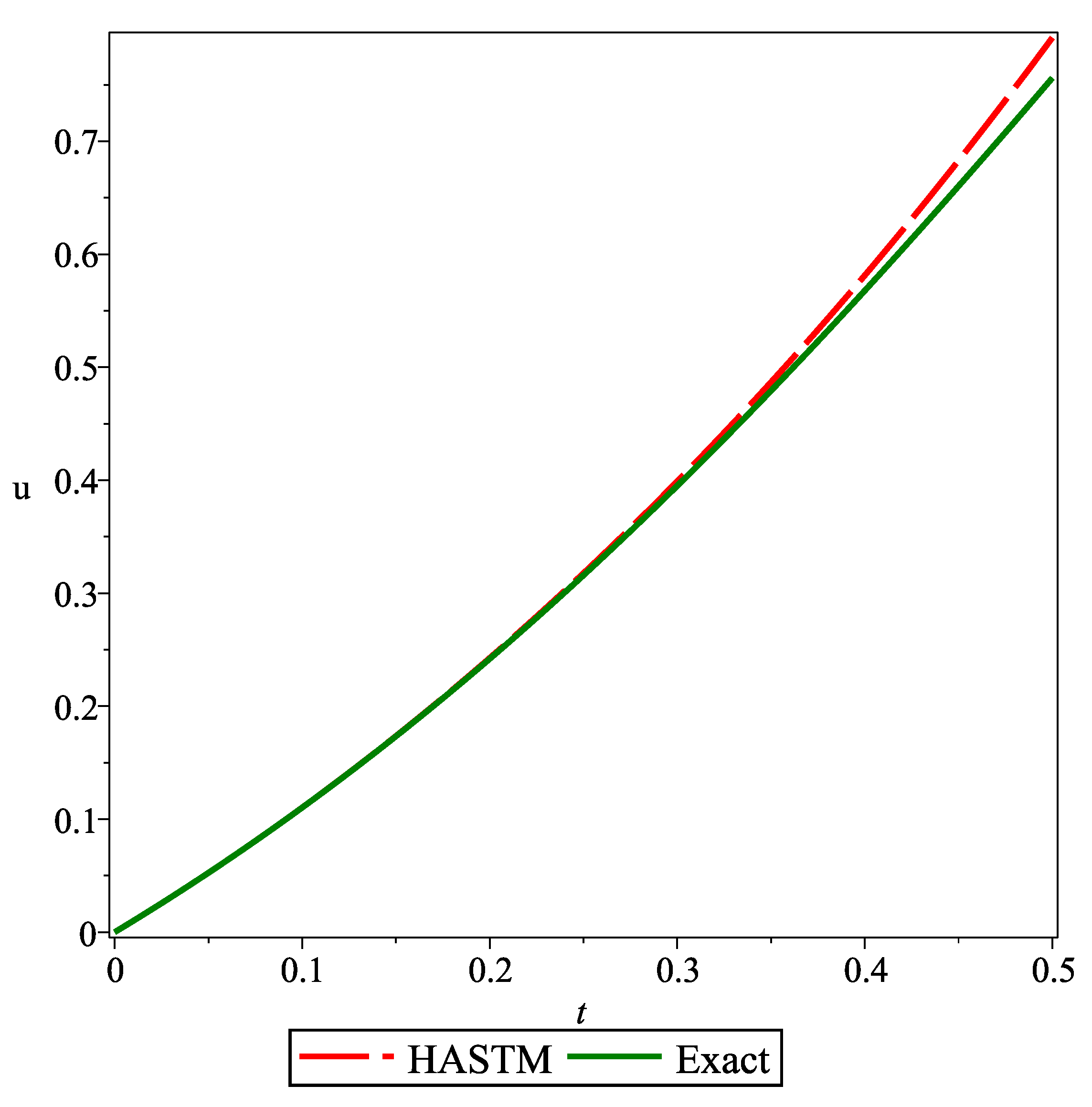
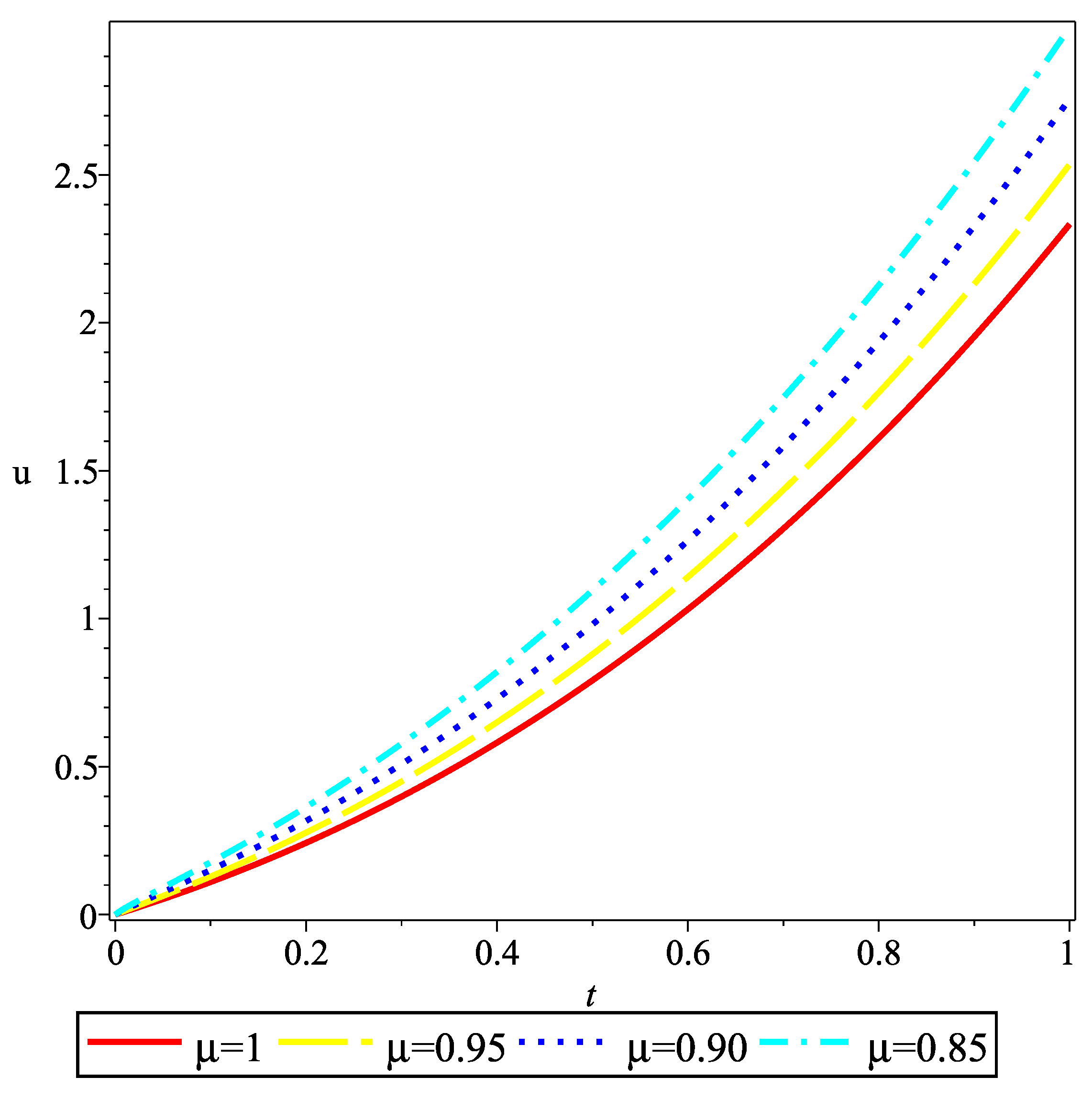
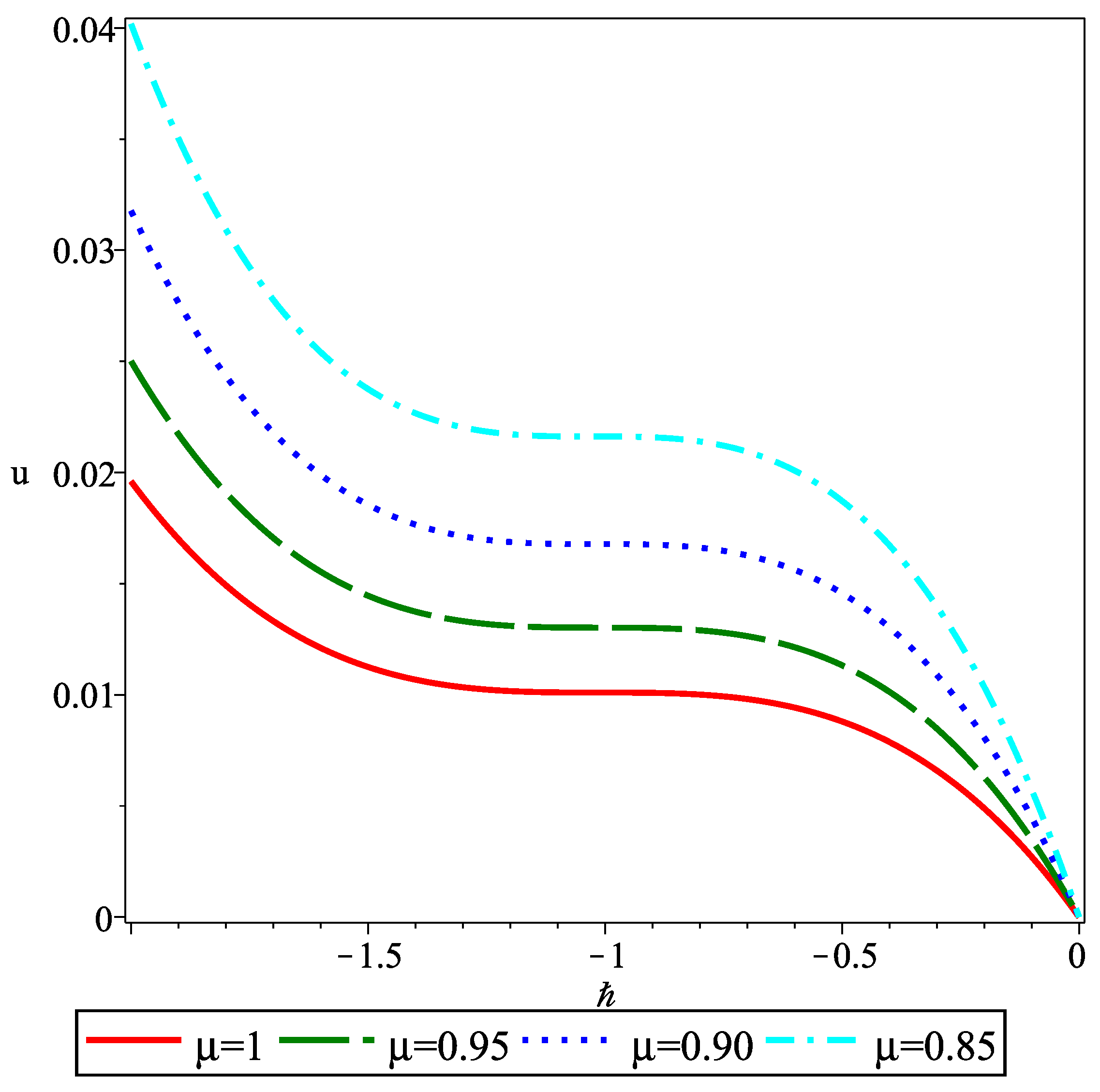
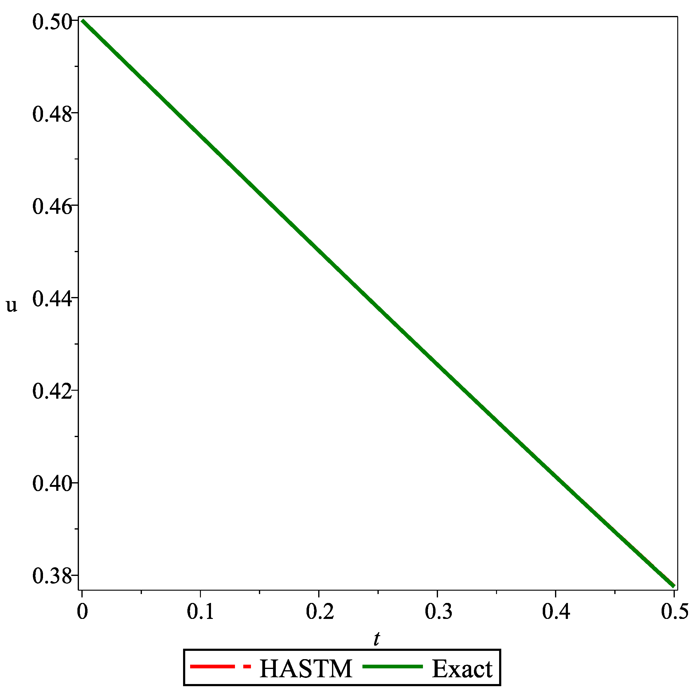
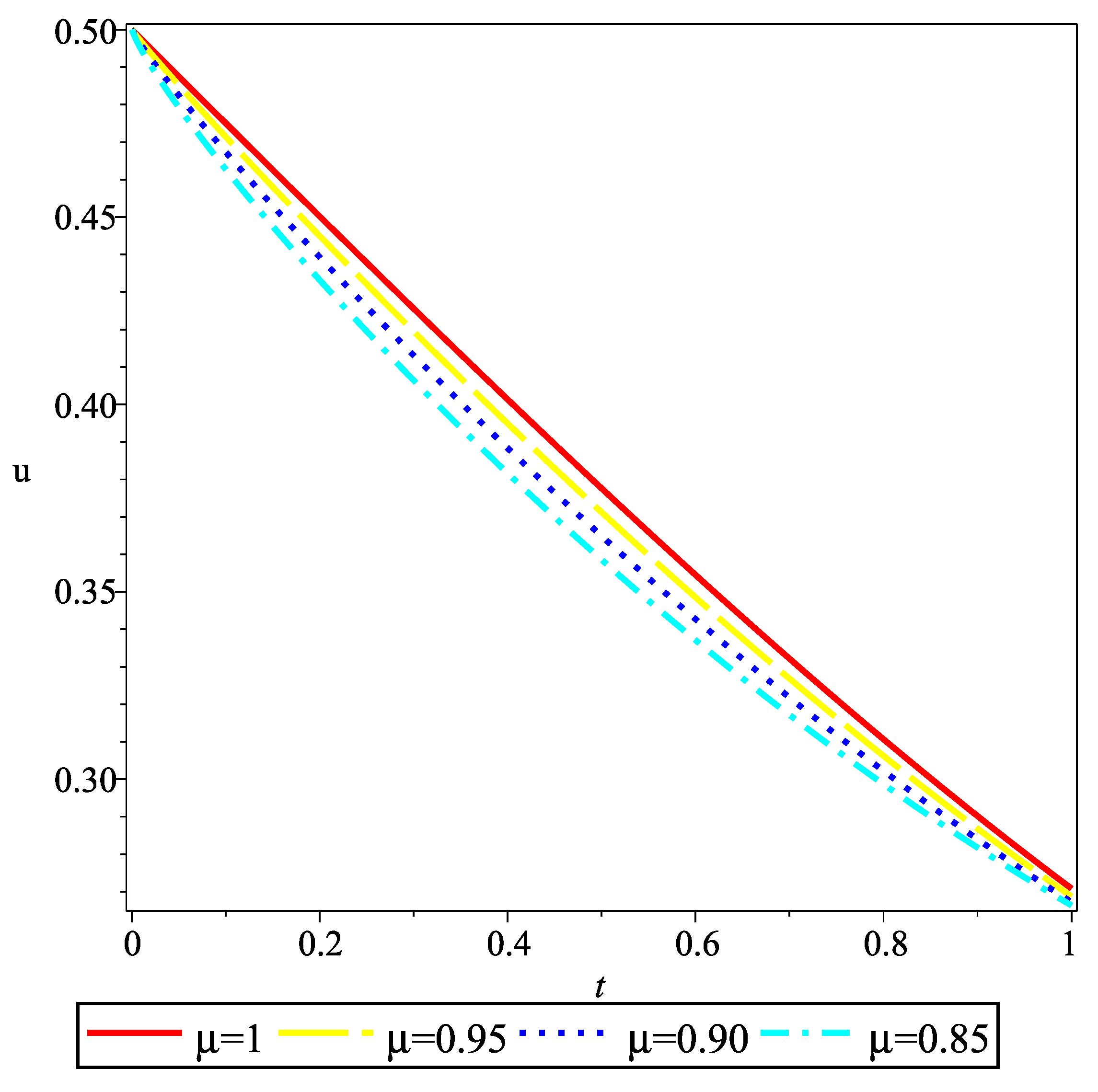
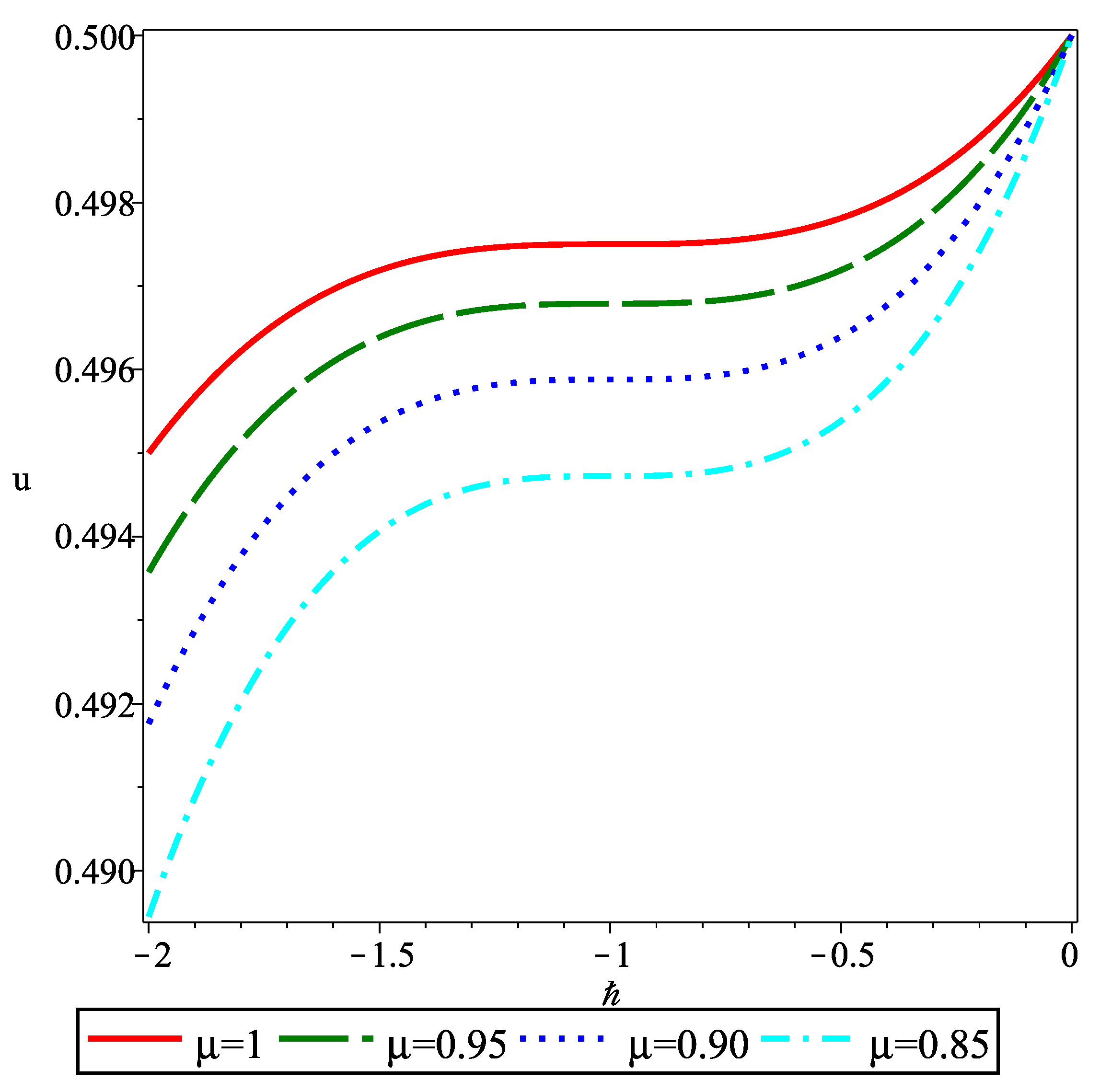
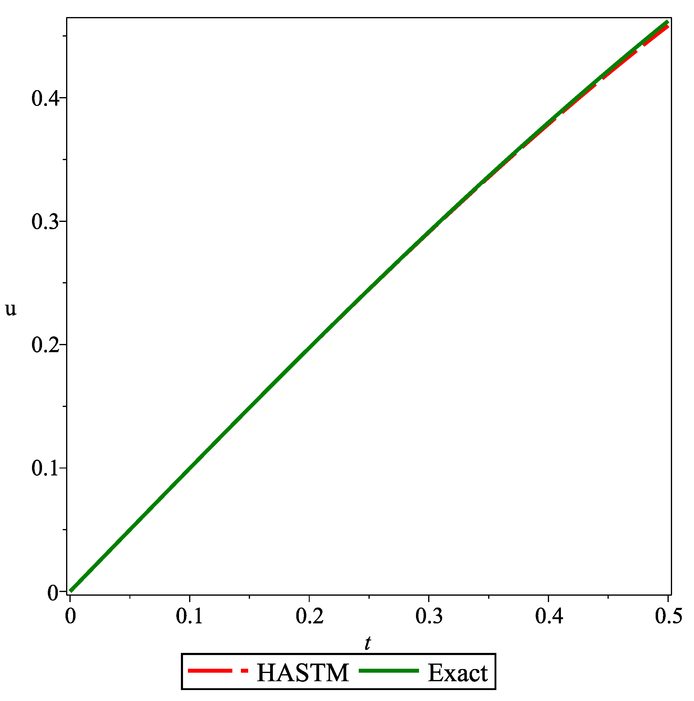
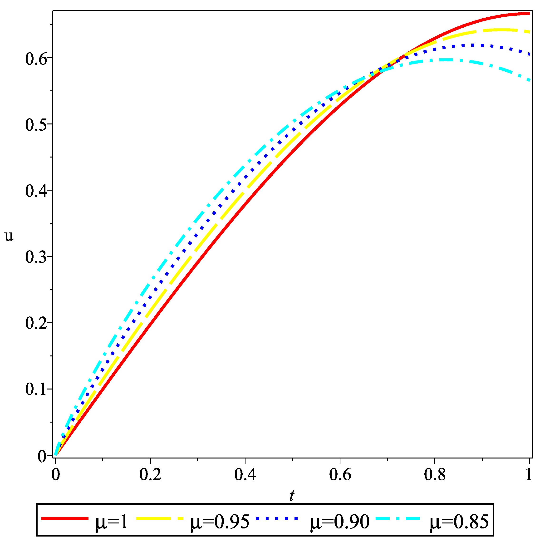
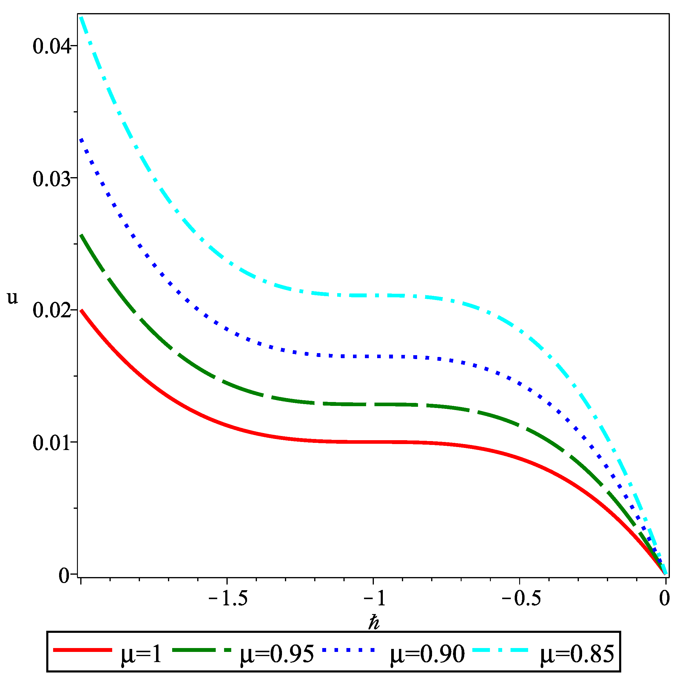
6. Numerical Outcomes

Here, we perform numerical simulations by utilizing the applied method, i.e., the HASTM for the solution to the FRD equation at $\mu =0.95,\mu =0.90$, $\mu =0.85$, and additionally for $\mu =1$. The results of this numerical simulation are provided in the form of

Table 1. Comparative analysis of the numerical results for $u\left(t\right)$ at $\hslash =-1$ and $\mu =1$ for Example 1.

t	Exact Solution	HASTM	Variation in Parameters Method [32]	Homotopy Perturbation Method [32]	Error of HASTM
0.0	0.000000	0.000000	0.000000	0.000000	0
0.2	0.2419767992	0.2426666667	0.2419499764	0.2419648204	6.8986 × 10${}^{-4}$
0.4	0.5678121656	0.5813333333	0.5673979034	0.5681149562	1.3521 × 10${}^{-2}$
0.6	0.9535662155	1.032000000	0.9525886597	0.9582588343	7.8434 × 10${}^{-2}$
0.8	1.346363655	1.610666667	1.345789984	1.365239549	2.6430 × 10${}^{-1}$
1.0	1.689498390	2.333333333	1.688651308	1.723809524	6.4383 × 10${}^{-1}$

,

Table 2. Comparative analysis of the numerical results for $u\left(t\right)$ at $\hslash =-1$ and $\mu =1$ for Example 2.

t	Exact Solution	HASTM Solution	New Homotopy Perturbation Method [8]	Trignometric Transform Method [33]	Error of HASTM
0.0	0.5000000000	0.5000000000	0.5000000000	0.500000	0
0.2	0.4501660027	0.4501666667	0.4501653361	0.450065	6.640 × 10${}^{-7}$
0.4	0.4013123399	0.4013333333	0.412910065	0.401178	2.099 × 10${}^{-5}$
0.6	0.3543436938	0.3545000000	0.3541816941	0.354203	1.563 × 10${}^{-4}$
0.8	0.3100255189	0.3106666667	0.3093428632	0.309897	6.411 × 10${}^{-4}$
1.0	0.2689414214	0.2708333333	0.2668582870	0.268837	1.892 × 10${}^{-3}$

and

Table 3. Comparative analysis of the numerical results for $u\left(t\right)$ at $\hslash =-1$ and $\mu =1$ for Example 3.

t	Exact Solution	HASTM Solution	Fractional Variational Iteration Method [10]	Modified Homotopy Perturbation Method [10]	Trignometric Transform Method [33]	Error of HASTM
0.0	0	0	0	0	0	0
0.2	0.1973753203	0.1973333333	0.197375	0.197375	0.197773	04.1987 × 10${}^{-5}$
0.4	0.3799489622	0.3786666667	0.380005	0.379944	0.380422	1.28229 × 10${}^{-3}$
0.6	0.5370495670	0.5280000000	0.537923	0.536857	0.537449	9.0496 × 10${}^{-3}$
0.8	0.6640367702	0.6293333333	0.669695	0.661706	0.664037	3.4703 × 10${}^{-2}$
1.0	0.7615941560	0.6666666667	0.784126	0.746032	0.761671	9.4927 × 10${}^{-2}$

and Figure 1, Figure 2, Figure 3, Figure 4, Figure 5, Figure 6, Figure 7, Figure 8 and Figure 9. The comparative study of the results obtained by the implemented method, the exact solution, and other methods are shown in Table 1, Table 2 and Table 3. Figure 1 (for Example 1), Figure 4 (for Example 2), and Figure 7 (for Example 3) represent the solution to $u\left(t\right)$ obtained using the HASTM and the exact solution for$\mu =1$. These figures show that the solution obtained by the implemented method was quite close to exact solution. Figure 2 (for Example 1), Figure 5 (for Example 2), and Figure 8 (for Example 3) are plotted to show the variation in the approximate solutions of $u\left(t\right)$ for $\mu =0.85,\mu =0.90,\mu =0.95$, and $\mu =1$. From these figures, we can observe that by slightly changing in the value of $\mu$, the graphs maintain their shapes but shift a bit from their positions. Thus, it is noticeable that the solution profiles significantly depend upon the order of the Caputo–Prabhakar operator. Figure 3 (for Example 1), Figure 6 (for Example 2), and Figure 9 (for Example 3) show the ℏ-curves for various values of $\mu$. In this method, the convergence of the obtained solution was handled by ℏ.

7. Conclusions

In this paper, we successfully implemented the HASTM to obtain the approximate solution to the FRD equations. The outcomes of the discussed examples using the HASTM were compared with other methods and the exact solution. The error analysis shown in the table illustrated the accuracy and potential of the implemented technique. The convergence of the obtained solutions was controlled by utilizing the auxiliary parameter ℏ. Hence, we can conclude that the applied technique is accurate and efficient in solving this type of problems in the field of mathematical modeling. This research work is beneficial to the fields of stochastic control, transmission lines, control theory, river flows, and many more. It opens new avenues in these areas.

References

1. Podlubny, I. Fractional Differential Equations; Academic Press: New York, NY, USA, 1999. [Google Scholar]
2. Miller, K.S.; Ross, B. An Introduction to the Fractional Calculus and Fractional Differential Equations; John Wiley and Sons: New York, NY, USA, 1993. [Google Scholar]
3. Oldham, K.B.; Spanier, J. The Fractional Calculus: Theory and Applications of Differentiation and Integration to Arbitrary Order; Academic Press: New York, NY, USA, 1974. [Google Scholar]
4. Kilbas, A.A.; Srivastava, H.M.; Trujillo, J.J. Theory and Applications of Fractional Differential Equations; Elsevier: Amsterdam, The Netherlands, 2006. [Google Scholar]
5. Singh, J.; Gupta, A.; Baleanu, D. On the analysis of an analytical approach for fractional Caudrey-Dodd-Gibbon equations. AlExample Eng. J. 2022, 61, 5073–5082. [Google Scholar] [CrossRef]
6. Goswami, A.; Rathore, S.; Singh, J.; Kumar, D. Analytical study of fractional nonlinear Schrodinger equation with harmonic oscillator. Discrete Contin. Dyn. Syst.—S 2021, 14, 3589–3610. [Google Scholar] [CrossRef]
7. Dubey, V.P.; Kumar, R.; Kumar, D.; Khan, I.; Singh, J. An efficient computational scheme for nonlinear time fractional systems of partial differential equations arising in physical sciences. Adv. Differ. Equ. 2020, 46. [Google Scholar] [CrossRef]
8. Khan, N.A.; Ara, A.; Jamil, M. An efficient approach for solving the Riccati equation with fractional orders. Comput. Math. Appl. 2011, 61, 2683–2689. [Google Scholar] [CrossRef] [Green Version]
9. Geng, F. A modified variational iteration method for solving Riccati differential equations. Comput. Math. Appl. 2010, 60, 1868–1872. [Google Scholar] [CrossRef] [Green Version]
10. Merdan, M. On the solutions Fractional Riccati Differential Equation with Modified Riemann-Liouville Derivative. Int. J. Differ. Equ. 2012, 2012, 346089. [Google Scholar] [CrossRef]
11. Sakar, M.G.; Akgul, A.; Baleanu, D. On solutions of fractional Riccati differential equations. Adv. Differ. Equ. 2017. [Google Scholar] [CrossRef]
12. Ghomanjani, F.; Khorram, E. Approximate solution for quadratic Riccati differential equation. J. Taibah Univ. Sci. 2017, 12, 246–250. [Google Scholar] [CrossRef]
13. Ezz-Eldien, S.S.; Machado, J.A.T.; Wang, Y.; Aldraiweesh, A.A. An algorithm for the Approximate solution of the fractional Riccati Differential Equation. Int. J. Nonlinear Sci. Numer. Simul. 2019, 20, 661–674. [Google Scholar] [CrossRef]
14. Rasedee, A.F.N.; Sathar, H.A.; Ishak, N.; Hamzah, S.R.; Jamaludin, N.A. Numerical Approximation of Riccati type differential equations. ASM Sci. J. 2020, 13. [Google Scholar] [CrossRef]
15. Ranjbar, A.; Hosseinnia, S.H.; Soltani, H.; Ghasemi, J. A solution of Riccati non-linear differential equation using Enhanced Homotopy Perturbation Method (EHPM). Int. J. Eng. Trans. 2008, 21, 27–38. [Google Scholar]
16. Liu, X.; Kamran; Yao, Y. Numerical approximation of Riccati Fractional differential equation in the sense of Caputo-Type Fractional derivative. J. Math. 2020, 2020, 1274251. [Google Scholar] [CrossRef]
17. Tan, Y.; Abbasbandy, S. Homotopy analysis method for quadratic Riccati differential equation. Commun. Nonlinear Sci. Numer. Simul. 2008, 13, 539–546. [Google Scholar] [CrossRef]
18. Singh, J.; Kumar, D.; Baleanu, D.; Rathore, S. An efficient numerical algorithm for the fractional Drinfeld-Sokolov-Wilson equation. Appl. Math. Comput. 2018, 335, 12–24. [Google Scholar] [CrossRef]
19. Prabhakar, T.R. A singular integral equation with a generalized Mittag-Leffler function in the kernel. Yokohama Math. J. 1971, 19, 7–15. [Google Scholar]
20. D’Ovidio, M.; Polito, F. Fractional diffusion-telegraph equations and their associated stochastic solutions. Theory Probab. Appl. 2018, 62, 552–574. [Google Scholar] [CrossRef]
21. Giusti, A.; Colombaro, I.; Garra, R.; Garrappa, R.; Polito, F.; Popolizio, M.; Mainardi, F. A practical guide to prabhakar fractional calculus. Fract. Calc. Appl. Anal. 2020, 23, 9–54. [Google Scholar] [CrossRef] [Green Version]
22. Derakhshan, M.H.; Aminataei, A. Comparison of homotopy perturbation transform method and fractional Adams-Bashforth method for the Caputo-Prabhakar nonlienar fractional differential equations. Iranian J. Numer. Anal. Optim. 2020, 10, 63–85. [Google Scholar]
23. Kilbas, A.A.; Saigo, M.; Saxena, R.K. Generalized Mittag-Leffler function and generalized fractional calculus operators. Integral Transform. Spec. Funct. 2004, 15, 31–49. [Google Scholar] [CrossRef]
24. Garra, R.; Gorenflo, R.; Polito, F.; Tomovski, Z. Hilfer-Prabhakar derivatives and some applications. Appl. Math. Comput. 2014, 242, 576–589. [Google Scholar] [CrossRef] [Green Version]
25. Giusti, A.; Colombaro, I. Prabhakar like fractional viscoelasticity. Comm. Nonlin. Sci. Num. Sim. 2018, 56, 138–143. [Google Scholar] [CrossRef] [Green Version]
26. Watugala, G.K. Sumudu Transform-a new integral transform to solve differential equations and control engineering problems. Int. J. Math. Educ. Sci. Tech. 1993, 24, 35–43. [Google Scholar] [CrossRef]
27. Chaurasia, V.B.L.; Singh, J. Application of Sumudu transform in Schrodinger equation occurring in quantum mechanics. Appl. Math. Sci. 2010, 4, 2843–2850. [Google Scholar]
28. Belgacem, F.B.M.; Karaballi, A.A.; Kalla, S.L. Analytical investigations of the Sumudu transform and applications to integral production equations. Math. Probl. Eng. 2003, 3, 103–118. [Google Scholar] [CrossRef] [Green Version]
29. Panchal, S.K.; Khandagale, A.D.; Dole, P.V. Sumudu transform of Hilfer-Prabhakar fractional derivatives with applications. Proceeding Natl. Conf. Recent Trends Math. 2017, 1, 60–66. [Google Scholar]
30. Odibat, Z.; Bataineh, S.A. An adaptation of homotopy analysis method for reliable treatment of strongly nonlinear problems: Construction of homotopy polynomials. Math. Methods Appl. Sci. 2015, 38, 991–1000. [Google Scholar] [CrossRef]
31. Argyros, I.K. Convergence and Applications of Newton-type Iterations; Springer: New York, NY, USA, 2008. [Google Scholar]
32. Magrenan, A.A. A new tool to study real dynamics: The convergence plane. Appl. Math. Comput. 2014, 248, 215–224. [Google Scholar] [CrossRef] [Green Version]
33. Haq, E.U.; Ali, M.; Khan, A.S. On the solution of fractional Riccati differential equations with variation of parameters method. Eng. Aappl. Sci. Lett. 2020, 3, 1–9. [Google Scholar]
34. Agheli, B. Approximate solution for solving fractional Riccati differential equations via trignometric basic functions. Trans. A Razmadze Math. Inst. 2018, 172, 299–308. [Google Scholar] [CrossRef]
Figure 1. Plot of u ( t ) with respect to t for μ = 1 .
Mathematics 11 00644 g001
Figure 2. Response of u ( t ) with respect to t for distinct values of μ .
Mathematics 11 00644 g002
Figure 3. -curve of u ( t ) at t = 0.01 for various values of μ .
Mathematics 11 00644 g003
Figure 4. Plot of u ( t ) with respect to t for μ = 1 .
Mathematics 11 00644 g004
Figure 5. Response of u ( t ) with respect to t for distinct values of μ .
Mathematics 11 00644 g005
Figure 6. -curve of u ( t ) at t = 0.01 for various values of μ .
Mathematics 11 00644 g006
Figure 7. Plot of u ( t ) with respect to t for μ = 1 .
Mathematics 11 00644 g007
Figure 8. Response of u ( t ) with respect to t for distinct values of μ .
Mathematics 11 00644 g008
Figure 9. -curve of u ( t ) at t = 0.01 for various values of μ .
Mathematics 11 00644 g009