The Relative Distance Prediction of Transmembrane Protein Surface Residue Based on Improved Residual Networks

Abstract

(1) Background: Transmembrane proteins (TMPs) act as gateways connecting the intra- and extra-biomembrane environments, exchanging material and signals crossing the biofilm. Relevant evidence shows that corresponding interactions mostly happen on the TMPs’ surface. Therefore, knowledge of the relative distance among surface residues is critically helpful in discovering the potential local structural characters and setting the foundation for the protein’s interaction with other molecules. However, the prediction of fine-grained distances among residues with sequences remains challenging; (2) Methods: In this study, we proposed a deep-learning method called TMP-SurResD, which capitalized on the combination of the Residual Block (RB) and Squeeze-and-Excitation (SE) for simultaneously predicting the relative distance of functional surface residues based on sequences’ information; (3) Results: The comprehensive evaluation demonstrated that TMP-SurResD could successfully capture the relative distance between residues, with a Pearson Correlation Coefficient (PCC) of 0.7105 and 0.6999 on the validation and independent sets, respectively. In addition, TMP-SurResD outperformed other methods when applied to TMPs surface residue contact prediction, and the maximum Matthews Correlation Coefficient (MCC) reached 0.602 by setting a threshold to the predicted distance of 10; (4) Conclusions: TMP-SurResD can serve as a useful tool in supporting a sequence-based local structural feature construction and exploring the function and biological mechanisms of structure determination in TMPs, which can thus significantly facilitate the research direction of molecular drug action, target design, and disease treatment.

1. Introduction

Transmembrane proteins (TMPs) are the intermediary between the two sides of biological membranes [1]. Cells use TMPs to transduce signals into cells, transport ions and molecules, bind the cell to a surface or substrate, and catalyze reactions [2]. They are also widely involved in various human diseases and are undoubtedly the primary drug target resource [3,4]. The evidence pointing toward TMPs’ surface is highly related to such different physiologic functions because they form the structural preferences of their binding pocket for drugs or other biological molecules [5], and corresponding interactions mostly happen on TMPs’ surface [6] which are mediated by highly conserved residues in adjacent [7,8].

The interaction involves residues on the surface that are close to each other in the spatial conformation but may separate on the protein sequence [9]. Accurate knowledge of the relative distance between surface residues of TMPs is a meaningful study for biological problems such as functional annotation, structural modeling, and drug discovery [10]. However, the number of TMPs with determinate experimental structures in the RCSB PDB [11] is less than 2% [12] and the accuracy of predicted structures by AlphaFold [13] has yet to be verified. Therefore, it is still more difficult to be engaged in relevant TMP research directly from the perspective of structures at present. Fortunately, the sequence data of TMPs have emerged in large quantities with the development of high-throughput sequencing technology. It is necessary to develop a predictor based on sequences for calculating the relative distance of residues to meet the needs of local structure research in this context. Limited by prior knowledge and calculation methods, many previous researchers were interested in the studies of residue contact [14,15], while little attention was paid to residue distances [16]. Nevertheless, the contact-based prediction has gradually reached the performance ceiling. It cannot wholly reflect the relative position information of residues in a stable spatial conformation, such as chiral molecules and dihedral angles. Recently, some new methods have been proposed to predict the inter-residue distance [17,18,19] as a crucial intermediate step to achieving the overall goal of effectively optimizing protein folding from the sequence [20,21,22], but unanimously by simplifying the residue distance into residue contact. However, what we are interested in is often different from the distances between all residues on the whole sequence and the relative positions of residues in local regions in a specific task because enough guidance can be provided for local structural feature extraction or other downstream work.

In this study, a regression-based distance prediction method is proposed, named TMP-SurResD, which adopts the improved residual network to capture the delicate geometric relationship between residue pairs and thus could predict the continuous and relative distance of functional surface residues rapidly and satisfactorily. Some feature profiles of TMPs based on their primary sequences firstly were constructed, including sequence coding, evolutionary conservation, coevolution information derived by sequence alignment, and relative solvent accessibility. Next, we designed a multi-channel feature extractor to learn the latent information from these physicochemical and biochemical profiles based on the combination of the Residual Block (RB) [23] and Squeeze-and-Excitation (SE) [24]. The RB learned features by integrating spatial and channel information, and the SE focused on the relationship between channels, aiming to discover the importance of different channel features automatically. TMP-SurResD exploited this integration block to extract local and global information fully.

Furthermore, the distance matrix is normalized to reduce the training error caused by the wide range of maximum residual distance distribution. The sequence-based features extracted were input into the model through different combinations to explore the contribution of additional features and combinations. Finally, we demonstrated that TMP-SurResD significantly outperformed other state-of-the-art methods through a comprehensive evaluation of an independent test data set and could accurately identify residue distances based on sequence-based input information. The rich and multi-level supervision information gave TMP-SurResD a highly fitting ability. Moreover, we hope this study will set the groundwork for this important topic and suggest future directions and applications. TMP-SurResD is freely accessible at https://github.com/NENUBioCompute/TMP-ResDistancePre (accessed on 3 January 2023).

2. Materials and Methods

The TMP-SurResD’s pipeline is shown in Figure 1, where Figure 1a shows the collection and preprocessing of the benchmark datasets, Figure 1b illustrates the details about extracting the four features, Figure 1c describes how features in different dimensions are combined, and the details about deep learning model are shown in Figure 1d.

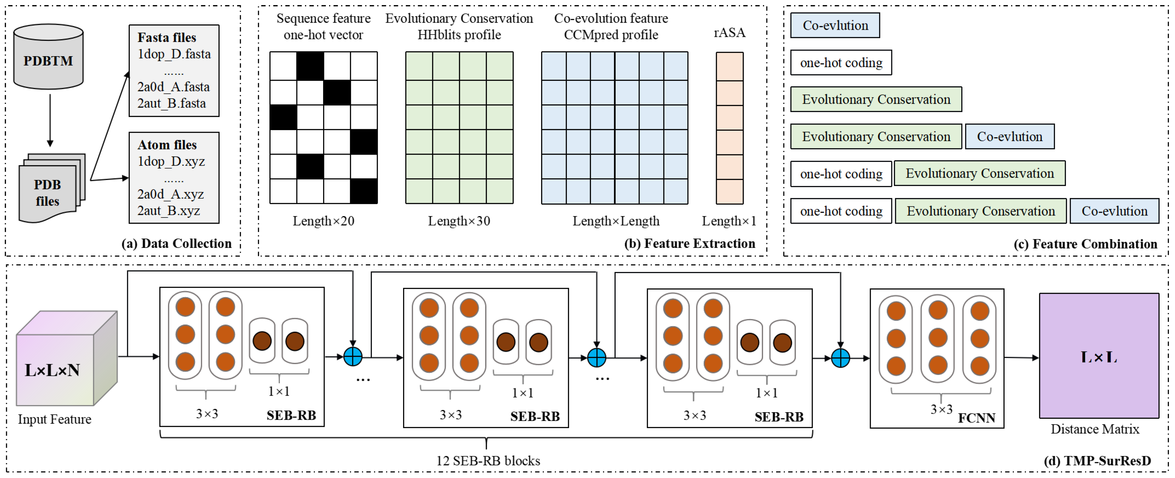
2.1. Benchmark Dataset

6509 TMP complexes were downloaded from PDBTM (version: 2021-10-01) [25]. Biopython was then used to parse 33,458 redundant protein sequences and 3D coordinates of C$\alpha$ atoms for each residue from PDB files. The protein chains containing multiple identifier alignments that cannot be identified were removed, and we retained the sequences composed of 20 standard amino acids in a particular order. We also removed the chains whose length was less than 30 residues or the long sequence over 1000. Since short sequences may not fold into a representative structure, long sequences bring training difficulties to the model. After data pre-processing, CD-HIT [26] was utilized to eliminate the same structures with a 30% sequence identity cut-off to maintain low homology among sequences, resulting in 887 $\alpha$-TMP chains left. We denoted the remaining chains as SurTotal.

The whole sequence features are used as the model’s input to retain the information distributed on the original sequences as entirely as possible and make them have biological significance. Furthermore, to evaluate the effectiveness of TMP-SurResD, the protein sequences were randomly divided into a training set (SurTrain) of 532 TMP sequences, a validation set (SurValid) of 177, and an independent test set (SurTest) of 178 in a 6:2:2 ratio and their sequence distribution length is consistent. SurTrain, SurValid, and SurTest are used to train the model weights, determine the learning rate and test the final performance of the network, respectively [27].

2.2. Protein Sequence Descriptors

Previous residue contact prediction relies mainly on information derived from sequences [18]. We can also obtain a great many derivative features from sequences for reference, such as physicochemical properties [28], amino acid composition [29], and secondary structure [30]. However, not all features positively promote the prediction of residues distances, and some features have the opposite effect. In this study, we finally extracted four features to characterize the structure of TMPs from different perspectives: sequence coding, evolutionary conservation, coevolution information, and relative solvent accessibility.

2.2.1. Sequence Encoding

The one-hot encoding (OH) scheme is popular since deep learning models require grid-like input with numbers [31]. Simultaneously, protein sequences encoded with OH have been successfully applied to the related task of protein structure prediction [32]. A sequence is transformed into a sparse matrix of size $L\times N$ [33], where L represents the sequence length, and N denotes 20 amino acid types.

2.2.2. Evolutionary Conservation

Evolutionary conservation (EC) employed in many bioinformatics problems is identified by aligning the amino acid sequences of proteins with the same function from different taxa (orthologs), which ca n help to determine the folding patterns of spatial structures and infer potential functional surfaces of protein molecules. Highly conserved regions in a protein during evolution are always functional regions [34]. Here we employed HHblits [35] to generate the suffix ‘.hhm’ files by searching against the uniprot20_2016_02 database with three iterations and a 0.01 E-value cut-off. Eventually, for a given TMP sequence, the EC feature extracted from the ‘.hhm’ file is a 30-dimension matrix, with each column representing a profile and each row representing a residue. It must be normalized using the Formula (1) to distribute it evenly in [0, 1] to avoid the deviation of the extensive distribution of each value ranging from 0 to 9999. An HHM represents this feature.

$$f\left(x\right)=\frac{1}{1+e^{-\frac{x}{200}}}$$

(1)

2.2.3. Co-Evolutionary Information

The co-evolutionary pressure to maintain a stable protein structure gives rise to correlated mutations between contacting residue pairs. The coevolution among residues can be observed using multiple sequence alignments (MSAs generated by DeepMSA [36]) of the protein family and can be used to predict residue-residue distance. Currently, the state-of-the-art methods for residue distance prediction all utilize co-evolutionary patterns directly or indirectly. The indirect strategy is to construct MSA for the targeisrotein sequence [37] and then extract the potential patterns of residue pairs in the MSA. The application, CCMPred [38], was chosen to disentangle direct couplings for all residue pairs of each TMP from mere correlations between MSA columns. Among them, CCMPred applies the Potts statistical models [39] that can distinguish direct couplings between pairs of columns in multiple sequence alignments from merely correlated pairs to obtain the covariance matrix, thereby obtaining the $L\times L$ co-evolutionary coupling information, and this feature will be referred to as CCM.

2.2.4. Relative Solution Accessibility

Solvent-exposed residues can interact directly with other biomolecules. Specifically, the hydrophobic residues buried in the structure and the hydrophilic residues exposed in the solvent reach an equilibrium to form a hydrophobic effect, and the hydrophobic force makes the polypeptide chain overcome the entropy factor in the solvent and enter a folded state [40]. The relative solvent accessible surface area (rASA) is generated by dividing the accessible location of each residue molecule by the maximum accessible surface area of the protein. TMP-SSurface2 [5] is efficient in predicting the surface of TMPs, which took one-hot coding and position-specific scoring matrix (PSSM) [41] as input. Based on the predicted value, residues were divided into two categories. A value less than 0.2 indicates that the residue is exposed to the solvent. Otherwise, it is buried internally. Consequently, a matrix of size $L\times 1$ is obtained.

2.3. The Representation of Residue Distance

From the perspective of data input and output format, the problem of TMP residue distance prediction is analogized to the monocular image depth prediction in three-dimensional (3D) perception [42,43]. The purpose of these is considered as the regression problem of disparity maps. Monocular image depth prediction is to obtain the geometric features of 3D scenes from two-dimensional (2D) images [44]. The input volume has dimensions $H\times W\times D$ (height, width, and depth, respectively), and the output is the depth information of size $H\times W$ [45]. Similarly, the residue distance prediction input is $L\times L\times N$, which outputs a distance map of $L\times L$. Image depth prediction usually involves three channels (red, green, and blue), while the difference is that there are more features in the latter, such as 56 or 441 channels [42] or even more.

2.3.1. Feature Combination

Dimension transformation is usually required when the feature dimensions are inconsistent in the feature processing stage. Taking the combination of one-hot coding, HHM, and CCM as an example, the specific methods of combining them to adapt to the model input are shown in Formulas (2) to (4). Firstly, the two features are horizontally stacked to convert an OHH. Further, a single residue feature is obtained through the outer concatenate operation and then reshaped into a 3D residue pairs feature OHHP. Finally, it is stacked horizontally with the remaining CCM in depth.

$$OHH=hstack(OH,HHM)$$

(2)

$$OHHP[i,j,:]=reshape\left(concat\right(OHH[i,:],OHH[:,j]\left)\right)$$

(3)

$$OCC[i,j,:]=concat\left(OHP\right[i,j,:],CCM[i,j,:\left]\right)$$

(4)

2.3.2. Label Matrix Generation

To label the training samples, we extracted the coordinates of C$\alpha$ on the residue backbone from the PDB files and calculated the spatial distance between C$\alpha$-C$\alpha$ using Equation (5).

$$|A_i{B}_j|=\sqrt{{(x_i-x_j)}^2+{(y_i-y_j)}^2+{(z_i-z_j)}^2}$$

(5)

Since we are interested in the surface residues on TMP, the feature of rASA was used to filtrate out the surface residues. A particular way is that atom files with the coordinates of C$\alpha$ were associated with rASA files via PDB identifications. Each C$\alpha$ atom in the PDB file was traversed, and if the rASA value of the residue was less than 0.2, it failed to participate in the distance calculation. Because the statistical analysis found that the maximum value of the distance value distribution range was 30 to 200, we took advantage of Equation (6) to normalize each value to be between 0 and 1, where Min and Max were assigned the values 0 and 200, respectively.

$$x^{\prime }=\frac{x-Min}{Max-Min}=\frac{x}{200}$$

(6)

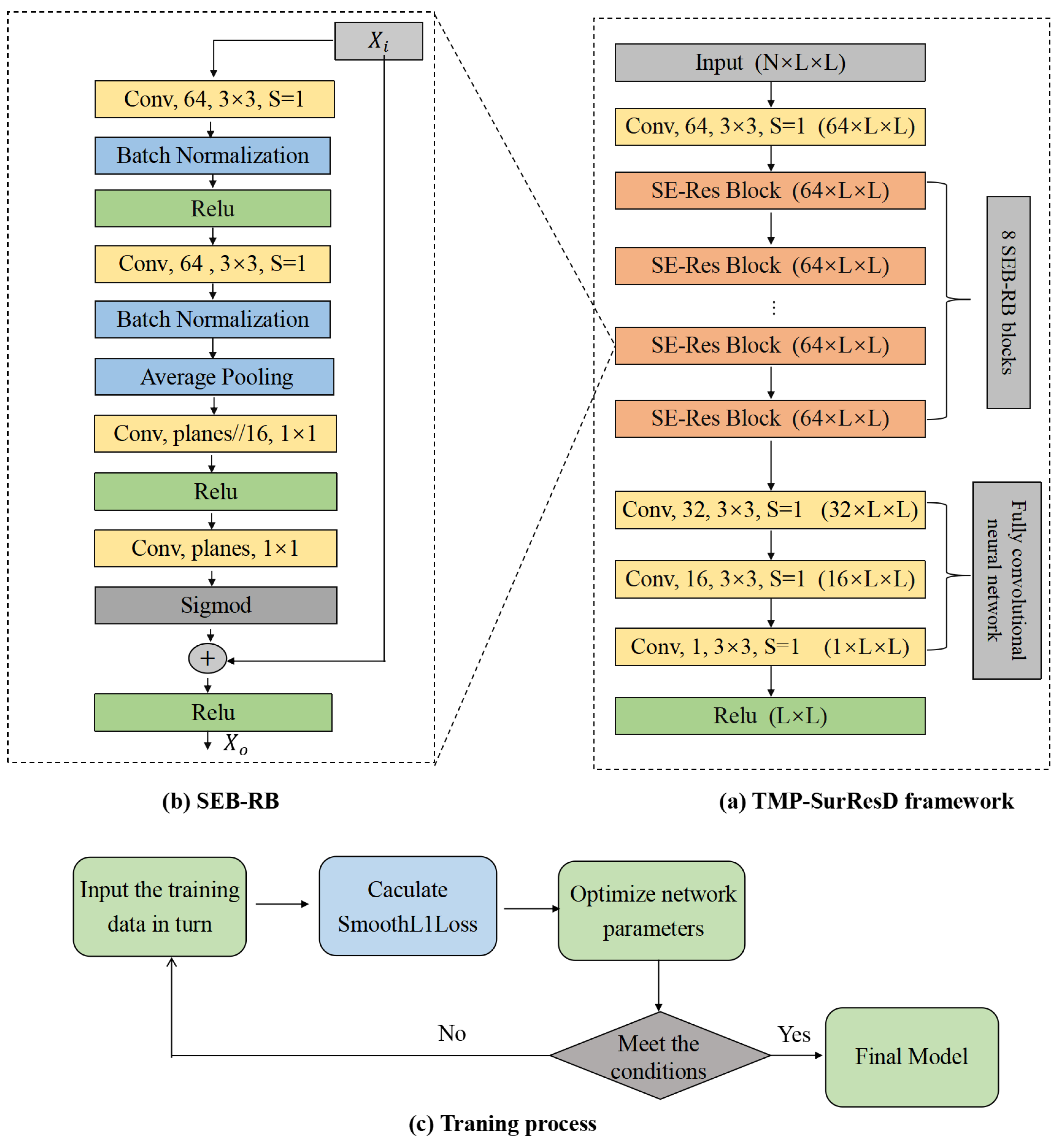
2.4. Deep Learning Model Details

2.4.1. Model Design

As shown in Figure 2a, the network adopts the serial integration technique, which consists of 12 SEB-RB blocks of the same structure and a full convolutional neural network (FCNN) [46] stacked sequentially. The input = $L\times L\times N$ first goes through a convolutional layer with a convolution kernel size = $3\times 3$ and stride = 1, where N varies according to the features. For example, when OH is used, N is 40; when OH and CCM are composed, N is $41\times (40+1)$; when all features (OH+HHM+CCM) are combined, N is $101\times (40+60+1)$. The filters are set to 64, which can reduce the dimension of the number of channels. The latent representation of the data then goes through 12 SEB-RB blocks and enters three convolutional neural layers for decoding operations. The last three filters are set to 64, 32, 16, and 1, respectively. Finally, the relative distance matrix of $L\times L$ is output after being activated by ReLU [47].

The SEB-RB block, as mentioned above, is composed of the squeeze-and-excitation block (SEB) [24] and the residual block (RB) [48], where the SEB is embedded in the learning branch of the RB. Incredibly, two original fully connected layers in the SEB were replaced with two 2D convolution layers, and the average pooling layer and sigmoid layer were retained in the latter part of SEB-RB. Pooling and dense layers are not used in our framework. Therefore, TMP-SurResD can allow sequences of arbitrary length as input. Figure 2b shows the details of the SEB-RB block, and mathematics is defined as the Formula (7). SEB-RB block has such an advantage that it can not only extract features by fusing spatial and channel information but also improve model expression ability from a channel perspective, realizing the extraction of potential interaction patterns between residue pairs in input data from all aspects.

$$X_o=F(X_i,\left\{W_i\right\})+X_i$$

(7)

where $X_i$ and $X_o$ denote the inputs and outputs of this block; $W_i$ and F represent the weights and residual maps to be learned, respectively.

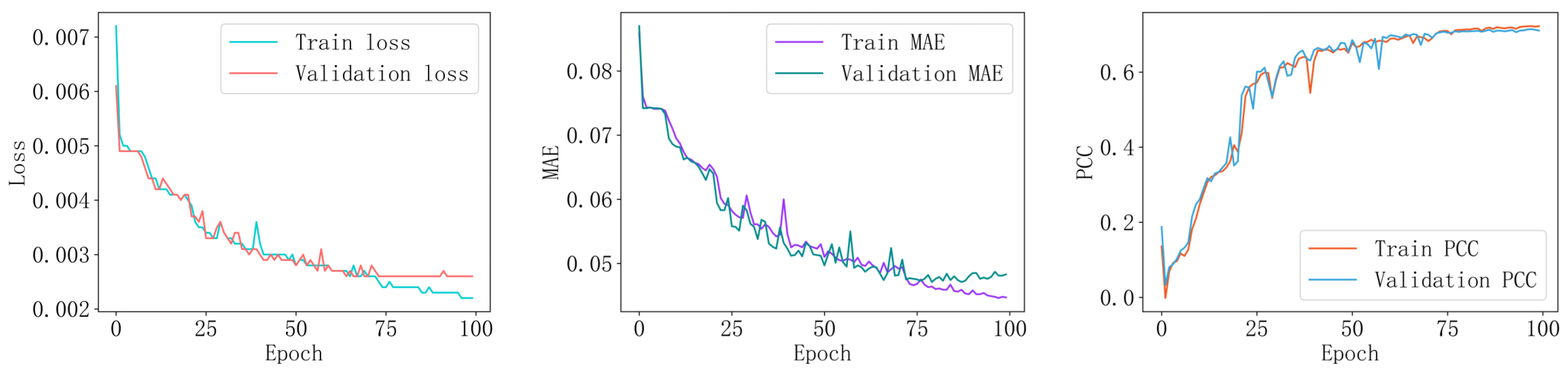
2.4.2. Model Training

TMP-SurResD was developed using the high-performance deep-learning framework Pytorch [49] based on Python 3.6. It statistically took about 20 h to train 100 epochs without using any data and model parallel. During model training, as shown in Figure 2c, batch size and the learning rate were set to 1 and 0.002 in our experiment, respectively. SmoothL1Loss is used to calculate the loss value. Compared with L1-Loss and L2-Loss alone, it has the advantages of making the model more robust to outliers and controlling the magnitude of gradients. Using Adamax [50] to update the network weights is based on the infinite norm and has all the advantages of Adam [50]. TMP-SurResD stopped training when the loss value on SurValid had not changed for 20 consecutive epochs and selected the evaluation indicator corresponding to the output of the last epoch. Finally, Pearson product-moment Correlation Coefficient (PCC) [51] was used to evaluate the overall predictive performance of our model.

2.5. Performance Metrics

The prediction of the distance among residues is a typical regression problem. In regression problems, the effect of regression is usually viewed from two different perspectives: (1) whether the correct value is predicted; (2) whether enough information is fitted. From these two perspectives, PCC, mean absolute error (MAE), and mean square error (MSE) were used to measure the performance of TMP-SurResD. The formulas are defined in (8) to (10).

$$MAE=\frac{1}{n}{\sum }_{i=1}^n\left|y_i-x_i\right|$$

(8)

$$MSE=\frac{1}{n}{\sum }_{i=1}^n{(y_i-x_i)}^2$$

(9)

$$PCC=\frac{{\sum }_{i=1}^n(x_i-\overline{x})(y_i-\overline{y})}{\sqrt{\left[{\sum }_{i=1}^n{(x_i-\overline{x})}^2\right]\left[{\sum }_{i=1}^n{(y_i-\overline{y})}^2\right]}}$$

(10)

Assume that the real distance of all residue pairs on a TMP sequence of length L is $X=[x_1,x_2,\dots x_{n-1},x_n]$, and the predicted distance is $Y=[y_1,y_2,\dots ,y_{n-1},y_n]$. Where N is equal to $L^2$, $x_i$ and $y_i$ denote the observed and predicted distances between any pair of residues severally; $\overline{x}$ and $\overline{y}$ represent the average values of X and Y, respectively.

3. Results

3.1. Characteristic Validity Analysis

It is well known that the upper limit of deep learning performance is determined by the model structure’s complexity and the input characteristics’ validity [5]. The aggregation of residues will change the average action field and become a driving force for protein folding and structural stability [52]. Many residues interact with each other, and the two-body interactions between residues do not exist independently but are often dependent on the surrounding environment [53]. However, inputting the two target residues’ eigenvectors may lack direct biological significance in the prediction model. In addition, in the absence of enough TMP training samples to fit the weight parameters, it is not optimal to take all features as the input simultaneously. Therefore, it is significant to explore the validity of features combination. As can be seen from

Table 1. Prediction performance based on individual input features and their various combinations ¹.

Features	TraMAE	TraMSE	TraPCC	ValMAE	ValMSE	ValPCC
OH	0.0358	0.1254	0.7920	0.0759	0.0102	0.2016
HHM	0.0637	0.0079	0.3378	0.0645	0.0081	0.3321
CCM	0.0387	0.0036	0.7706	0.0447	0.0049	0.7315
OH+HHM	0.0602	0.0067	0.3483	0.0698	0.0089	0.3256
OH+CCM	0.0306	0.0018	0.8586	0.0566	0.0067	0.5888
HHM+CCM	0.0472	0.0048	0.6983	0.0506	0.0062	0.6825
OH+HHM+CCM	0.0422	0.0038	0.7253	0.0504	0.0059	0.6864

¹ Here, we tested the performance of the single feature and multiple feature combinations. To study the contribution of different features, our network structure was initially set to eight SEB-RB blocks. The abbreviation OH in the table represents the one-hot encoding of a single residue; HHM and CCM stand for evolutionarily conservative and co-evolution, respectively. TraMAE, TraMSE, TraPCC, ValMAE, ValMSE, and ValPCC respectively represent MAE, MSE, and PCC on SurTrain and SurValid.

, each feature contains valuable information about the distances of surface residues. When OH and HHM are combined with CCM respectively, the model can achieve excellent predictive performance on SurValid. It is due to CCM revealing a relationship pattern about two residues close to each other in spatial structure always tend to co-evolve, which possesses highly evolutionary information. It demonstrated that residues are spatially close together, providing the most potent interaction.

3.2. Network Structure Analysis

When designing deep learning models, the layers and filter numbers of the network will usually be taken into account simultaneously to achieve a balance of network because both strategies increase the number of parameters that can be learned, expanding the network’s fitting power. By referring to other research and considering the time-computing resources, the only parameter in our work to be adjusted is the number of convolutional layers. Using this approach can generally roughly search for the local optimal model.

Table 2. Effect of the number of SEB-RB blocks ¹.

SEB-RB Blocks	TraMAE	TraMSE	TraPCC	ValMAE	ValMSE	ValPCC
5	0.0925	0.0163	0.1757	0.0921	0.0137	0.2166
6	0.0470	0.0048	0.6965	0.0492	0.0055	0.6877
7	0.0482	0.0051	0.6932	0.0490	0.0054	0.6837
8	0.0472	0.0048	0.6983	0.0506	0.0062	0.6825
9	0.0471	0.0047	0.6972	0.0493	0.0058	0.6980
10	0.0483	0.0051	0.6932	0.0484	0.0054	0.6884
11	0.0463	0.0047	0.7091	0.0474	0.0052	0.7013
12	0.0447	0.0045	0.7222	0.0483	0.0052	0.7105
13	0.0458	0.0046	0.7173	0.0480	0.0055	0.6973
14	0.0433	0.0041	0.7243	0.0481	0.0055	0.6991
15	0.0470	0.0048	0.7030	0.0481	0.0054	0.6942
16	0.0449	0.0044	0.7225	0.0489	0.0056	0.6997
17	0.0425	0.0040	0.7335	0.0464	0.0052	0.7104

¹ See Figure 2b for details about SEB-RB blocks. The initial value of the network structure is 5. Keeping the number of FCNN layers the same, we stacked the SEB-RB block sequentially.

shows how many SEB-RB blocks affect the performance of TMP-SurResD. Since the residue distance prediction problem has more complex input characteristics, the contexts fed into the proposed deep learning model rely on the depth of the network. Furthermore, the prediction accuracy would be directly influenced by its value. The training time increases as the network layer becomes profound, but the model’s prediction performance decreases gradually. A reversal occurs when blocks are 17. As can be seen, the PCC on SurValid is the largest when SEB-RB blocks are set to 12. We also observe that when SEB-RB blocks are 17, the performance is the same as 12, but the former takes statistically 10 hours longer than the latter. Therefore, from careful consideration of training parameters, time, and performance, TMP-SurResD comprises 12 SEB-RB blocks and a fully convolutional neural network containing three convolutional layers.

Similarly, the final FCNN plays the role of channel dimensionality reduction, so it is also an important parameter. We successively tried different values to find the best convolutional layers of FCNN. As seen in

Table 3. Effect of FCNN layers on model performance when the SEB-RB blocks are 12.

Layers	TraMAE	TraMSE	TraPCC	ValMAE	ValMSE	ValPCC
1	0.0438	0.0042	0.7170	0.0478	0.0054	0.6911
2	0.0474	0.0048	0.6952	0.0509	0.0062	0.6726
3	0.0447	0.0045	0.7222	0.0483	0.0052	0.7105
4	0.0456	0.0046	0.7161	0.0470	0.0054	0.7061

, when the number of layers changes, the model’s prediction accuracy will immediately be affected, and three layers (i.e., The kernel sizes are all three and the output channels are 32, 16, and 1, respectively) are best. However, the model’s prediction accuracy may not grow as the convolutional layers increase.

When designing the network model, selecting the appropriate activation function for different problems highly impacts the model’s performance. The rectified linear activation function (ReLU) is a non-linear function that can learn complex relationships from the training data. Exponential Linear Unit (ELU) is another activated function based on ReLU that has an extra $\alpha$ constant that defines function smoothness when inputs are negative. ELU and ReLU are the most popular activation functions commonly used in neural networks, especially in convolutional neural networks (CNNs) and multilayer perceptrons. Here we compared the impact of these two activation functions on the model performance. As presented in

Table 4. Effect of different activation functions on model performance.

Function	TraMAE	TraMSE	TraPCC	ValMAE	ValMSE	ValPCC
ELU	0.0502	0.0054	0.6628	0.0504	0.0056	0.6602
ReLU	0.0447	0.0045	0.7222	0.0483	0.0052	0.7105

, ReLU worked better than ELU.

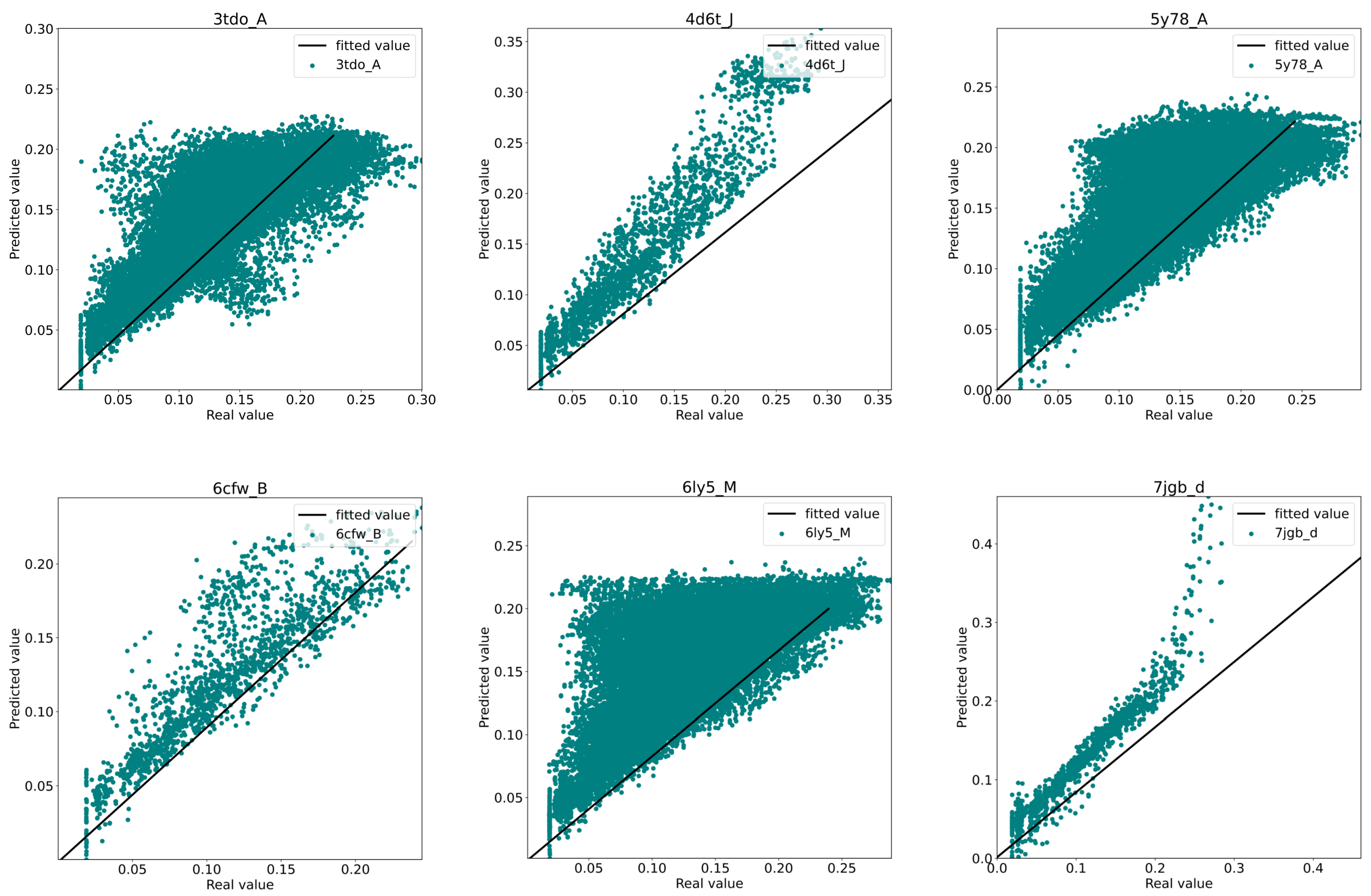
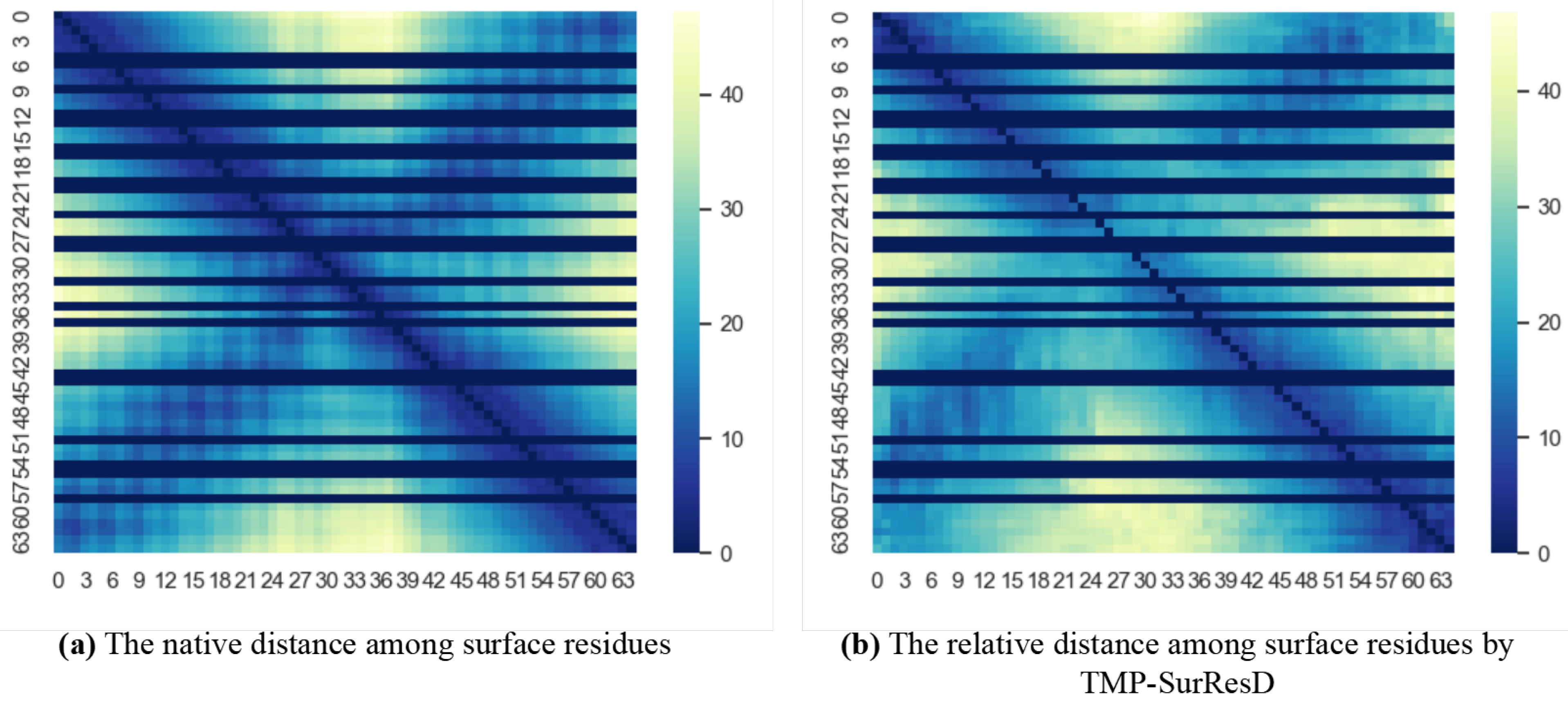
3.3. Model Performance Analysis

After the above parameters tuning, TMP-SurResD ultimately comprises 12 SEB-RB blocks and three layers of FCNN, and the input feature is ‘HHM+CCM’. To verify the stability of TMP-SurResD, we plotted the fitting curve of the model during training, as shown in Figure 3, ensuring that the experimental results are believable and compelling rather than some highly excellent abnormal results. With the continuous advance of the training epoch, the model keeps learning and updating, and the PCC and Loss on the SurTrain and SurValid do not show abnormal changes, indicating that the model designed is relatively stable and can effectively prevent it from falling into local optimum. At the same time, its evaluation indicator changes rapidly and tends to be stable after the end of 40 training epochs. TMP-SurResD converges quickly, saving calculation costs and model training time. In addition, TMP-SurResD does not overfit during the training process and can maintain a very stable state after rapid convergence, ensuring the generalization ability.

A good predictor would not only be highly fit on the training set but should also be able to make correct predictions about unknown data. Therefore, we tested TMP-SurResD on SurTest containing 178 samples to verify the generalization ability and robustness. Especially, SurTest is consistent with the sequence length distribution of the training set and the validation set without any overlap.

Table 5. Performance of TMP-SurResD on TestSur.

Features	MAE	MSE	PCC
CCM	0.0473	0.0054	0.7238
HHM+CCM	0.0504	0.0055	0.6999
OH+HHM+CCM	0.0522	0.0063	0.6878

demonstrates that TMP-SurResD has significantly excellent generalization ability and robustness. When three types of combinations (‘CCM’, ‘HHM+CCM’, and ‘OH+HHM+CCM’) are inputs, the PCC is 0.7238, 0.6999, and 0.6878, respectively. These results indicate that TMP-SurResD has good generalization ability.

3.4. The Setting of Residue-Residue Distances Threshold

Previous studies mainly focused on residue contact [14,15,45,54,55,56,57,58,59,60,61,62,63,64,65,66,67], but the latent structure information is relatively insufficient than the distance among residues. As we all know, residue contacts are often obtained by setting thresholds. Therefore, it is meaningful to explore the results obtained from TMP-SurResD to select the appropriate distance threshold. For 178 test data, we plotted the relationship between the predicted and actual values as shown in Figure 4 (Only six samples are listed here). It can be seen from the figure that the distance of the surface residues predicted is larger than the actual distance. It is reasonable because the relative distance is concerned rather than individual residue pair distance.

Here, we took the chain E of TMP 3DIN as an example of a case study to demonstrate the effectiveness of TMP-SurResD further. 3DIN_E containing 65 residues [68] is an essential part of the protein-translocation complex formed by the SecY channel and the SecA ATPase in Escherichia coli. It could be folded with very high accuracy. Figure 5 compares the TMP-SurResD predicted relative distances and real distances. As shown in the figures, the overall trend of the relative distances has been appropriately captured. However, compared with the true value, the predicted value is generally more significant, which can be easily seen from the color depth in the left and right pictures.

On this basis, we set the distance threshold. As seen from

Table 6. The ability of TMP-SurResD to predict residue contacts by setting different thresholds of predicted values ¹.

Threshold	ACC	Precision	Recall	F1	MCC
5.5	0.9825	0.9055	0.1725	0.2755	0.3667
6	0.9777	0.9434	0.1837	0.2950	0.3887
6.5	0.9737	0.9607	0.1951	0.3128	0.4066
7	0.9725	0.9666	0.2219	0.3483	0.4372
7.5	0.9728	0.9682	0.2658	0.4021	0.4814
8	0.9736	0.9656	0.3221	0.4654	0.5313
8.5	0.9728	0.9619	0.3631	0.5089	0.5651
9	0.9697	0.9620	0.3794	0.5274	0.5788
9.5	0.9684	0.9655	0.4039	0.5534	0.5997
10	0.9645	0.9676	0.4065	0.5576	0.6020
10.5	0.9594	0.9674	0.3973	0.5498	0.5940
11	0.9546	0.9647	0.3895	0.5422	0.5859

¹ Here, classification evaluation metrics such as ACC, Precision, Recall, F1, and MCC are employed to evaluate the residue contact prediction ability of TMP-SurResD.We take 5.5 as the initial value and successively increase the threshold value with the step size of 0.5.

, when the threshold is set to 10, the higher precision is 0.9676, which illustrates that the prediction ability of TMP-SurResD is relatively good. The recall is 0.4065, representing the probability of being correctly predicted in contact residue pairs. F1-score is 0.5576, which is a comprehensive evaluation index to improve precision and recall as much as possible while minimizing the difference between them. The Matthews Correlation Coefficient (MCC) is 0.602, a reliable metric for dichotomies, as the model’s predictive performance is comprehensively considered from true positives, true negatives, false positives, and false negatives. The above results show that when the overall distance between the surface residues is too large, the threshold we set is too high.

3.5. Comparison with Residue Contact Prediction Models

Previous residue contact models utilized the distance threshold 8 to define residue contacts, so eight is also used in our study for a fair comparison.

Table 7. Comparison of TMP-SurResD and other residue contact prediction methods based on surface residue ¹.

Model	ProNum	ACC	Precision	Recall	F1	MCC
PSICOV	128	0.0011	0.9062	0.0011	0.0022	0.0000
Freecontact	178	0.0612	0.9831	0.0612	0.0959	0.0000
DEEPCON	178	0.0024	0.9944	0.0024	0.0047	0.0000
TMP-SurResD	178	0.9736	0.9656	0.3221	0.4654	0.5313

¹ Results of TMP-SurResD with a distance threshold of 8 were compared with other protein residue contact predictors on SurTest. The ’Model’ column lists the various methods used for comparison; the corresponding indicators (ACC, Precision, Recall, F1, and MCC) are taken advantage of to evaluate the predictor; the column ‘ProNum’ denotes the number of protein sequences correctly predicted by these methods.

indicates that TMP-SurResD has an excellent residue contact prediction ability compared with PSICOV [69], Freecontact [60], and DEEPCON [45]. From the perspective of input, the four comparison methods directly utilized MSAs. However, the correct residue contact prediction cannot be made because TMPs need many homologous sequences. Furthermore, from the ’Precision’ and ’Recall’ columns, precision reflects the discrimination ability of the model to negative samples, and recall reveals the identification ability to positive samples. It can be seen from the results that all predictors can correctly judge negative samples in surface residue pairs. Nevertheless, TMP-SurResD can accurately determine the positive samples, although recall is only 0.3221. The F1 score of 0.4654 indicates that TMP-SurResD is relatively stable. To summarize, the residue contact obtained by setting an appropriate threshold is superior to other comparison methods.

4. Discussion

Interactions between amino acid residues on polypeptide chains and surrounding media play a decisive role in stable tertiary structure folding. From a macro perspective, the spatial protein structure shows that multiple residues are very close to each other in space through interaction forces. Accurate knowledge of the spatial distance between pairs of residues can add more constraints to guide high-quality protein structure prediction. Studies have shown that surface residues directly related to function and structure can assist in obtaining the high-quality tertiary structure of proteins. We focused on predicting TMP residue distance using the deep learning method successfully applied to hydro-soluble protein residue contact prediction. Furthermore, the deep learning model, TMP-SurResD, was proposed to fill the research gap and provide references for future research.

In the absence of sufficient TMP training samples to fit the weight parameters, it is not optimal to simultaneously use all the features as inputs to the model. The combination of coevolution and evolutionary conservation played a crucial role in predicting surface residue distance and transmembrane residue distance. The results demonstrated that our proposed model showed good robustness and generalization ability in both training and test sets. It performed better than other water-soluble protein classification models in classification evaluation indexes.

At the same time, we found some shortcomings. Currently, the number of known TMP structures is limited, and many TMP sequences still need help finding sufficient homology information to generate co-evolutionary characteristics. When little information about an unknown protein structure is known, or the homologous sequence of the target protein cannot be found, the accuracy of residue distance prediction is relatively low, and even the auxiliary protein structure prediction has the opposite effect. TMP-SurResD still fails to predict TMPs accurately with the short homologous sequences. Therefore, how to achieve the end-to-end prediction of sequence to structure without using any homologous sequence information and other complex manual features is still an urgent problem to be solved.

References

1. Qu, J.; Yin, S.S.; Wang, H. Prediction of Metal Ion Binding Sites of Transmembrane Proteins. Comput. Math. Methods Med. 2021, 2021, 2327832. [Google Scholar] [CrossRef] [PubMed]
2. Yin, H.; Flynn, A.D. Drugging Membrane Protein Interactions. Annu. Rev. Biomed. Eng. 2016, 18, 51–76. [Google Scholar] [CrossRef] [PubMed] [Green Version]
3. Zaucha, J.; Heinzinger, M.; Kulandaisamy, A.; Kataka, E.; Salvádor, L.; Popov, P.; Rost, B.; Gromiha, M.M.; Zhorov, B.S.; Frishman, D. Mutations in transmembrane proteins: Diseases, evolutionary insights, prediction and comparison with globular proteins. Briefings Bioinform. 2021, 22, bbaa132. [Google Scholar] [CrossRef] [PubMed]
4. Mashayekhi, V.; Mocellin, O.; Fens, M.H.A.M.; Krijger, G.C.; Brosens, L.A.A.; Oliveira, S. Targeting of promising transmembrane proteins for diagnosis and treatment of pancreatic ductal adenocarcinoma. Theranostics 2021, 11, 9022–9037. [Google Scholar] [CrossRef]
5. Liu, Z.; Gong, Y.; Guo, Y.; Zhang, X.; Lu, C.; Zhang, L.; Wang, H. TMP- SSurface2: A Novel Deep Learning-Based Surface Accessibility Predictor for Transmembrane Protein Sequence. Front. Genet. 2021, 12, 656140. [Google Scholar] [CrossRef]
6. Lu, C.; Liu, Z.; Zhang, E.; He, F.; Ma, Z.; Wang, H. MPLs-Pred: Predicting Membrane Protein-Ligand Binding Sites Using Hybrid Sequence-Based Features and Ligand-Specific Models. Int. J. Mol. Sci. 2019, 20, 3120. [Google Scholar] [CrossRef] [Green Version]
7. Kovalenko, O.; Metcalf, D.; DeGrado, W.; Hemler, M. Structural organization and interactions of transmembrane domains in tetraspanin proteins. BMC Struct. Biol. 2005, 5, 11. [Google Scholar] [CrossRef] [Green Version]
8. Wang, S.; Sun, S.; Li, Z.; Zhang, R.; Xu, J. Accurate De Novo Prediction of Protein Contact Map by Ultra-Deep Learning Model. PLoS Comput. Biol. 2016, 13, e1005324. [Google Scholar] [CrossRef] [Green Version]
9. Zhang, H.; Huang, Y.; Bei, Z.; Ju, Z.; Meng, J.; Hao, M.; Zhang, J.; Zhang, H.; Xi, W. Inter-Residue Distance Prediction from Duet Deep Learning Models. Front. Genet. 2022, 13, 887491. [Google Scholar] [CrossRef]
10. Zhang, J.; Zhang, Y.; Ma, Z. In silico Prediction of Human Secretory Proteins in Plasma Based on Discrete Firefly Optimization and Application to Cancer Biomarkers Identification. Front. Genet. 2019, 10, 542. [Google Scholar] [CrossRef] [Green Version]
11. Rose, P.W.; Beran, B.; Bi, C.; Bluhm, W.; Dimitropoulos, D.; Goodsell, D.S.; Prlić, A.; Quesada, M.; Quinn, G.B.; Westbrook, J.D.; et al. The RCSB Protein Data Bank: Redesigned web site and web services. Nucleic Acids Res. 2011, 39, D392–D401. [Google Scholar] [CrossRef] [PubMed] [Green Version]
12. Wang, H.; Yang, Y.; Yu, J.; Wang, X.; Zhao, D.; Xu, D.; Sun, P. DMCTOP: Topology Prediction of Alpha-Helical Transmembrane Protein Based on Deep Multi-Scale Convolutional Neural Network. In Proceedings of the 2019 IEEE International Conference on Bioinformatics and Biomedicine (BIBM), San Diego, CA, USA, 18–21 November 2019; pp. 36–43. [Google Scholar]
13. Tunyasuvunakool, K.; Adler, J.; Wu, Z.; Green, T.; Zielinski, M.; Zídek, A.; Bridgland, A.; Cowie, A.; Meyer, C.; Laydon, A.; et al. Highly accurate protein structure prediction for the human proteome. Nature 2021, 596, 590–596. [Google Scholar] [CrossRef] [PubMed]
14. Hönigschmid, P.; Frishman, D. Accurate prediction of helix interactions and residue contacts in membrane proteins. J. Struct. Biol. 2016, 194, 112–123. [Google Scholar] [CrossRef] [PubMed] [Green Version]
15. Yang, J.; Shen, H.B. MemBrain-contact 2.0: A new two-stage machine learning model for the prediction enhancement of transmembrane protein residue contacts in the full chain. Bioinformatics 2018, 34, 230–238. [Google Scholar] [CrossRef] [PubMed] [Green Version]
16. Ji, S.; Oruç, T.; Mead, L.; Rehman, M.F.; Thomas, C.M.; Butterworth, S.; Winn, P.J. DeepCDpred: Inter-residue distance and contact prediction for improved prediction of protein structure. PLoS ONE 2019, 14, e0205214. [Google Scholar] [CrossRef] [Green Version]
17. Ding, W.; Gong, H. Predicting the Real-Valued Inter-Residue Distances for Proteins. Adv. Sci. 2020, 7, 2001314. [Google Scholar] [CrossRef]
18. Du, Z.; Peng, Z.; Yang, J. Toward the assessment of predicted inter-residue distance. Bioinformatics 2022, 38, 962–969. [Google Scholar] [CrossRef]
19. Wu, T.; Guo, Z.; Hou, J.; Cheng, J. DeepDist: Real-value inter-residue distance prediction with deep residual convolutional network. BMC Bioinform. 2020, 22, 30. [Google Scholar]
20. Kuhlman, B.; Bradley, P. Advances in protein structure prediction and design. Nat. Rev. Mol. Cell Biol. 2019, 20, 681–697. [Google Scholar] [CrossRef] [PubMed]
21. Senior, A.W.; Evans, R.; Jumper, J.M.; Kirkpatrick, J.; Sifre, L.; Green, T.; Qin, C.; Zídek, A.; Nelson, A.W.R.; Bridgland, A.; et al. Improved protein structure prediction using potentials from deep learning. Nature 2020, 577, 706–710. [Google Scholar] [CrossRef]
22. Ju, F.; Zhu, J.; Shao, B.; Kong, L.; Liu, T.Y.; Zheng, W.; Bu, D. CopulaNet: Learning residue co-evolution directly from multiple sequence alignment for protein structure prediction. Nat. Commun. 2020, 12, 2535. [Google Scholar] [CrossRef]
23. Russakovsky, O.; Deng, J.; Su, H.; Krause, J.; Satheesh, S.; Ma, S.; Huang, Z.; Karpathy, A.; Khosla, A.; Bernstein, M.S.; et al. ImageNet Large Scale Visual Recognition Challenge. Int. J. Comput. Vis. 2015, 115, 211–252. [Google Scholar] [CrossRef] [Green Version]
24. Hu, J.; Shen, L.; Sun, G. Squeeze-and-Excitation Networks. In Proceedings of the 2018 IEEE/CVF Conference on Computer Vision and Pattern Recognition, Salt Lake City, UT, USA, 18–22 June 2018; pp. 7132–7141. [Google Scholar]
25. Kozma, D.; Simon, I.; Tusnády, G.E. PDBTM: Protein Data Bank of transmembrane proteins after 8 years. Nucleic Acids Res. 2013, 41, D524–D529. [Google Scholar] [CrossRef] [Green Version]
26. Huang, Y.; Niu, B.; Gao, Y.; Fu, L.; Li, W. CD-HIT Suite: A web server for clustering and comparing biological sequences. Bioinformatics 2010, 26, 680–682. [Google Scholar] [CrossRef] [PubMed]
27. Luo, F.; Wang, M.; Liu, Y.; Zhao, X.; Li, A. DeepPhos: Prediction of protein phosphorylation sites with deep learning. Bioinformatics 2019, 35, 2766–2773. [Google Scholar] [CrossRef] [PubMed] [Green Version]
28. Kawashima, S.; Ogata, H.; Kanehisa, M. AAindex: Amino Acid Index Database. Nucleic Acids Res. 1999, 27, 368–369. [Google Scholar] [CrossRef] [PubMed] [Green Version]
29. Shen, H.; Chou, K.C. PseAAC: A flexible web server for generating various kinds of protein pseudo amino acid composition. Anal. Biochem. 2008, 373, 386–388. [Google Scholar] [CrossRef] [PubMed]
30. Liu, Z.; Gong, Y.; Bao, Y.; Guo, Y.; Wang, H.; Lin, G.N. TMPSS: A Deep Learning-Based Predictor for Secondary Structure and Topology Structure Prediction of Alpha-Helical Transmembrane Proteins. Front. Bioeng. Biotechnol. 2020, 8, 629937. [Google Scholar] [CrossRef]
31. Lim, S.; Lu, Y.; Cho, C.Y.; Sung, I.; Kim, J.; Kim, Y.; Park, S.; Kim, S. A review on compound-protein interaction prediction methods: Data, format, representation and model. Comput. Struct. Biotechnol. J. 2021, 19, 1541–1556. [Google Scholar] [CrossRef]
32. Ding, H.; Li, D. Identification of mitochondrial proteins of malaria parasite using analysis of variance. Amino Acids 2015, 47, 329–333. [Google Scholar] [CrossRef]
33. ElAbd, H.; Bromberg, Y.; Hoarfrost, A.; Lenz, T.L.; Franke, A.; Wendorff, M. Amino acid encoding for deep learning applications. BMC Bioinform. 2020, 21, 235. [Google Scholar] [CrossRef]
34. Zeng, B.; Hönigschmid, P.; Frishman, D. Residue co-evolution helps predict interaction sites in α-helical membrane proteins. J. Struct. Biol. 2019, 206 2, 156–169. [Google Scholar] [CrossRef]
35. Remmert, M.; Biegert, A.; Hauser, A.; Söding, J. HHblits: Lightning-fast iterative protein sequence searching by HMM-HMM alignment. Nat. Methods 2012, 9, 173–175. [Google Scholar] [CrossRef] [PubMed]
36. Zhang, C.; Zheng, W.; Mortuza, S.M.; Li, Y.; Zhang, Y. DeepMSA: Constructing deep multiple sequence alignment to improve contact prediction and fold-recognition for distant-homology proteins. Bioinformatics 2020, 36, 2105–2112. [Google Scholar] [CrossRef] [PubMed]
37. de Juan, D.; Pazos, F.; Valencia, A. Emerging methods in protein co-evolution. Nat. Reviews. Genet. 2013, 14, 249–261. [Google Scholar] [CrossRef]
38. Seemayer, S.; Gruber, M.; Söding, J. CCMpred—Fast and precise prediction of protein residue–residue contacts from correlated mutations. Bioinformatics 2014, 30, 3128–3130. [Google Scholar] [CrossRef] [PubMed] [Green Version]
39. Haldane, A.; Levy, R.M. Influence of multiple-sequence-alignment depth on Potts statistical models of protein covariation. Phys. Rev. E 2019, 99, 032405. [Google Scholar] [CrossRef] [PubMed]
40. Ma, J.; Wang, S. AcconPred: Predicting Solvent Accessibility and Contact Number Simultaneously by a Multitask Learning Framework under the Conditional Neural Fields Model. BioMed Res. Int. 2015, 2015, 678764. [Google Scholar] [CrossRef] [Green Version]
41. Jeong, J.C.; Lin, X.; Chen, X.W. On Position-Specific Scoring Matrix for Protein Function Prediction. IEEE/ACM Trans. Comput. Biol. Bioinform. 2011, 8, 308–315. [Google Scholar] [CrossRef]
42. Eigen, D.; Puhrsch, C.; Fergus, R. Depth Map Prediction from a Single Image using a Multi-Scale Deep Network. In Advances in Neural Information Processing Systems 27 (NIPS 2014); MIT Press: Cambridge, MA, USA, 2014; pp. 2366–2374. [Google Scholar]
43. Laina, I.; Rupprecht, C.; Belagiannis, V.; Tombari, F.; Navab, N. Deeper Depth Prediction with Fully Convolutional Residual Networks. In Proceedings of the 2016 Fourth International Conference on 3D Vision (3DV), Stanford, CA, USA, 25–28 October 2016; pp. 239–248. [Google Scholar]
44. Chen, S.; Tang, M.; Kan, J. Monocular image depth prediction without depth sensors: An unsupervised learning method. Appl. Soft Comput. 2020, 97, 106804. [Google Scholar] [CrossRef]
45. Adhikari, B. DEEPCON: Protein Contact Prediction using Dilated Convolutional Neural Networks with Dropout. bioRxiv 2019. [Google Scholar] [CrossRef]
46. Jones, D.T.; Kandathil, S.M. High precision in protein contact prediction using fully convolutional neural networks and minimal sequence features. Bioinformatics 2018, 34, 3308–3315. [Google Scholar] [CrossRef] [PubMed] [Green Version]
47. Nair, V.; Hinton, G.E. Rectified Linear Units Improve Restricted Boltzmann Machines. In Proceedings of the International Conference on Machine Learning, Haifa, Israel, 21–24 June 2010. [Google Scholar]
48. He, K.; Zhang, X.; Ren, S.; Sun, J. Deep Residual Learning for Image Recognition. In Proceedings of the 2016 IEEE Conference on Computer Vision and Pattern Recognition (CVPR), Santiago, Chile, 26 June–1 July 2016; pp. 770–778. [Google Scholar]
49. Paszke, A.; Gross, S.; Massa, F.; Lerer, A.; Bradbury, J.; Chanan, G.; Killeen, T.; Lin, Z.; Gimelshein, N.; Antiga, L.; et al. PyTorch: An Imperative Style, High-Performance Deep Learning Library. arXiv 2019, arXiv:1912.01703. [Google Scholar]
50. Kingma, D.P.; Ba, J. Adam: A Method for Stochastic Optimization. arXiv 2015, arXiv:1412.6980. [Google Scholar]
51. DeGhett, V.J. Effective use of Pearson’s product-moment correlation coefficient: An additional point. Anim. Behav. 2014, 98, e1–e2. [Google Scholar] [CrossRef]
52. Gromiha, M.M.; Selvaraj, S. Inter-residue interactions in protein folding and stability. Prog. Biophys. Mol. Biol. 2004, 86, 235–277. [Google Scholar] [CrossRef] [PubMed]
53. Zhang, C.; Kim, S. Environment-dependent residue contact energies for proteins. Proc. Natl. Acad. Sci. USA 2000, 97, 2550–2555. [Google Scholar] [CrossRef] [Green Version]
54. Latek, D.; Kolinski, A. Contact prediction in protein modeling: Scoring, folding and refinement of coarse-grained models. BMC Struct. Biol. 2008, 8, 36. [Google Scholar] [CrossRef] [Green Version]
55. Lo, A.; Chiu, Y.Y.; Rødland, E.A.; Lyu, P.C.; Sung, T.Y.; Hsu, W.L. Predicting helix–helix interactions from residue contacts in membrane proteins. Bioinformatics 2009, 25, 996–1003. [Google Scholar] [CrossRef] [Green Version]
56. Morcos, F.; Pagnani, A.; Lunt, B.; Bertolino, A.; Marks, D.S.; Sander, C.; Zecchina, R.; Onuchic, J.N.; Hwa, T.; Weigt, M. Direct-coupling analysis of residue coevolution captures native contacts across many protein families. Proc. Natl. Acad. Sci. USA 2011, 108, E1293–E1301. [Google Scholar] [CrossRef] [Green Version]
57. Kamisetty, H.; Ovchinnikov, S.; Baker, D. Assessing the utility of coevolution-based residue–residue contact predictions in a sequence- and structure-rich era. Proc. Natl. Acad. Sci. USA 2013, 110, 15674–15679. [Google Scholar] [CrossRef] [PubMed] [Green Version]
58. Yang, J.; Jang, R.; Zhang, Y.; Shen, H. High-accuracy prediction of transmembrane inter-helix contacts and application to GPCR 3D structure modeling. Bioinformatics 2013, 29 20, 2579–2587. [Google Scholar] [CrossRef] [Green Version]
59. Jones, D.T.; Singh, T.; Kosciólek, T.; Tetchner, S.J. MetaPSICOV: Combining coevolution methods for accurate prediction of contacts and long range hydrogen bonding in proteins. Bioinformatics 2014, 31, 999–1006. [Google Scholar] [CrossRef] [PubMed] [Green Version]
60. Kaján, L.; Hopf, T.A.; Kalaš, M.; Marks, D.S.; Rost, B. FreeContact: Fast and free software for protein contact prediction from residue co-evolution. BMC Bioinform. 2014, 15, 85. [Google Scholar] [CrossRef] [PubMed] [Green Version]
61. Zhang, H.; Huang, Q.; Bei, Z.; Wei, Y.; Floudas, C.A. COMSAT: Residue contact prediction of transmembrane proteins based on support vector machines and mixed integer linear programming. Proteins Struct. Funct. Bioinform. 2016, 84, 332–348. [Google Scholar] [CrossRef] [PubMed]
62. Yang, J.; Jin, Q.Y.; Zhang, B.; Shen, H. R2C: Improving ab initio residue contact map prediction using dynamic fusion strategy and Gaussian noise filter. Bioinformatics 2016, 32 16, 2435–2443. [Google Scholar] [CrossRef]
63. Hanson, J.; Paliwal, K.K.; Litfin, T.; Yang, Y.; Zhou, Y. Accurate prediction of protein contact maps by coupling residual two-dimensional bidirectional long short-term memory with convolutional neural networks. Bioinformatics 2018, 34, 4039–4045. [Google Scholar] [CrossRef]
64. Fang, C.; Jia, Y.; Hu, L.; Lu, Y.; Wang, H. IMPContact: An Interhelical Residue Contact Prediction Method. BioMed Res. Int. 2020, 2020, 4569037. [Google Scholar] [CrossRef] [Green Version]
65. Sun, J.; Frishman, D. DeepHelicon: Accurate prediction of inter-helical residue contacts in transmembrane proteins by residual neural networks. J. Struct. Biol. 2020, 212, 107574. [Google Scholar] [CrossRef]
66. Li, Y.; Hu, J.; Zhang, C.; Yu, D.J.; Zhang, Y. ResPRE: High-accuracy protein contact prediction by coupling precision matrix with deep residual neural networks. Bioinformatics 2019, 35, 4647–4655. [Google Scholar] [CrossRef]
67. Zhang, H.; Bei, Z.; Xi, W.; Hao, M.; Ju, Z.; Saravanan, K.M.; Zhang, H.; Guo, N.; Wei, Y. Evaluation of residue-residue contact prediction methods: From retrospective to prospective. PLoS Comput. Biol. 2021, 17, e1009027. [Google Scholar] [CrossRef] [PubMed]
68. Zimmer, J.; Nam, Y.; Rapoport, T.A. Structure of a complex of the ATPase SecA and the protein-translocation channel. Nature 2008, 455, 936–943. [Google Scholar] [CrossRef] [PubMed]
69. Jones, D.T.; Buchan, D.W.A.; Cozzetto, D.; Pontil, M. PSICOV: Precise structural contact prediction using sparse inverse covariance estimation on large multiple sequence alignments. Bioinformatics 2012, 28, 184–190. [Google Scholar] [CrossRef] [PubMed] [Green Version]
Figure 1. The workflow and architecture of TMP-SurResD.
Mathematics 11 00642 g001
Figure 2. Details of the TMP-SurResD framework. (a) The network used by TMP-SurResD. The feature vectors are L × L × N propagated through 12 SEB-RB blocks and a fully convolutional neural network. In the last output, the matrix of L × L corresponds to the predicted distance between all surface residues; (b) Basic block (SEB-RB) used in the network. (c) Model training process.
Mathematics 11 00642 g002
Figure 3. The changes of Loss, MAE, and PCC on SurTrain and SurValid, respectively.
Mathematics 11 00642 g003
Figure 4. The relationship between the predicted value obtained by TMP-SurResD and the surface residue distance value calculated by coordinates. The black line indicates the fit between the true value and the predicted value; the green scatter demonstrates that the predicted value is larger than the true value.
Mathematics 11 00642 g004
Figure 5. The prediction of TMP-SurResD on a TMP (PDB ID: 3DIN, chain E). Comparison of the native distance map (a) and the predicted distance map by TMP-SurResD (b). The horizontal and vertical coordinates indicate the number of residues, and the darker the color, the closer the residues are. Especially the dark horizontal bars in the figure indicate non-surface residues that are not interesting.
Mathematics 11 00642 g005