
Evaluating the Performance of Synthetic Double Sampling np Chart Based on Expected Median Run Length
 , and
, and
Abstract
:1. Introduction
2. The Review of SDS np Chart
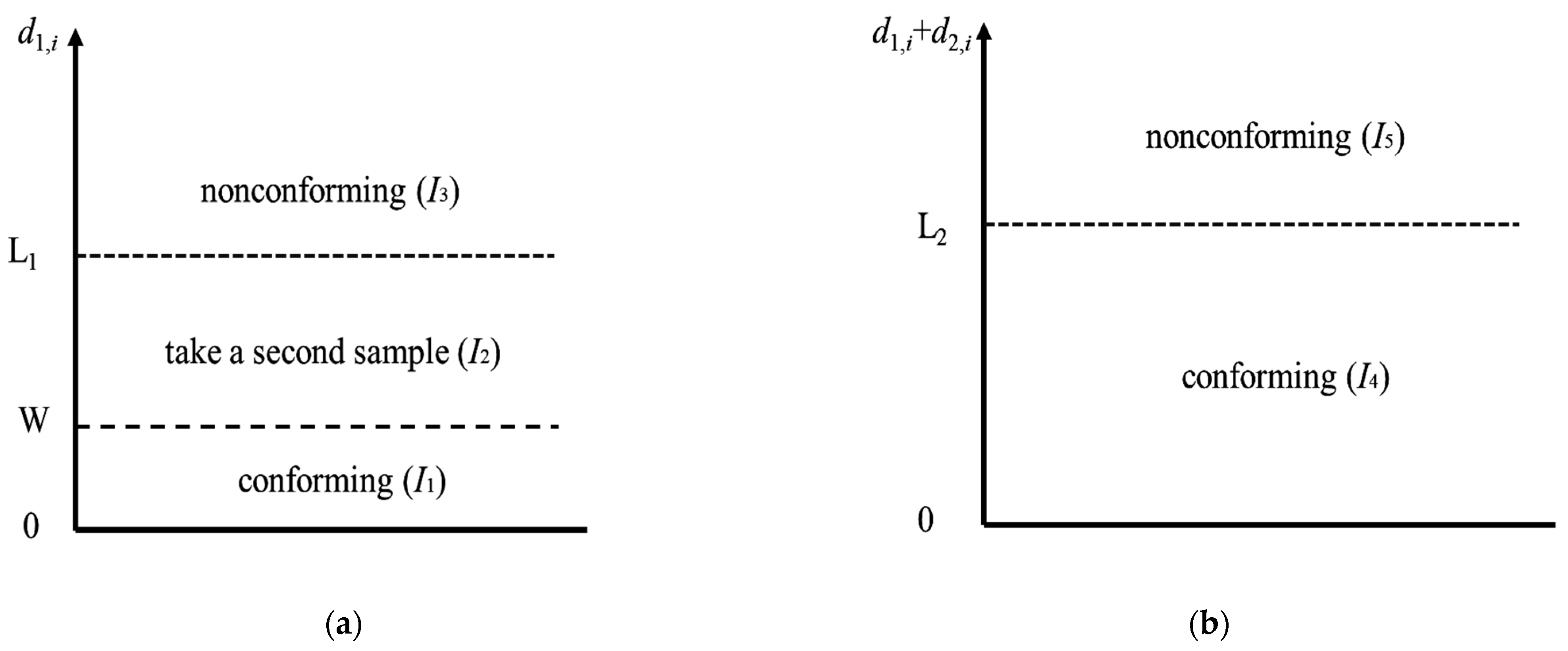
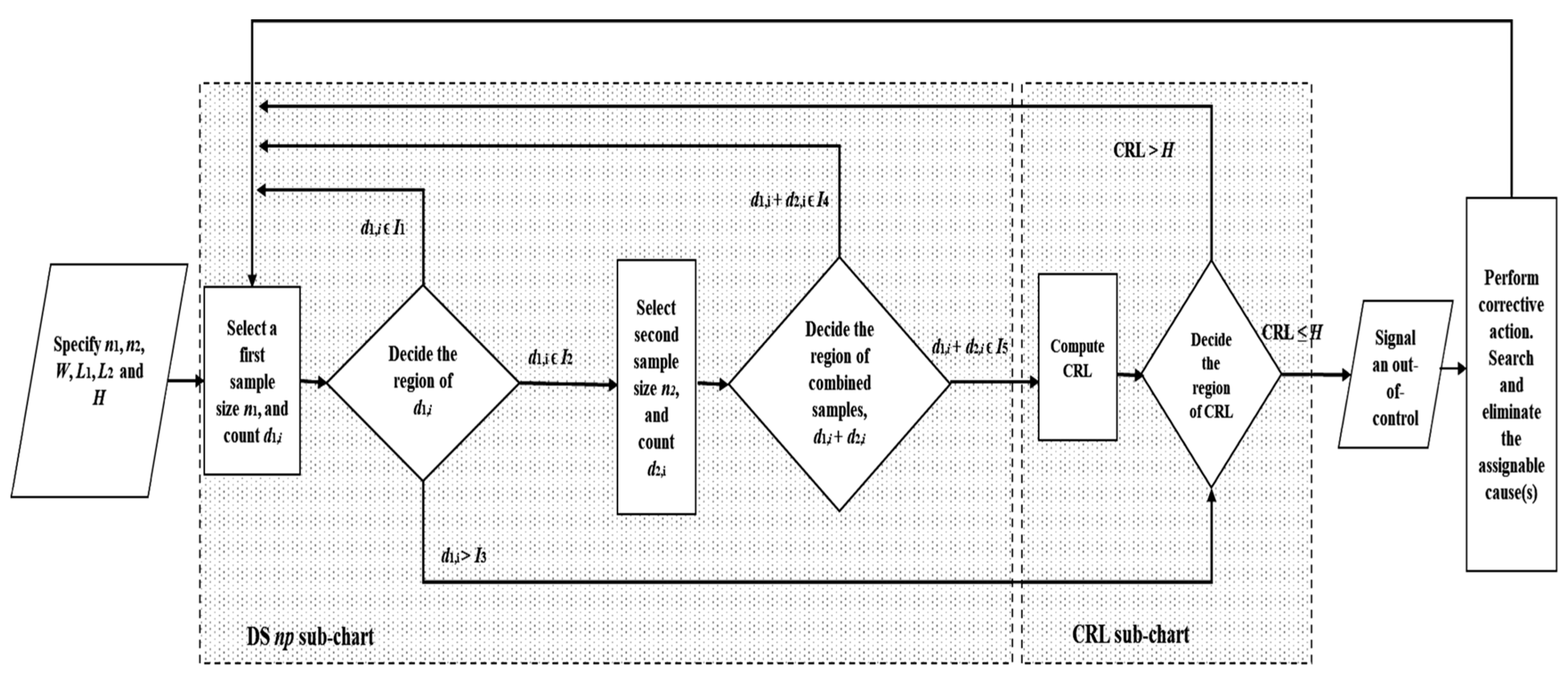
- Step 1:
- Set the optimal charting parameters W, L1, L2 (on DS sub-chart) and H (on CRL sub-chart).
- Step 2:
- Consider the first sample of size n1 and count the number of nonconforming items d1 in the sample.
- Step 3:
- (i)
- If d1,i ϵ I1, the ith sampling stage is categorized as conforming. Process returns to Step 2.
- (ii)
- If d1,i ϵ I3, the ith sampling stage is categorized as nonconforming and control flow advances to Step 5.
- (iii)
- If d1,i ϵ I2, the procedure moves to the second stage of the DS sub-chart. A second sample of size n2 is taken and the number of nonconforming items d2 in the sample is counted. After that, proceed to the next step.
- Step 4:
- Compute the number of nonconforming items in combined samples d1,i + d2,i. If (d1,i + d2,i) ϵ I4, the ith sampling stage is categorized as conforming and the control flow returns to Step 2. If this is not the case, the sampling stage is categorized as nonconforming, and the control flow moves to Step 5.
- Step 5:
- Count the number of sampling stages, including the current nonconforming sampling stage, that separate two successive nonconforming sampling stages and is known as CRL value.
- Step 6:
- If CRL > H, the process is deemed as IC and the control flow goes back to Step 2. Otherwise, the process is judged as OOC and corrective action is required to search and eliminate the assignable cause(s). Then, the process goes back to Step 2.
3. The Run Length Properties of the SDS np Chart
4. Optimization Designs Procedure
4.1. Computation of the Optimal Charting Parameter for the SDS np Chart to Minimize MRL1
- Step 1:
- Specify the p0, n, MRL0min and values. Here, n is the average sample size at every sampling stage when the process is in an IC state.
- Step 2:
- Set H to one at the start.
- Step 3:
- Set the initial value of MRL1min to 105 (a relatively large value).
- Step 4:
- Start with n1 equal to one.
- Step 5:
- With the current n1 value, the combination of (n1, n2, W, L1, H) is determined for a specified n when , such that the Constraint (19) is fulfilled. The value of n2 is obtained by rearranging Equation (13), i.e., , and is rounded up to the nearest integer, where 0 < W < L1.
- Step 6:
- For the ZS mode, L2 is determined via Constraint (18) together with Equations (5) and (10). For the SS mode, on the other hand, L2 can be obtained by solving Constraint (18) together with Equations (6) and (10). The computed MRL equals to MRL0 when (i.e., p = p0), where L2 > L1. In this step, the possible (n1, n2, W, L1, L2, H) combination is identified.
- Step 7:
- Once the possible (n1, n2, W, L1, L2, H) combination is determined, MRL1 will be computed for p = p1, by means of Equations (5) and (10) (for ZS mode) or Equations (6) and (10) (for SS mode). If the computed MRL1 is less than the present MRL1min, substitute the newly computed MRL1 for the MRL1min value. The (n1, n2, W, L1, L2, H) combination is saved temporarily as the possible combination. If the (n1, n2, W, L1, L2, H) combination found in the following searching produces identical MRL1min, it will be kept together as a possible combination. Otherwise, if the (n1, n2, W, L1, L2, H) combination results in a larger MRL1 value, it will be ignored.
- Step 8:
- Once the search with n1 = 1 is complete, n1 is increased by one. Repeat Steps 5–7 for each remaining n1 = 2, 3…, (), in order to find the possible (n1, n2, W, L1, L2, H) combinations that fulfil the Constraints (18) and (19) and having the lowest value of MRL1.
- Step 9:
- If MRL1min value has been reduced, increase H by 1 and repeat Steps 3–8. Else, proceed to Step 10.
- Step 10:
- If more than one combination of (n1, n2, W, L1, L2, H) delivers a similar minimum MRL1min value, the combination that produces the smallest OOC average sample size (ASS1) value is chosen as the optimal combination. Additionally, if more than one combination of (n1, n2, W, L1, L2, H) produces similar comparable lowest pair values (MRL1, ASS1), the parameters combination corresponding to the lowest H is taken to be the optimal combination in this case.
4.2. Computation of the Optimal Charting Parameter for the SDS np Chart to Minimize EMRL1
- Step 1:
- Specify the desired values of , , n, p0, and .
- Step 2:
- Similar to Steps 2 to 5 of the optimization procedure outlined in Section 5.1, but ↓ with
- Step 3:
- Constraints (21) and (22) in place of Constraints (18) and (19) by minimizing the OOC EMRL (EMRL1) in Equation (20).
- Step 4:
- For the ZS mode, L2 is based on the Equations (5) and (10) and Constraint (21), in which the computed EMRL equals to EMRL0 (i.e., when p = p0), where . Note that for the case of SS mode, on the other hand, L2 can be obtained by solving Constraint (21) together with Equations (6) and (10). The non-integer setting of W, L1 and L2 are based on operating procedure of DS sub-chart as described in Section 2. In this step, the possible parameters (n1, n2, W, L1, L2, H) combination is identified.
- Step 5:
- Once the possible (n1, n2, W, L1, L2, H) combination has been identified, EMRL1 is calculated (i.e., when p = p1), by means of Equations (5), (10) and (14) (for ZS mode) or Equations (6), (10) and (14) (for SS mode). If the calculated EMRL1 is lower than the present EMRL1min, substitute the newly computed EMRL1 for the EMRL1min value. The current (n1, n2, W, L1, L2, H) combination is temporarily saved as the possible combination. If the combination (n1, n2, W, L1, L2, H) obtained in the subsequent searching produces an EMRL1min that is comparable to the one being searched for, the combination will be saved as a possible one. If this is not the case, the combination (n1, n2, W, L1, L2, H) will be disregarded if the EMRL1 value that it produces is higher.
- Step 6:
- Increase n1 by one when the search is finished with n1 = 1. For the remaining n1 = 2, 3…, (), repeat Steps 5 through 7, to look for the possible (n1, n2, W, L1, L2, H) combinations that fulfil Constraints (21)–(22) and have the lowest value of EMRL1.
- Step 7:
- If the EMRL1min value has been lowered, raise H by 1 and repeat Steps 3–8. Otherwise, move on to Step 10.
- Step 8:
- If multiple combinations of (n1, n2, W, L1, L2, H) give a similar minimum EMRL1min value, the optimal combination is the one that produces the lowest OOC expected average sample size (EASS1) value. Additionally, if more than one combination of (n1, n2, W, L1, L2, H) produces a similar comparable lowest pair (EMRL1, EASS1) value, the parameter combination corresponding to the lowest H is taken to be the optimal combination in this case.
5. Comparative Studies
5.1. Performance Analysis of the SDS np Chart Based on MRL
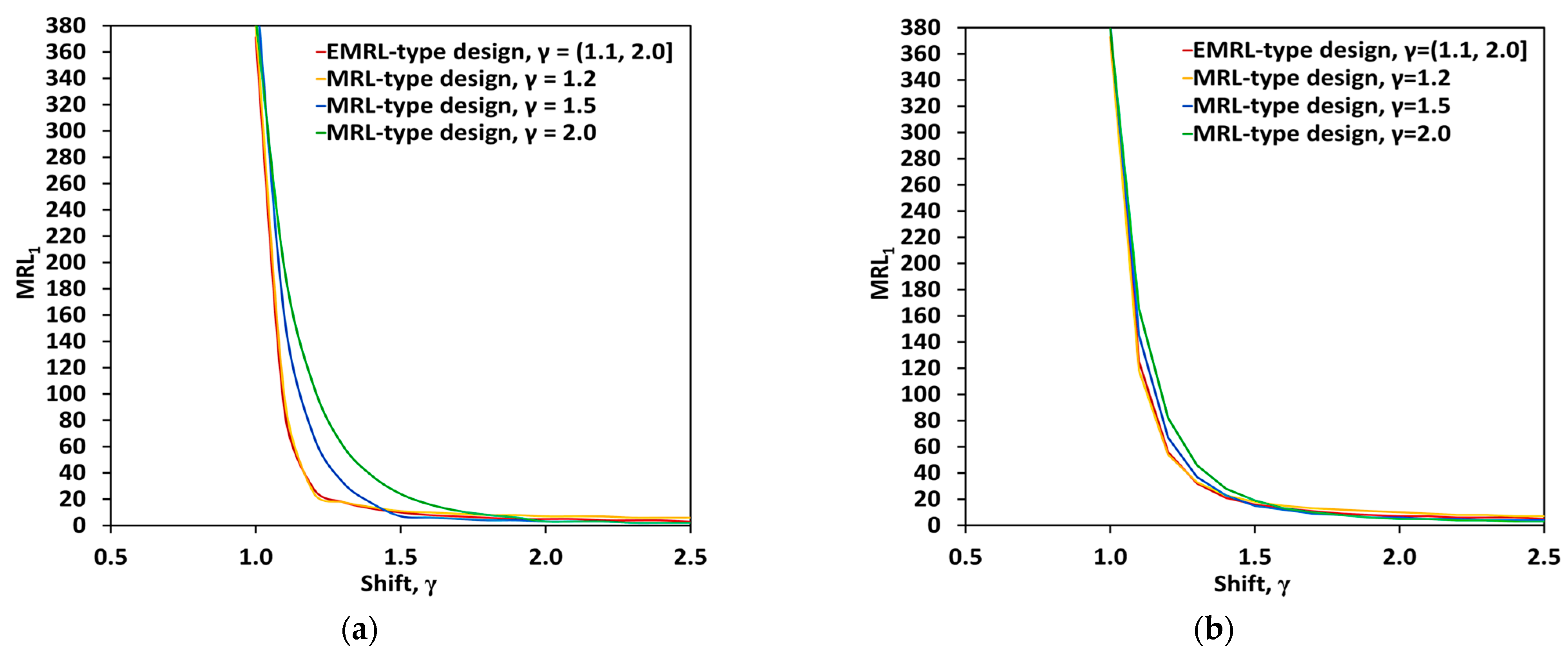
5.2. Performance Analysis of the SDS np Chart Based on EMRL
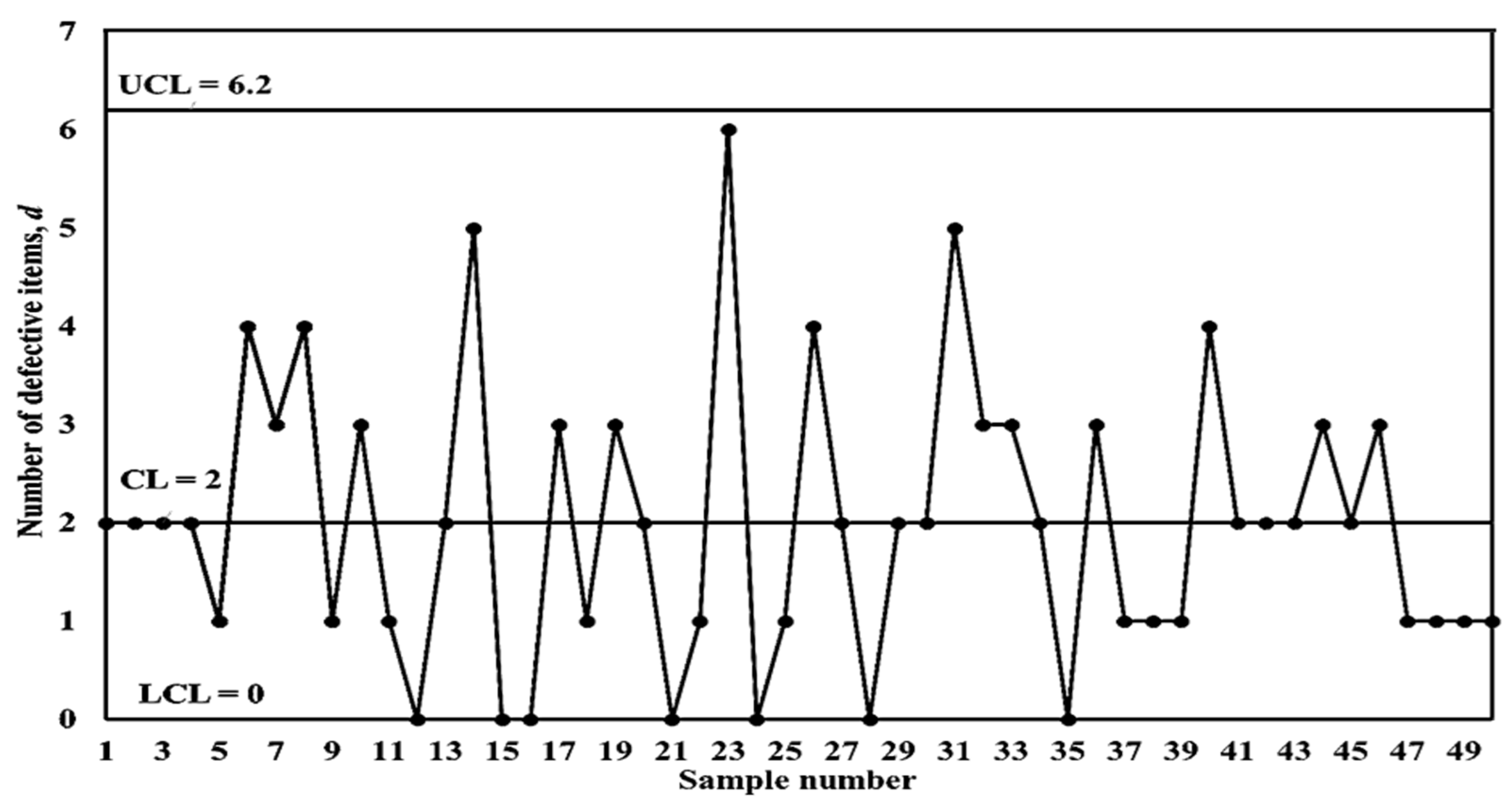
6. An Illustrative Example
7. Conclusions
Author Contributions
Funding
Institutional Review Board Statement
Informed Consent Statement
Data Availability Statement
Acknowledgments
Conflicts of Interest
References
- Khoo, M.B.C.; Lee, H.C.; Wu, Z.; Chen, C.H.; Castagliola, P. A synthetic double sampling control chart for the process mean. IIE Trans. 2010, 43, 23–38. [Google Scholar] [CrossRef]
- Khoo, M.B.C.; Wu, Z.; Castagliola, P.; Lee, H.C. A multivariate synthetic double sampling T2 control chart. Comput. Ind. Eng. 2013, 64, 179–189. [Google Scholar] [CrossRef]
- Bourke, P.D. Detecting a shift in fraction nonconforming using run-length control charts with 100% inspection. J. Qual. Technol. 1991, 23, 225–238. [Google Scholar] [CrossRef]
- Lee, M.H.; Khoo, M.B.C. Synthetic double sampling s chart. Commun. Stat.-Theory Methods 2017, 46, 5914–5931. [Google Scholar] [CrossRef]
- Costa, A.F.B.; Machado, M.A.G. The steady-state behavior of the synthetic and side-sensitive synthetic double sampling charts. Qual. Reliab. Eng. Int. 2015, 31, 297–303. [Google Scholar] [CrossRef]
- Haq, A.; Khoo, M.B.C. A synthetic double sampling control chart for process mean using auxiliary information. Qual. Reliab. Eng. Int. 2019, 35, 1803–1825. [Google Scholar] [CrossRef]
- You, H.W.; Khoo, M.B.C.; Lee, M.H.; Castagliola, P. Synthetic double sampling chart with estimated process parameters. Qual. Technol. Quant. Manag. 2015, 12, 579–604. [Google Scholar] [CrossRef]
- You, H.W. Performance of synthetic double sampling chart with estimated parameters based on expected average run length. J. Probab. Stat. 2018, 2018, 7583610. [Google Scholar] [CrossRef] [Green Version]
- Lorenzen, T.J.; Vance, L.C. The economic design of control charts: A unified approach. Technometrics 1986, 28, 3–10. [Google Scholar] [CrossRef]
- Lee, M.H.; Khoo, M.B.C. Economic-statistical design of synthetic double sampling T2 chart. Commun. Stat.-Theory Methods 2019, 48, 5862–5876. [Google Scholar] [CrossRef]
- Lee, M.H.; Khoo, M.B.C. The economic and economic statistical designs of synthetic double sampling chart. Commun. Stat.-Simul. Comput. 2019, 48, 2313–2332. [Google Scholar] [CrossRef]
- Aghaulor, C.D.; Ezekwem, C. An economic design of a modified synthetic double sampling control chart for process monitoring. Int. J. Eng. Res. Technol. 2016, 5, 445–460. [Google Scholar]
- Chong, Z.L.; Khoo, M.B.C.; Castagliola, P. Synthetic double sampling np control chart for attributes. Comput. Ind. Eng. 2014, 75, 157–169. [Google Scholar] [CrossRef]
- Tuh, M.H.; Kon, C.M.L.; Chua, H.S.; Lau, M.F.; Chang, R.Y.H. A study of synthetic double sampling np chart based on median run length. In Proceedings of the 2022 3rd International Conference on Artificial Intelligence and Data Sciences (AiDAS), Ipoh, Malaysia, 7–8 September 2022. [Google Scholar]
- Knoth, S. The case against the use of synthetic control charts. J. Qual. Technol. 2016, 48, 178–195. [Google Scholar] [CrossRef]
- Malela-Majika, J.C. Modified side-sensitive synthetic double sampling monitoring scheme for simultaneously monitoring the process mean and variability. Comput. Ind. Eng. 2019, 130, 798–814. [Google Scholar] [CrossRef]
- Davis, R.B.; Woodall, W.H. Evaluating and improving the synthetic control chart. J. Qual. Technol. 2002, 34, 200–208. [Google Scholar] [CrossRef]
- Bourke, P.D. Performance comparisons for the synthetic control chart for detecting increases in fraction nonconforming. J. Qual. Technol. 2008, 40, 461–475. [Google Scholar] [CrossRef]
- Teoh, W.L.; Khoo, M.B.C.; Castagliola, P.; Chakraborti, S. Optimal design of the double sampling chart with estimated parameters based on median run length. Comput. Ind. Eng. 2014, 67, 104–115. [Google Scholar] [CrossRef]
- Khoo, M.B.C.; Wong, V.H.; Wu, Z.; Castagliola, P. Optimal design of the synthetic chart for the process mean based on median run length. IIE Trans. 2012, 44, 765–779. [Google Scholar] [CrossRef]
- Lee, M.H.; Khoo, M.B.C. Optimal designs of multivariate synthetic |S| control chart based on median run length. Commun. Stat.-Theory Methods 2017, 46, 3034–3053. [Google Scholar] [CrossRef]
- Graham, M.A.; Chakraborti, S.; Mukherjee, A. Design and implementation of CUSUM exceedance control charts for unknown location. Int. J. Prod. Res. 2014, 52, 5546–5564. [Google Scholar] [CrossRef] [Green Version]
- Chakraborti, S. Run length distribution and percentiles: The Shewhart chart with unknown parameters. Qual. Eng. 2007, 19, 119–127. [Google Scholar] [CrossRef]
- Teoh, W.L.; Chong, J.K.; Khoo, M.B.C.; Castagliola, P.; Yeong, W.C. Optimal designs of the variable sample size chart based on median run length and expected median run length. Qual. Reliab. Eng. Int. 2017, 33, 121–134. [Google Scholar] [CrossRef]
- Tang, A.; Castagliola, P.; Sun, J.; Hu, X. Optimal design of the adaptive EWMA chart for the mean based on median run length and expected median run length. Qual. Technol. Quant. Manag. 2019, 16, 439–458. [Google Scholar] [CrossRef]
- Qiao, Y.; Sun, J.; Castagliola, P.; Hu, X. Optimal design of one-sided exponential EWMA charts based on median run length and expected median run length. Commun. Stat.-Theory Methods 2022, 51, 2887–2907. [Google Scholar] [CrossRef]
- Chong, Z.L.; Tan, K.L.; Khoo, M.B.C.; Teoh, W.L.; Castagliola, P. Optimal designs of the exponentially weighted moving average (EWMA) median chart for known and estimated parameters based on median run length. Commun. Stat.-Simul. Comput. 2022, 51, 3660–3684. [Google Scholar] [CrossRef]
- Tuh, M.H.; Kon, C.M.L.; Chua, H.S.; Lau, M.F. Optimal Statistical Design of the Double Sampling np chart based on Expected Median Run Length. Front. Appl. Math. Stat. 2022, 8, 993152. [Google Scholar] [CrossRef]
- De Araujo Rodrigues, A.A.; Epprecht, E.K.; De Magalhaes, M.S. Double-sampling control charts for attributes. J. Appl. Stat. 2011, 38, 87–112. [Google Scholar] [CrossRef]
- Tuh, M.H.; Lee, M.H.; Lau, M.F.; Then, P.H.H. Performance of the double sampling np chart based on the median run length. Adv. Math. Sci. J. 2020, 9, 7429–7438. [Google Scholar] [CrossRef]
- Brook, D.; Evans, D.A. An approach to the probability distribution of CUSUM run length. Biometrika 1972, 59, 539–549. [Google Scholar] [CrossRef]
- Champ, C.W. Steady-state run length analysis of a Shewhart quality control chart with supplementary runs rules. Commun. Stat.-Theory Methods 1992, 21, 765–777. [Google Scholar] [CrossRef]
- Gan, F.F. The run length distribution of a cumulative sum control chart. J. Qual. Technol. 1993, 25, 205–207. [Google Scholar] [CrossRef]
- You, H.W.; Khoo, M.B.C.; Castagliola, P.; Qu, L. Optimal exponentially weighted moving average charts with estimated parameters based on median run length and expected median run length. Int. J. Prod. Res. 2016, 54, 5073–5094. [Google Scholar] [CrossRef]
- Castagliola, P.; Celano, G.; Psarakis, S. Monitoring the coefficient of variation using EWMA charts. J. Qual. Technol. 2011, 43, 249–265. [Google Scholar] [CrossRef]
- Winckel, G.; Legendre-Gauss Quadrature Weights and Nodes. MATLAB Central File Exchange 2022. Available online: https://www.mathworks.com/matlabcentral/fileexchange/4540-legendre-gauss-quadrature-weights-and-nodes (accessed on 5 January 2022).
- Lee, M.H.; Khoo, M.B.C. Optimal design of synthetic np control chart based on median run length. Commun. Stat.-Theory Methods 2017, 46, 8544–8556. [Google Scholar] [CrossRef]
- Tang, A.; Castagliola, P.; Sun, J.; Hu, X. The effect of measurement errors on the adaptive EWMA chart. Qual. Reliab. Eng. Int. 2018, 34, 609–630. [Google Scholar] [CrossRef]
- Oakland, J.S. Statistical Process Control, 6th ed.; Routledge: New York, NY, USA, 2007. [Google Scholar]


| n | ZS | SS | ||||||
|---|---|---|---|---|---|---|---|---|
| (n1, n2, W, L1, L2, H) | MRL0 | ARL0 | (n1, n2, W, L1, L2, H) | MRL0 | ARL0 | |||
| 1.5 | 0.005 | 100 | (25, 636, 0.5, 3.5, 6.5, 11) | 375 | 580.45 | (18, 951, 0.5, 2.5, 8.5, 26) | 378 | 544.97 |
| 200 | (40, 880, 0.5, 3.5, 8.5, 7) | 400 | 608.15 | (91, 1427, 1.5, 4.5, 12.5, 29) | 383 | 552.31 | ||
| 400 | (46, 1719, 0.5, 3.5, 13.5, 4) | 374 | 562.28 | (152, 1404, 1.5, 5.5, 13.5, 16) | 374 | 539.96 | ||
| 800 | (457, 1744, 3.5, 8.5, 16.5, 2) | 376 | 557.36 | (198, 2310, 1.5, 7.5, 19.5, 9) | 371 | 535.20 | ||
| 0.01 | 50 | (10, 418, 0.5, 2.5, 7.5, 11) | 375 | 580.09 | (8, 543, 0.5, 3.5, 9.5, 41) | 397 | 572.40 | |
| 100 | (20, 439, 0.5, 3.5, 8.5, 7) | 413 | 627.46 | (47, 659, 1.5, 4.5, 11.5, 17) | 382 | 551.47 | ||
| 200 | (126, 564, 2.5, 5.5, 11.5, 4) | 378 | 566.98 | (76, 703, 1.5, 5.5, 13.5, 16) | 377 | 543.74 | ||
| 400 | (166, 1016, 2.5, 6.5, 17.5, 2) | 391 | 579.12 | (99, 1155, 1.5, 6.5, 19.5, 9) | 376 | 542.89 | ||
| 0.02 | 25 | (5, 208, 0.5, 2.5, 7.5, 11) | 396 | 610.51 | (4, 270, 0.5, 2.5, 9.5, 43) | 406 | 584.77 | |
| 50 | (10, 219, 0.5, 2.5, 8.5, 7) | 400 | 607.77 | (24, 315, 1.5, 4.5, 11.5, 25) | 392 | 565.75 | ||
| 100 | (44, 254, 1.5, 6.5, 10.5, 4) | 382 | 573.43 | (38, 354, 1.5, 4.5, 13.5, 14) | 375 | 540.14 | ||
| 200 | (115, 431, 3.5, 7.5, 16.5, 2) | 399 | 590.67 | (51, 548, 1.5, 6.5, 18.5, 6) | 386 | 556.41 | ||
| 2.0 | 0.005 | 100 | (39, 345, 0.5, 2.5, 4.5, 4) | 414 | 620.41 | (33, 441, 0.5, 2.5, 5.5, 13) | 398 | 574.43 |
| 200 | (185, 287, 2.5, 3.5, 5.5, 3) | 412 | 614.77 | (122, 626, 1.5, 4.5, 7.5, 9) | 379 | 547.17 | ||
| 400 | (385, 469, 4.5, 5.5, 8.5, 4) | 411 | 616.25 | (295, 571, 2.5, 6.5, 8.5, 4) | 384 | 553.92 | ||
| 800 | (362, 869, 1.5, 4.5, 12.5, 1) | 373 | 548.07 | (703, 829, 5.5, 7.5, 14.5, 2) | 380 | 548.66 | ||
| 0.01 | 50 | (19, 179, 0.5, 2.5, 4.5, 4) | 371 | 557.17 | (16, 229, 0.5, 2.5, 5.5, 11) | 401 | 578.69 | |
| 100 | (92, 155, 2.5, 3.5, 5.5, 3) | 386 | 575.39 | (61, 314, 1.5, 4.5, 7.5, 9) | 380 | 548.12 | ||
| 200 | (192, 253, 4.5, 5.5, 8.5, 4) | 383 | 575.35 | (143, 335, 2.5, 5.5, 9.5, 7) | 379 | 546.40 | ||
| 400 | (182, 429, 1.5, 4.5, 12.5, 1) | 376 | 552.38 | (351, 421, 5.5, 7.5, 14.5, 2) | 387 | 557.61 | ||
| 0.02 | 25 | (6, 175, 0.5, 1.5, 6.5, 4) | 393 | 589.85 | (8, 114, 0.5, 2.5, 5.5, 2) | 395 | 569.72 | |
| 50 | (46, 78, 2.5, 3.5, 5.5, 3) | 403 | 600.33 | (29, 188, 1.5, 3.5, 8.5, 11) | 411 | 593.04 | ||
| 100 | (96, 128, 4.5, 5.5, 8.5, 4) | 398 | 597.17 | (75, 134, 2.5, 5.5, 8.5, 5) | 373 | 537.64 | ||
| 200 | (92, 210, 1.5, 4.5, 12.5, 1) | 378 | 555.17 | (176, 205, 5.5, 7.5, 14.5, 2) | 410 | 591.77 | ||
| 3.0 | 0.005 | 100 | (91, 137, 1.5, 2.5, 3.5, 4) | 397 | 596.05 | (90, 155, 1.5, 2.5, 3.5, 4) | 388 | 559.79 |
| 200 | (152, 354, 1.5, 2.5, 7.5, 1) | 373 | 548.49 | (153, 275, 1.5, 3.5, 5.5, 5) | 393 | 566.75 | ||
| 400 | (153, 500, 0.5, 2.5, 10.5, 1) | 379 | 557.69 | (150, 511, 0.5, 2.5, 8.5, 1) | 376 | 542.55 | ||
| 800 | (254, 802, 0.5, 3.5, 12.5, 1) | 395 | 581.14 | (254, 802, 0.5, 3.5, 12.5, 1) | 419 | 604.29 | ||
| 0.01 | 50 | (32, 66, 0.5, 2.5, 3.5, 7) | 389 | 592.05 | (44, 96, 1.5, 2.5, 4.5, 10) | 410 | 591.51 | |
| 100 | (76, 177, 1.5, 2.5, 7.5, 1) | 381 | 560.19 | (76, 141, 1.5, 3.5, 5.5, 5) | 385 | 555.44 | ||
| 200 | (77, 247, 0.5, 2.5, 10.5, 1) | 375 | 551.78 | (131, 206, 1.5, 3.5, 9.5, 1) | 373 | 537.46 | ||
| 400 | (125, 405, 0.5, 3.5, 11.5, 1) | 377 | 553.85 | (126, 403, 0.5, 3.5, 11.5, 1) | 385 | 555.39 | ||
| 0.02 | 25 | (22, 48, 1.5, 2.5, 3.5, 3) | 377 | 562.22 | (10, 82, 0.5, 3.5, 4.5, 7) | 372 | 536.59 | |
| 50 | (38, 88, 1.5, 2.5, 7.5, 1) | 399 | 585.89 | (38, 70, 1.5, 3.5, 5.5, 5) | 416 | 600.56 | ||
| 100 | (38, 125, 0.5, 2.5, 9.5, 1) | 405 | 594.47 | (38, 125, 0.5, 2.5, 8.5, 1) | 385 | 555.19 | ||
| 200 | (94, 202, 1.5, 4.5, 13.5, 1) | 384 | 563.94 | (94, 202, 1.5, 4.5, 13.5, 1) | 407 | 586.72 | ||
| n | ZS | SS | ||||||||
|---|---|---|---|---|---|---|---|---|---|---|
| MRL1 | ARL1 | MRL1 | ARL1 | |||||||
| Synthetic np | DS np | SDS np | Synthetic np | DS np | SDS np | |||||
| 1.5 | 0.005 | 100 | 47 | 26 | 11 | 32.13 | 72 | 26 | 25 | 36.18 |
| 200 | 32 | 14 | 7 | 21.00 | 47 | 14 | 15 | 21.19 | ||
| 400 | 13 | 8 | 4 | 12.50 | 25 | 8 | 9 | 12.97 | ||
| 800 | 7 | 4 | 2 | 6.79 | 13 | 4 | 5 | 7.35 | ||
| 0.01 | 50 | 48 | 26 | 11 | 31.06 | 74 | 26 | 25 | 35.55 | |
| 100 | 32 | 15 | 7 | 21.18 | 48 | 15 | 15 | 21.93 | ||
| 200 | 14 | 8 | 4 | 11.92 | 25 | 8 | 9 | 12.91 | ||
| 400 | 7 | 4 | 2 | 6.79 | 13 | 4 | 5 | 7.34 | ||
| 0.02 | 25 | 46 | 25 | 11 | 31.38 | 73 | 25 | 25 | 35.49 | |
| 50 | 34 | 15 | 7 | 20.96 | 50 | 15 | 15 | 21.46 | ||
| 100 | 14 | 8 | 4 | 12.01 | 26 | 8 | 9 | 12.91 | ||
| 200 | 7 | 4 | 2 | 6.82 | 13 | 4 | 5 | 7.56 | ||
| 2.0 | 0.005 | 100 | 9 | 9 | 4 | 12.20 | 24 | 9 | 9 | 13.11 |
| 200 | 5 | 5 | 3 | 9.61 | 13 | 5 | 5 | 7.37 | ||
| 400 | 3 | 3 | 2 | 4.50 | 6 | 3 | 3 | 4.66 | ||
| 800 | 2 | 2 | 1 | 3.73 | 3 | 2 | 2 | 3.27 | ||
| 0.01 | 50 | 9 | 9 | 4 | 11.53 | 24 | 9 | 9 | 13.13 | |
| 100 | 5 | 5 | 3 | 9.14 | 13 | 5 | 5 | 7.32 | ||
| 200 | 3 | 3 | 2 | 4.36 | 6 | 3 | 3 | 4.39 | ||
| 400 | 2 | 2 | 1 | 3.79 | 3 | 2 | 2 | 3.23 | ||
| 0.02 | 25 | 9 | 9 | 4 | 12.53 | 24 | 9 | 9 | 12.77 | |
| 50 | 5 | 5 | 3 | 9.13 | 13 | 5 | 5 | 7.25 | ||
| 100 | 3 | 3 | 2 | 4.34 | 6 | 3 | 3 | 4.58 | ||
| 200 | 2 | 2 | 1 | 3.88 | 3 | 2 | 2 | 3.27 | ||
| 3.0 | 0.005 | 100 | 4 | 3 | 2 | 4.31 | 7 | 3 | 4 | 6.10 |
| 200 | 2 | 2 | 1 | 3.75 | 4 | 2 | 2 | 3.01 | ||
| 400 | 1 | 1 | 1 | 3.37 | 2 | 1 | 2 | 3.01 | ||
| 800 | 1 | 1 | 1 | 1.43 | 2 | 1 | 2 | 2.08 | ||
| 0.01 | 50 | 4 | 3 | 2 | 3.71 | 7 | 3 | 4 | 5.76 | |
| 100 | 2 | 2 | 1 | 3.73 | 4 | 2 | 2 | 2.97 | ||
| 200 | 1 | 1 | 1 | 3.39 | 2 | 1 | 2 | 3.02 | ||
| 400 | 1 | 1 | 1 | 1.28 | 2 | 1 | 2 | 1.88 | ||
| 0.02 | 25 | 4 | 3 | 2 | 4.26 | 7 | 3 | 3 | 4.48 | |
| 50 | 2 | 2 | 1 | 3.71 | 4 | 2 | 2 | 2.95 | ||
| 100 | 1 | 1 | 1 | 2.70 | 2 | 1 | 2 | 3.02 | ||
| 200 | 1 | 1 | 1 | 1.27 | 2 | 1 | 2 | 1.87 | ||
| γmin | γmax | p0 | n | Synthetic np | DS np | SDS np | ||||||
|---|---|---|---|---|---|---|---|---|---|---|---|---|
| (UCLS, HS) | EMRL0 | EARL0 | (n1, n2, W, L1, L2) | EMRL0 | EARL0 | (n1, n2, W, L1, L2, H) | EMRL0 | EARL0 | ||||
| 1.1 | 2.0 | 0.005 | 100 | (2.5, 9) | 385 | 590.91 | (38, 3985, 1.5, 3.5, 27.5) | 393 | 566.84 | (13, 1379, 0.5, 2.5, 11.5, 53) | 372 | 633.82 |
| 200 | (3.5, 5) | 395 | 594.89 | (59, 3979, 1.5, 4.5, 29.5) | 375 | 540.25 | (73, 2441, 1.5, 5.5, 18.5, 47) | 374 | 630.58 | |||
| 400 | (5.5, 7) | 371 | 565.02 | (144, 7069, 2.5, 7.5, 48.5) | 372 | 536.36 | (178, 3653, 2.5, 7.5, 26.5, 32) | 372 | 608.27 | |||
| 800 | (8.5, 4) | 387 | 581.47 | (374, 10324, 4.5, 10.5, 69.5) | 372 | 536.07 | (324, 5869, 3.5, 9.5, 40.5, 23) | 376 | 601.11 | |||
| 0.01 | 50 | (2.5, 9) | 401 | 614.90 | (23, 1230, 1.5, 3.5, 19.5) | 393 | 566.43 | (4, 1167, 0.5, 3.5, 16.5, 67) | 371 | 646.62 | ||
| 100 | (3.5, 5) | 408 | 614.58 | (27, 2454, 1.5, 4.5, 34.5) | 385 | 554.77 | (34, 1453, 1.5, 4.5, 20.5, 37) | 371 | 613.95 | |||
| 200 | (5.5, 7) | 384 | 583.76 | (66, 4670, 2.5, 6.5, 60.5) | 382 | 551.07 | (49, 1747, 1.5, 5.5, 25.5, 34) | 372 | 610.92 | |||
| 400 | (8.5, 4) | 399 | 597.97 | (189, 4974, 4.5, 10.5, 67.5) | 375 | 541.40 | (158, 3221, 3.5, 10.5, 43.5, 25) | 372 | 599.10 | |||
| 0.02 | 25 | (2.5, 10) | 393 | 604.97 | (11, 719, 1.5, 3.5, 21.5) | 371 | 535.00 | (2, 580, 0.5, 2.5, 16.5, 72) | 375 | 657.63 | ||
| 50 | (3.5, 5) | 437 | 657.15 | (13, 1373, 1.5, 4.5, 37.5) | 383 | 551.81 | (19, 567, 1.5, 5.5, 17.5, 45) | 371 | 623.17 | |||
| 100 | (5.5, 7) | 411 | 624.13 | (37, 1679, 2.5, 8.5, 46.5) | 371 | 534.37 | (24, 921, 1.5, 4.5, 26.5, 35) | 371 | 610.23 | |||
| 200 | (8.5, 4) | 423 | 633.12 | (93, 2728, 4.5, 9.5, 72.5) | 373 | 537.32 | (84, 1314, 3.5, 9.5, 37.5, 26) | 376 | 605.55 | |||
| 2.0 | 3.0 | 0.005 | 100 | (2.5, 9) | 385 | 590.91 | (58, 1223, 1.5, 4.5, 12.5) | 389 | 560.71 | (38, 357, 0.5, 3.5, 4.5, 4) | 386 | 579.25 |
| 200 | (3.5, 5) | 395 | 594.89 | (98, 1175, 1.5, 5.5, 13.5) | 378 | 544.67 | (139, 398, 1.5, 4.5, 5.5, 2) | 397 | 588.41 | |||
| 400 | (5.5, 6) | 433 | 653.89 | (143, 1599, 1.5, 5.5, 17.5) | 381 | 549.64 | (184, 920, 1.5, 6.5, 9.5, 2) | 373 | 552.82 | |||
| 800 | (8.5, 4) | 387 | 581.47 | (497, 2850, 4.5, 11.5, 28.5) | 372 | 537.15 | (362, 869, 1.5, 4.5, 12.5, 1) | 373 | 548.07 | |||
| 0.01 | 50 | (2.5, 9) | 401 | 614.90 | (32, 442, 1.5, 4.5, 10.5) | 416 | 599.25 | (19, 179, 0.5, 2.5, 4.5, 4) | 371 | 557.17 | ||
| 100 | (3.5, 5) | 408 | 614.58 | (49, 590, 1.5, 5.5, 13.5) | 376 | 542.01 | (34, 228, 0.5, 3.5, 5.5, 2) | 388 | 575.09 | |||
| 200 | (5.5, 7) | 384 | 583.76 | (116, 756, 2.5, 7.5, 17.5) | 399 | 575.89 | (102, 360, 1.5, 6.5, 8.5, 2) | 378 | 561.09 | |||
| 400 | (8.5, 4) | 399 | 597.97 | (252, 1340, 4.5, 10.5, 27.5) | 372 | 536.00 | (182, 429, 1.5, 4.5, 12.5, 1) | 376 | 552.38 | |||
| 0.02 | 25 | (2.5, 9) | 437 | 667.82 | (16, 225, 1.5, 4.5, 10.5) | 399 | 575.27 | (8, 114, 0.5, 2.5, 5.5, 10) | 385 | 592.78 | ||
| 50 | (3.5, 5) | 437 | 657.15 | (26, 253, 1.5, 4.5, 12.5) | 387 | 558.17 | (17, 112, 0.5, 3.5, 5.5, 2) | 419 | 620.78 | |||
| 100 | (5.5, 7) | 411 | 624.13 | (58, 381, 2.5, 7.5, 17.5) | 395 | 569.92 | (51, 180, 1.5, 5.5, 8.5, 2) | 387 | 574.02 | |||
| 200 | (8.5, 4) | 423 | 633.12 | (126, 675, 4.5, 12.5, 27.5) | 371 | 535.05 | (92, 210, 1.5, 4.5, 12.5, 1) | 378 | 555.17 | |||
| γmin | γmax | p0 | n | synthetic np | DS np | SDS np | ||||||
|---|---|---|---|---|---|---|---|---|---|---|---|---|
| (UCL, H) | EMRL0 | EARL0 | (n1, n2, W, L1, L2) | EMRL0 | EARL0 | (n1, n2, W, L1, L2, H) | EMRL0 | EARL0 | ||||
| 1.1 | 2.0 | 0.005 | 100 | (2.5, 11) | 386 | 556.01 | (38, 3985, 1.5, 3.5, 27.5) | 393 | 566.84 | (10, 1840, 0.5, 3.5, 13.5, 63) | 373 | 536.97 |
| 200 | (3.5, 6) | 382 | 550.78 | (59, 3979, 1.5, 4.5, 29.5) | 375 | 540.25 | (77, 2151, 1.5, 5.5, 16.5, 45) | 372 | 535.99 | |||
| 400 | (5.5, 8) | 385 | 555.83 | (144, 7069, 2.5, 7.5, 48.5) | 372 | 536.36 | (94, 3784, 1.5, 5.5, 26.5, 33) | 373 | 538.41 | |||
| 800 | (8.5, 4) | 435 | 626.65 | (374, 10324, 4.5, 10.5, 69.5) | 372 | 536.07 | (333, 5334, 3.5, 10.5, 37.5, 27) | 371 | 534.75 | |||
| 0.01 | 50 | (2.5, 12) | 373 | 537.54 | (23, 1230, 1.5, 3.5, 19.5) | 393 | 566.43 | (7, 633, 0.5, 2.5, 10.5, 51) | 371 | 534.36 | ||
| 100 | (3.5, 6) | 394 | 568.15 | (27, 2454, 1.5, 4.5, 34.5) | 385 | 554.77 | (36, 1271, 1.5, 4.5, 18.5, 48) | 373 | 537.57 | |||
| 200 | (5.5, 8) | 398 | 573.32 | (66, 4670, 2.5, 6.5, 60.5) | 382 | 551.07 | (51, 1610, 1.5, 6.5, 23.5, 30) | 371 | 535.09 | |||
| 400 | (8.5, 4) | 446 | 643.83 | (189, 4974, 4.5, 10.5, 67.5) | 375 | 541.40 | (165, 2768, 3.5, 9.5, 38.5, 27) | 371 | 535.37 | |||
| 0.02 | 25 | (2.5, 13) | 377 | 544.15 | (11, 719, 1.5, 3.5, 21.5) | 371 | 535.00 | (3, 374, 0.5, 2.5, 11.5, 43) | 374 | 539.15 | ||
| 50 | (3.5, 6) | 420 | 605.65 | (13, 1373, 1.5, 4.5, 37.5) | 383 | 551.81 | (18, 646, 1.5, 4.5, 18.5, 41) | 371 | 535.20 | |||
| 100 | (5.5, 9) | 384 | 553.16 | (37, 1679, 2.5, 8.5, 46.5) | 371 | 534.37 | (25, 846, 1.5, 5.5, 24.5, 36) | 373 | 537.26 | |||
| 200 | (8.5, 5) | 387 | 558.47 | (93, 2728, 4.5, 9.5, 72.5) | 373 | 537.32 | (82, 1431, 3.5, 9.5, 39.5, 29) | 371 | 534.99 | |||
| 2.0 | 3.0 | 0.005 | 100 | (2.5, 11) | 386 | 556.01 | (58, 1223, 1.5, 4.5, 12.5) | 389 | 560.71 | (32, 458, 0.5, 3.5, 5.5, 12) | 384 | 553.69 |
| 200 | (3.5, 6) | 382 | 550.78 | (98, 1175, 1.5, 5.5, 13.5) | 378 | 544.67 | (130, 506, 1.5, 5.5, 6.5, 5) | 378 | 545.23 | |||
| 400 | (5.5, 8) | 385 | 555.83 | (143, 1599, 1.5, 5.5, 17.5) | 381 | 549.64 | (192, 833, 1.5, 6.5, 9.5, 4) | 382 | 550.83 | |||
| 800 | (8.5, 4) | 435 | 626.65 | (497, 2850, 4.5, 11.5, 28.5) | 372 | 537.15 | (559, 851, 3.5, 6.5, 13.5, 2) | 387 | 558.73 | |||
| 0.01 | 50 | (2.5, 12) | 373 | 537.54 | (32, 442, 1.5, 4.5, 10.5) | 416 | 599.25 | (16, 228, 0.5, 3.5, 5.5, 13) | 373 | 538.29 | ||
| 100 | (3.5, 6) | 394 | 568.15 | (49, 590, 1.5, 5.5, 13.5) | 376 | 542.01 | (65, 254, 1.5, 4.5, 6.5, 5) | 373 | 537.67 | |||
| 200 | (5.5, 8) | 398 | 573.32 | (116, 756, 2.5, 7.5, 17.5) | 399 | 575.89 | (96, 417, 1.5, 5.5, 9.5, 4) | 380 | 548.67 | |||
| 400 | (8.5, 4) | 446 | 643.83 | (252, 1340, 4.5, 10.5, 27.5) | 372 | 536.00 | (279, 428, 3.5, 6.5, 13.5, 2) | 398 | 573.67 | |||
| 0.02 | 25 | (2.5, 13) | 377 | 544.15 | (16, 225, 1.5, 4.5, 10.5) | 399 | 575.27 | (8, 113, 0.5, 3.5, 5.5, 14) | 379 | 546.74 | ||
| 50 | (3.5, 6) | 420 | 605.65 | (26, 253, 1.5, 4.5, 12.5) | 387 | 558.17 | (30, 166, 1.5, 4.5, 7.5, 7) | 377 | 543.71 | |||
| 100 | (5.5, 9) | 384 | 553.16 | (58, 381, 2.5, 7.5, 17.5) | 395 | 569.92 | (48, 208, 1.5, 5.5, 9.5, 4) | 402 | 579.42 | |||
| 200 | (8.5, 5) | 387 | 558.47 | (126, 675, 4.5, 12.5, 27.5) | 371 | 535.05 | (111, 248, 2.5, 5.5, 12.5, 1) | 383 | 551.69 | |||
| γmin | γmax | p0 | n | ZS | SS | ||||||
|---|---|---|---|---|---|---|---|---|---|---|---|
| EMRL1 | EARL1 | EMRL1 | EARL1 | ||||||||
| Synthetic np | DS np | SDS np | Synthetic np | DS np | SDS np | ||||||
| 1.1 | 2.0 | 0.005 | 100 | 62.33 | 38.73 | 22.17 | 43.26 | 77.16 | 38.73 | 37.33 | 52.15 |
| 200 | 47.98 | 24.92 | 14.50 | 27.45 | 56.47 | 24.92 | 24.83 | 34.57 | |||
| 400 | 27.58 | 15.88 | 9.20 | 17.16 | 37.76 | 15.88 | 16.17 | 22.34 | |||
| 800 | 18.72 | 9.85 | 5.59 | 10.13 | 26.67 | 9.85 | 9.97 | 13.59 | |||
| 0.01 | 50 | 64.59 | 39.35 | 22.61 | 42.92 | 74.87 | 39.35 | 36.83 | 51.74 | ||
| 100 | 49.35 | 24.84 | 14.41 | 27.44 | 57.78 | 24.84 | 24.83 | 34.45 | |||
| 200 | 28.28 | 16.13 | 9.19 | 17.11 | 38.52 | 16.13 | 16.13 | 22.28 | |||
| 400 | 19.10 | 9.86 | 5.58 | 10.02 | 27.08 | 9.86 | 9.92 | 13.54 | |||
| 0.02 | 25 | 62.23 | 37.50 | 22.69 | 42.73 | 75.40 | 37.50 | 36.73 | 51.79 | ||
| 50 | 52.11 | 24.64 | 14.33 | 27.26 | 60.52 | 24.64 | 24.72 | 34.42 | |||
| 100 | 29.77 | 15.72 | 9.13 | 16.92 | 37.21 | 15.72 | 16.03 | 22.05 | |||
| 200 | 19.84 | 9.72 | 5.56 | 10.03 | 23.98 | 9.72 | 9.89 | 13.42 | |||
| 2.0 | 3.0 | 0.005 | 100 | 5.74 | 5.24 | 2.87 | 6.05 | 11.61 | 5.24 | 5.61 | 7.42 |
| 200 | 3.16 | 2.80 | 1.90 | 3.98 | 6.29 | 2.80 | 3.47 | 4.54 | |||
| 400 | 2.07 | 1.67 | 1.16 | 2.03 | 3.51 | 1.67 | 2.25 | 2.71 | |||
| 800 | 1.16 | 1.01 | 1.00 | 1.87 | 2.19 | 1.01 | 2.00 | 2.04 | |||
| 0.01 | 50 | 5.78 | 5.17 | 2.83 | 5.94 | 11.45 | 5.17 | 5.56 | 7.31 | ||
| 100 | 3.17 | 2.78 | 1.90 | 3.95 | 6.32 | 2.78 | 3.44 | 4.50 | |||
| 200 | 2.07 | 1.57 | 1.16 | 1.98 | 3.51 | 1.57 | 2.24 | 2.70 | |||
| 400 | 1.16 | 1.01 | 1.00 | 1.89 | 2.19 | 1.01 | 2.00 | 2.03 | |||
| 0.02 | 25 | 5.89 | 5.08 | 3.22 | 4.96 | 11.45 | 5.08 | 5.53 | 7.22 | ||
| 50 | 3.19 | 2.84 | 1.89 | 3.95 | 6.39 | 2.84 | 3.35 | 4.32 | |||
| 100 | 2.07 | 1.54 | 1.15 | 1.96 | 3.48 | 1.54 | 2.23 | 2.68 | |||
| 200 | 1.16 | 1.00 | 1.00 | 1.91 | 2.18 | 1.00 | 2.00 | 2.12 | |||
| p0 | Type of SDS np Chart | (γmin, γmax] | ZS | SS | ||||||
|---|---|---|---|---|---|---|---|---|---|---|
| MRL1 | MRL1 | |||||||||
| γ = 1.2 | γ = 1.5 | γ = 2.0 | γ = 3.0 | γ = 1.2 | γ = 1.5 | γ = 2.0 | γ = 3.0 | |||
| 0.005 | EMRL-based design chart | (1.1, 2.0] | 43 | 16 | 7 | - | 81 | 26 | 13 | - |
| (2.0, 3.0] | - | - | 2 | - | - | 4 | ||||
| MRL-based design chart | - | 37 | 11 | 4 | 2 | 81 | 25 | 9 | 4 | |
| 0.01 | EMRL-based design chart | (1.1, 2.0] | 28 | 10 | 5 | - | 56 | 16 | 7 | - |
| (2.0, 3.0] | - | - | 1 | - | - | 2 | ||||
| MRL-based design chart | - | 25 | 7 | 3 | 1 | 54 | 15 | 5 | 2 | |
| 0.02 | EMRL-based design chart | (1.1, 2.0] | 20 | 6 | 3 | - | 37 | 9 | 5 | - |
| (2.0, 3.0] | - | - | 1 | - | - | 2 | ||||
| MRL-based design chart | - | 16 | 4 | 2 | 1 | 35 | 9 | 3 | 2 | |
| Sample, j | Sample Size, n | Number of Defectives, d | Sample | Sample Size, n | Number of Defectives, d |
|---|---|---|---|---|---|
| 1 | 100 | 2 | 26 | 100 | 4 |
| 2 | 100 | 2 | 27 | 100 | 2 |
| 3 | 100 | 2 | 28 | 100 | 0 |
| 4 | 100 | 2 | 29 | 100 | 2 |
| 5 | 100 | 1 | 30 | 100 | 2 |
| 6 | 100 | 4 | 31 | 100 | 5 |
| 7 | 100 | 3 | 32 | 100 | 3 |
| 8 | 100 | 4 | 33 | 100 | 3 |
| 9 | 100 | 1 | 34 | 100 | 2 |
| 10 | 100 | 3 | 35 | 100 | 0 |
| 11 | 100 | 1 | 36 | 100 | 3 |
| 12 | 100 | 0 | 37 | 100 | 1 |
| 13 | 100 | 2 | 38 | 100 | 1 |
| 14 | 100 | 5 | 39 | 100 | 1 |
| 15 | 100 | 0 | 40 | 100 | 4 |
| 16 | 100 | 0 | 41 | 100 | 2 |
| 17 | 100 | 3 | 42 | 100 | 2 |
| 18 | 100 | 1 | 43 | 100 | 2 |
| 19 | 100 | 3 | 44 | 100 | 3 |
| 20 | 100 | 2 | 45 | 100 | 2 |
| 21 | 100 | 0 | 46 | 100 | 3 |
| 22 | 100 | 1 | 47 | 100 | 1 |
| 23 | 100 | 6 | 48 | 100 | 1 |
| 24 | 100 | 0 | 49 | 100 | 1 |
| 25 | 100 | 1 | 50 | 100 | 1 |
| Total | 5000 |
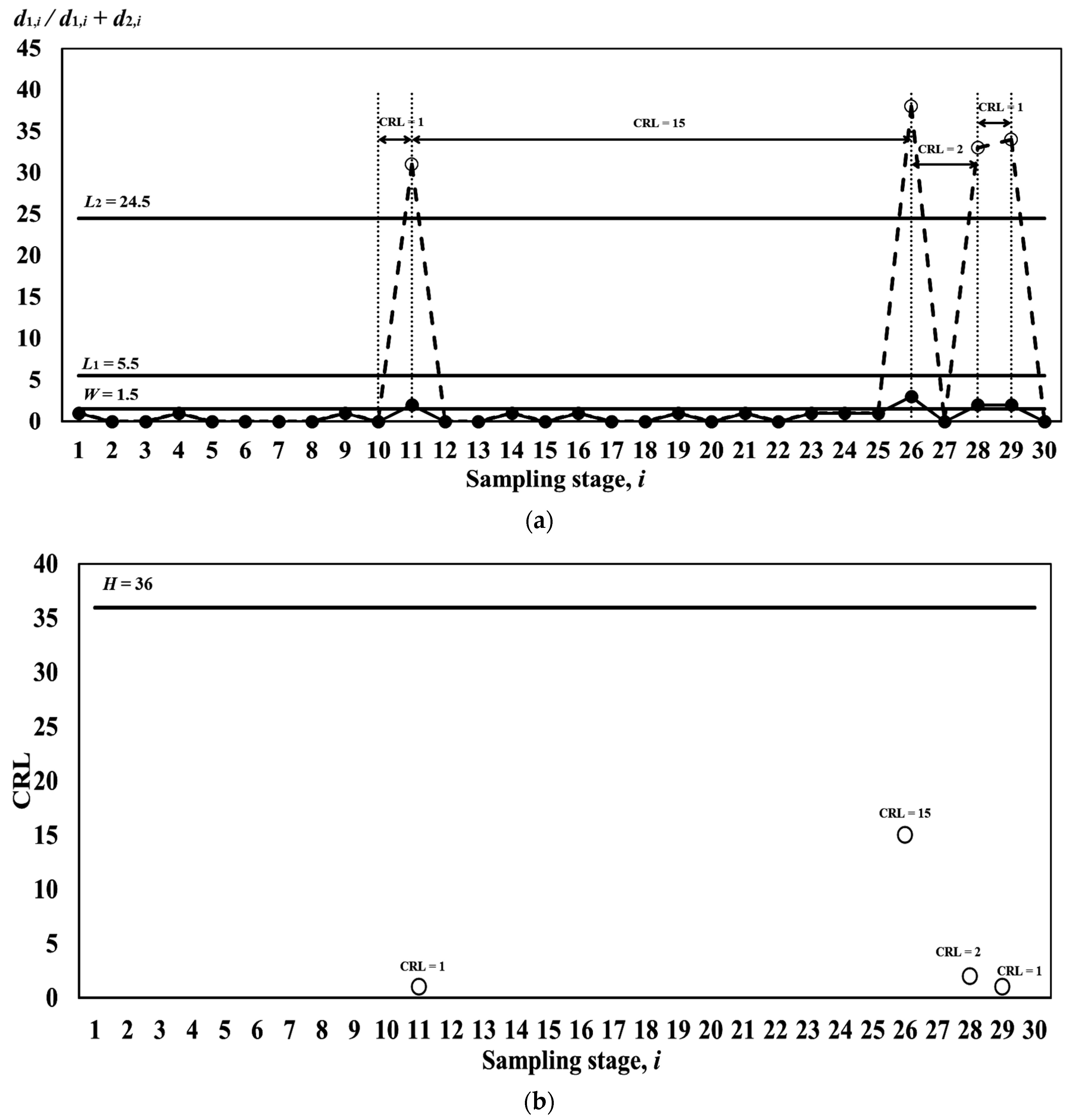
| Sampling Stage, i | First Sample (n1 = 25) d1 | Second Sample (n2 = 846) d2 | d1 + d2 | CRL |
|---|---|---|---|---|
| 1 | 1 | |||
| 2 | 0 | |||
| 3 | 0 | |||
| 4 | 1 | |||
| 5 | 0 | |||
| 6 | 0 | |||
| 7 | 0 | |||
| 8 | 0 | |||
| 9 | 1 | |||
| 10 | 0 | |||
| 11 | 2 | 29 | 31 | 1 |
| 12 | 0 | |||
| 13 | 0 | |||
| 14 | 1 | |||
| 15 | 0 | |||
| 16 | 1 | |||
| 17 | 0 | |||
| 18 | 0 | |||
| 19 | 1 | |||
| 20 | 0 | |||
| 21 | 1 | |||
| 22 | 0 | |||
| 23 | 1 | |||
| 24 | 1 | |||
| 25 | 1 | |||
| 26 | 3 | 35 | 38 | 15 |
| 27 | 0 | |||
| 28 | 2 | 31 | 33 | 2 |
| 29 | 2 | 32 | 34 | 1 |
| 30 | 0 |
Disclaimer/Publisher’s Note: The statements, opinions and data contained in all publications are solely those of the individual author(s) and contributor(s) and not of MDPI and/or the editor(s). MDPI and/or the editor(s) disclaim responsibility for any injury to people or property resulting from any ideas, methods, instructions or products referred to in the content. |
© 2023 by the authors. Licensee MDPI, Basel, Switzerland. This article is an open access article distributed under the terms and conditions of the Creative Commons Attribution (CC BY) license (https://creativecommons.org/licenses/by/4.0/).
Share and Cite
Tuh, M.H.; Kon, C.M.L.; Chua, H.S.; Lau, M.F.; Chang, Y.H.R. Evaluating the Performance of Synthetic Double Sampling np Chart Based on Expected Median Run Length. Mathematics 2023, 11, 595. https://doi.org/10.3390/math11030595
Tuh MH, Kon CML, Chua HS, Lau MF, Chang YHR. Evaluating the Performance of Synthetic Double Sampling np Chart Based on Expected Median Run Length. Mathematics. 2023; 11(3):595. https://doi.org/10.3390/math11030595
Chicago/Turabian StyleTuh, Moi Hua, Cynthia Mui Lian Kon, Hong Siang Chua, Man Fai Lau, and Yee Hui Robin Chang. 2023. "Evaluating the Performance of Synthetic Double Sampling np Chart Based on Expected Median Run Length" Mathematics 11, no. 3: 595. https://doi.org/10.3390/math11030595