Article

A Multi Parameter Forecasting for Stock Time Series Data Using LSTM and Deep Learning Model

1
Department of Computer Science, Capital University of Science & Technology, Islamabad 44000, Pakistan
2
Department of Software Engineering, Capital University of Science & Technology, Islamabad 44000, Pakistan
3
School of Digital Science, Universiti Brunei Darussalam, Jalan Tungku Link, Gadong BE1410, Brunei
4
Department of Information Technology, College of Computer and Information Sciences, Princess Nourah bint Abdulrahman University, P.O. Box 84428, Riyadh 11671, Saudi Arabia
5
Department of Information Technology, College of Computers and Information Technology, Taif University, P.O. Box 11099, Taif 21944, Saudi Arabia
6
Department of Information and Communication Technology, University of Agder (UiA), N-4898 Grimstad, Norway
*
Authors to whom correspondence should be addressed.
Mathematics 2023, 11(3), 590; https://doi.org/10.3390/math11030590
Submission received: 15 October 2022 / Revised: 12 January 2023 / Accepted: 17 January 2023 / Published: 22 January 2023
(This article belongs to the Special Issue Complex Network Analysis of Nonlinear Time Series)

Abstract

:
Financial data are a type of historical time series data that provide a large amount of information that is frequently employed in data analysis tasks. The question of how to forecast stock prices continues to be a topic of interest for both investors and financial professionals. Stock price forecasting is quite challenging because of the significant noise, non-linearity, and volatility of time series data on stock prices. The previous studies focus on a single stock parameter such as close price. A hybrid deep-learning, forecasting model is proposed. The model takes the input stock data and forecasts two stock parameters close price and high price for the next day. The experiments are conducted on the Shanghai Composite Index (000001), and the comparisons have been performed by existing methods. These existing methods are CNN, RNN, LSTM, CNN-RNN, and CNN-LSTM. The generated result shows that CNN performs worst, LSTM outperforms CNN-LSTM, CNN-RNN outperforms CNN-LSTM, CNN-RNN outperforms LSTM, and the suggested single Layer RNN model beats all other models. The proposed single Layer RNN model improves by 2.2%, 0.4%, 0.3%, 0.2%, and 0.1%. The experimental results validate the effectiveness of the proposed model, which will assist investors in increasing their profits by making good decisions.
MSC:
68Rxx; 68-XX; 68Uxx; 68T07

1. Introduction

One of the most significant issues in the financial world has always been the tendency of stock price fluctuation. Many internal and external factors, such as the local and global economic climate, current affairs, industry prospects, financial information from publicly traded firms, and stock market activity, have an impact on stock prices. The traditional analysis method is used to examine the stock market’s behaviour. Traditional analysis is based on two methods: fundamental analysis and technical analysis. External factors such as interest rates, exchange rates, inflationary trends, industrial policies, interactions with other nations, economics, and political considerations are heavily weighted in the basic examination method. The technical examination approach, on the other hand, concentrates on stock prices and trade volume [1]. The stock market is widely recognized for being a highly volatile system. Many studies have been conducted on forecasting stock prices, and many techniques have been used for this [2]. Based on technical analysis, researchers used time series data to forecast the short-term stock price using long-term data, and such methodologies were based on models such as LSTM, GRU, meta learner [3], CNN-LSTM, LSTM [1,4], LSTM [5], CNN [6], and CNN-SVM [7].
Many researchers have proposed various deep-learning methods to improve stock price forecasting, such as the close price for the next day, week, month, or year. However, a question still arises. What effect do deep learning models have on short-term predictions? To answer that question, deep learning models can recognize the non-linear and complex patterns to analyze the complex patterns of financial stock data. Deep learning models help in recognizing the patterns and help us forecast for the next day, weeks, and months. A second question arises. What effects does multi-parameter stock price modeling have on short-term predictions? A third question arises. Why do the stock prices not forecast more than one parameter? To answer this, a new methodology is present to forecast the two stock parameters, the close price and the high price. The methodology is based on three models: CNN, LSTM, and RNN. These three models all receive data simultaneously, process it in parallel, and then produce results. To forecast the two stock parameters, close price and high price, for the next day, the best model with the lowest error rate will be chosen using the selection method. The daily transaction data of the Shanghai Composite Index (000001) is taken as a data set from 3 July 1997, to 24 January 2022, in which the training set contains 4761 trading days data, and the validation and testing set contains 1190 trading days data.
This study makes a contribution as described below.
  • A new methodology is proposed to forecast two stock parameters, close price, and high price, by analyzing time series data on stock prices.
  • Comparing the hybird deep learning forecasting model with other stock price forecasting methods, the proposed method demonstrates that it is the most precise and suitable method for the forecasting of stock prices.
The high price is forecasted primarily due to the high fluctuation of stock prices in the stock market and the stakeholders’ demands. The stock’s high price is significant because it serves as a barometer of where the stock’s price has been trading, giving traders and investors information about the stock, possible points of entrance and exit, and a look into the stock’s possible future trading range. A high price data point on a stock chart represents the stock’s highest value during a trading day. For traders and investors, a high price offers useful information that helps make various trading decisions.
This paper is divided into the sections listed below. The associated work is covered in Section 2. Section 3 provides an explanation of the proposed methodology. The experiment in Section 4 is followed by a discussion of the findings. Things come to a conclusion in Section 5.

2. Related Work

We review the research on previously proposed stock price forecasting methods, and the analysis table is shown in Table 1. The core of these approaches was a combination of deep learning and machine learning techniques. Srilakshmi. K et al. [4] used Bi-LSTM, CNN-LSTM, three layer LSTM, single layer LSTM, and three layer LSTM were all employed to anticipate the close price of TCS stock for the following day. In comparison, CNN-LSTM and Bi-LSTM performed outstandingly as compared to the single layer LSTM and three layers LSTM. Lu et al. [1] used the CNN-LSTM technique to forecast the close price for the next day of the Shanghai Index (000001). The basic purpose of CNN was to retrieve the best features from the data, and the close stock price was predicted using the LSTM algorithm. The problem identified was that the CNN could not retrieve the best feature from the input data. Mehtab et al. [6] forecasted the close price of the NSE NIFTY 50 index using the deep learning CNN model. Using univariate and multivariate methodologies, three CNN models with different input data sizes and network configurations were built, significantly enhancing the forecasting framework. Yadav et al. [8] used the deep learning LSTM base technique to forecast the close price of the NSE NIFTY50 index. Stateful and stateless LSTMs were compared, and it was determined that stateless LSTMs were more stable than stateful LSTMs. Based on the results, a stateless LSTM model was found to be superior for time series forecasting challenges due to its higher stability. Sheng Lu et al. [9] forecasted the close price of the Taiwan Stock Exchange (TWSE) using the deep learning LSTM model. The main purpose was to replace the RNN model with the LSTM model due to the long-term memory because RNN was unable to maintain the long-term data.
Chen et al. [10] used CNN, BiLSTM, and an attention mechanism-based model to forecast the closing prices of various firms, including China Unicom, the Shanghai Composite Index, and the CSI 300. The features were retrieved from the input data using CNN. Efficient channel attention was combined with BiLSTM to improve the network’s sensitivity to forecast the stock price. Samarawickrama and Fernando [11] forecasted the closing price of the Colombo Stock Exchange (CSE) using deep learning models, and the four deep learning models were FFNN, SRNN, LSTM and GRU. After analyzing the generated results, the forecasting accuracy of the feed forward neural network was approximately 99%. When compared to the feed forward network, SRNN and LSTM produced lower error rates; however, on some occasions, SRNN and LSTM produced high error rates. When compared to other models, GRU produced a high error rate. Ojo et al. [2] forecasted the close price of the American Stock Exchange NASDAQ Composite (IXIC) using stacked LSTM, a deep learning technique. The results showed that the accuracy had improved while forecasting the stock price. Li et al. [12] forecasted the close price of two different data sets JQData and Pingan Bank—using a hybrid deep learning approach. The main purpose of CNN was to retrieve the best features from the input data. The LSTM model takes the output of the CNN model as an input and performs calculations to predict stock price and the attention mechanism used on the LSTM model to improve the scalability of the CNN-LSTM model. The experiment result of the CNN-LSTM model was analyzed with SVM, LSTM, and GRU results. Based on the results, the CNN-LSTM model outperformed the other models.
Lounnapha et al. [13] forecasted the close price and trend of three Thai stock exchange companies using the CNN model. The sliding window was used, and its size was the same as the input size. There was no overlap between the two consecutive windows when the sliding window moved right on each iteration. The results demonstrated that the CNN model performed admirably on the current day. Fabbri and Moro [14] used the LSTM model to forecast the close price of the trading Dow Jones for the next day. The LSTM model result was analyzed with the FFNN results. The generated results show that LSTM performed better than feed forward neural network. Prachyachuwong et al. [15] used LSTM and BERT to forecast the stock trend of the Thailand Futures Exchange SET50 index based on the close price. LSTM was used for the numerical data and BERT for the textual data. Kesavan M. et al. [16] proposed a methodology based on NLP and LSTM models to forecast stock prices. NLP was used to analyze the textual data (financial news), whether the financial news was positive or negative, and LSTM was used to forecast the historical financial data. Batool el al. [17] examined the sharing economy (SE) of selected countries in COVID-19 lockdown using a difference-in-difference estimation technique and Google trends data. The analyzed results verified that online services gain profit such as e-commerce, online streaming services, etc, while, on the other side, transport company series and accommodation sectors have gone into loss, and many people have become unemployed.
By studying the literature, we see that the researchers have forecasted the single stock parameter, such as the close price. Most researchers use the LSTM model for forecasting and the CNN model for retrieving the best features from the input data.
Table 1. Analysis of previous studies.
ReferenceAuthors/Published DateTechnique/DatasetRemarks
[4]Srilakshmi.K, Sai Sruthi.Ch Published in 2021Using Single Layer LSTM, Three Layer LSTM, CNN-LSTM, ConvLSTM, BiLSTM to forecast historical stock data using TCS stock as data setTo forecast the close price, ConvLSTM and BiLSTM were performing better than other models. CNN-LSTM, single layer LSTM, and three layer LSTM still improved when the epoch was increased.
[15]Prachyachuwong, Vateekul Published in 2021Using LSTM for historical stock data and BERT for textual data on using SET50index as data setTo forecast the stock close price. he suggested model outperformed the base paper in terms of performance. The generated results verified that proposed model had improve with an accuracy of 61.28% and F1 of 51.58% and achieved highest annualized return of 8.47%
[1]Lu et al. Published in 2020Using CNN for features extraction and LSTM for the forecasting historical stock data using Shanghai Composite Index (000001) as data setTo forecast the stock close price, CNN-LSTM was used. The generated results verified that they were performing better than other models. The limitation in this paper was that of the model architecture design. The problem was that the CNN was unable to retrieve the best features from the input data.
[6]Mehtab, Sen Published in 2020Using CNN forecasting historical stock data using NIFITY 50 index as a data setStock close price was forecasted using CNN. The results verified that CNN was performing better than machine learning models and able to extract more features than machine learning models. CNN gave more accurate accuracy in multivariate analysis as compared to univariate analysis.
[6]Sidra Mehtab, Jaydip Sen Published in 2020Using CNN for forecasting historical stock data using NIFITY 50 index as a data setTo forecast the stock close price, CNN was used. The results verified that CNN was performing better than machine learning models and able to extract more features than machine Learning models. CNN gave accurate accuracy in multivariate analysis as compared to univariate analysis.
[8]Yadav et al. Published in 2019Using LSTM for forecasting historical stock data using TCS stock as a datasetTo forecast the stock adj-close price, LSTM was used. The results verfied that stateless LSTM performed better as compared to stateful LSTM
[9]Lin et al. Published in 2018Using LSTM for forecasting historical stock data using TWSE stock as a datasetTo forecast the stock close price, LSTM was used. LSTM resolved the problem of storing long-term data, which was faced in RNN model.

3. Proposed Methodology

To perform the forecasting of two stock parameters, the close price and the high price were used. Three models—CNN, LSTM, and RNN—will be used. These three models obtain the input and start processing in parallel and generate output. The selection method will select the best model on the of the error rate bases. Figure 1 displays the architecture diagram for proposed model.

3.1. CNN

Lecun et al. [18] proposed the CNN network concept in 1998. CNN performs well in both natural language processing and image processing (NLP). It can be used to forecast time series with success [19]. We can train a CNN model to improve forecasting and accuracy using multivariate time series data, and we are going to investigate the forecasting power of CNN in this work.
A CNN is made up of three primary layers a convolution layer, a pooling layer, and a fully connected layer, as shown in Figure 2. The convolution layer makes an effort to retrieve the best features from the 1-D matrix and perform calculation to provide a convoluted output, as shown in Equation (1).
C L t = t a n h ( x t w t + b t )
where C L t is the convolution output, activation function is tanh, x t is input value, w t is the weight, and b t is the bias.
The pooling layer takes the output of the convolutions as an input. The max pooling function is used to choose the heavily weighted features in the pooling layer. The pooling layer’s output is passed to the flatten layer. The flatten layer’s primary function is to convert the data into a single array form. The fully connected layer receives the flatten layer’s output and processes it to obtain the results.

3.2. LSTM Model

Schmidhuber et al. [21] suggested the LSTM network model in 1997. In the training processing, long-term memory issue and the vanishing gradient problem affect the RNN models frequently. A network model called LSTM was created to handle the long-term memory issues with vanishing gradient problems in RNN [1,8,9,10]. The model uses a gate control mechanism to control the information flow and carefully chooses how much incoming data should be stored for each time step. The core LSTM unit consists of three control gates an input gate, an output gate, and a forgetting gate, which is seen in Figure 3.
The forget gate is used to store important information in the cell state while removing unnecessary information. It takes two values as input, the current input value and the most recent output value of the previous state, and uses the sigmoid function to do computations to get the forget gate result value, which is a number between 0 and 1, as shown in Equation (2).
F G t = σ ( ( W f g h t 1 ) + ( W f g x t ) + b f g )
The input at that time step is x t , and the recent last state value is denoted by h t 1 . The weight is denoted by W f g , and bais is denoted as b f g . The forget gate activation function output is represented by F G t . The previous cell state is then multiplied by the forget gate activation function output to decide whether or not the prior data should be stored in the cell, as shown in Equation (5).
The input gate is used to provide fresh data to the cell state. It requires the current input, as well as the most recent state value, as inputs. The calculation is performed on the input values, and the sigmoid function is used as a filter to obtain output between 0 and 1, as shown in Equation (3).
I G t = σ ( ( W i g h t 1 ) + ( W i g x t ) + b i g )
where W i g is the weight, h t 1 is the recent last state value, x t is the input at that time step, b i g is the bias, and I G t is the input gate result.
A new cell function is created to obtain all possible values in the cell state. This function also takes two inputs—the current input value and the recent last state value. The calculation is performed on the input values, and tanh activation action is applied as a filter to obtain output between −1 to 1, as shown in Equation (4).
C t ˜ = t a n h ( ( W i g h t 1 ) + ( W i g x t ) + b i g )
where W i g is the weight, h t 1 is the recent last state value, x t is the input at that time step, b i g is the bias, and C t ˜ is the cell state function value at that time step.
The result of the cell function and input gate output is multiplied and added to the cell state as shown in Equation (5).
C t = C t 1 F G t + I G t + C t ˜
The basic purpose of the output gate is to give the best feature as an output. The output gate performs the calculation using two inputs the current input value and the most recent state value at that moment. The value between 0 and 1 is filtered using the sigmoid activation function to get the output value, as shown in Equation (6)
O t = σ ( ( ( W o g h t 1 ) + ( W o g x t ) ) + b o g )
where W o g is the weight, h t 1 is the recent last state value, b o g is the bias, and O t is the output value at that time step
In order to filter values between −1 and 1, a new cell state function is developed that applies the tanh activation function on the cell state, as shown in Equation (7).
O C t ˜ = t a n h ( C t )
where C t is denoted as the cell state and O C t ˜ is the function cell state’s output value.
The cell state function value is multiplied by the output value, and the result is transmitted to the following hidden layer, as shown in Equation (8).
O o g = O t O C t ˜

3.3. RNN Model

RNN is capable of capturing the time series data. RNN contains hidden layers to calculate a large number of the input sequence, in contrast to the traditional ANN, which is unable to memorize the previous historical information of the sequences. Recurrent neural networks are composed of multiple layers, and each layer contains multiple nodes. A, B, and C are the network’s parameters. This is seen in Figure 4.
The input, hidden, and output layers are denoted by the letters X, H, and Y, respectively. To enhance the output of the model, the network parameters A, B, and C are used. Input at x t and x t 1 at any given time t are combined to form the current input. To make the network better, output is always being gathered from it, as shown in Equation (9).
h t = f ( h t 1 , x t )
The input data x are passed to the model via input layer A, illustrated in Figure 4, and the central layer h contains multiple hidden layers, each with its own activation functions, weights, and biases. tanh is the activation function. The previous concealed state is represented by h t 1 , and its weight is represented by W p h . The weight of the current hidden state is W x h , while the current input is x t , as shown in Equation (10).
h t = t a n h ( W p h h t 1 + W x h x t )
The output layer ‘y’ receives the hidden layer’s output as an input. Some calculations are performed to obtain the real outcome, as illustrated in Equation (11). The actual result is the forecasted value. W h y is the weight of output, h t is weight of hidden layer, and y t is the output at time t, as shown in Equation (11).
y t = W h y h t
A RNN receives its two inputs from the recent past and the present. This is vital because the data sequence contains necessary details about what will occur next, which allows a RNN to carry out tasks that other algorithms are unable to do.
In the literature, various approaches were used for the prediction such as, neural network-based intelligent decision-making [24], deep learning models [25,26,27,28], machine learning-based methods [29,30,31,32], and CNN, RNN and LSTM based methods [33,34,35].

3.4. Selection Method

After receiving the findings of the error rates of these three models, CNN, LSTM, and RNN, the selection method will select the optimal model with the highest accuracy. The selection approach is effective based on the R 2 evaluation matrix. The model with a result which is closer to or equal to 1 is selected by the selection method.

4. Experiment

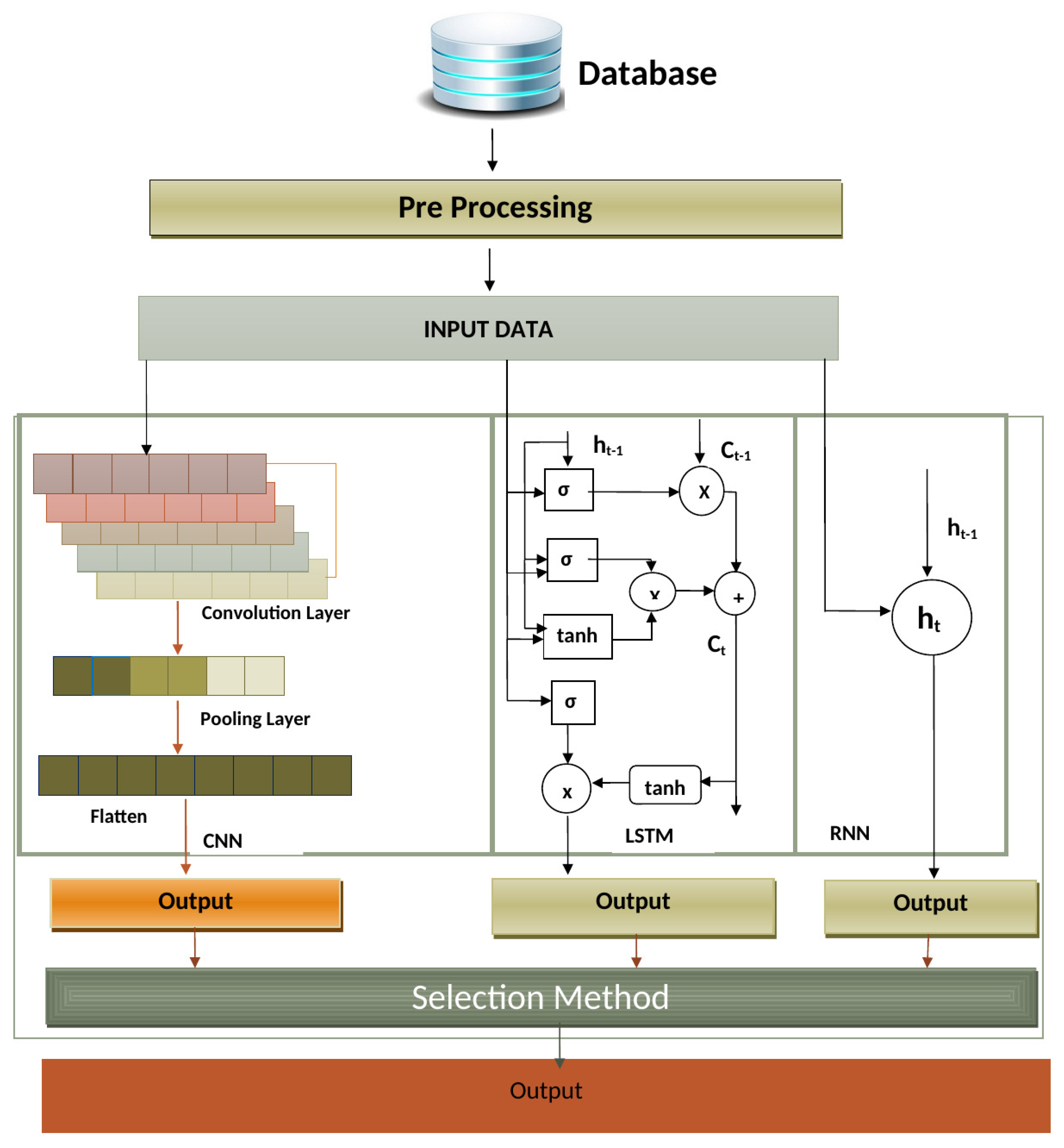
To evaluate the proposed model’s efficacy, it is compared to CNN, RNN, LSTM, CNN-RNN, and CNN-LSTM models. On the same data set, the models are trained and tested. The open price, high price, low price, close price, adj-close price, and volume are the stock parameters that influence it.

4.1. Tools and Technology

  • Python: It is a smart, adaptable, and versatile programming language. Being clear and easy to read, it makes a fantastic first language. It is the core programming language for Web development, machine learning, and data science.
  • Microsoft Excel: The spreadsheet application Microsoft Excel was developed by Microsoft. Tools for calculating and computing, charting, and pivot tables are all included. As a database, Excel is used. The data are retrieved and executed using Excel. The graphs of the outputs are also created using Excel.
  • Google Colab: It is an online tool that facilitates the developer to implement the code in the standard environment without relying on the local computer resources and provided opportunities to the developers to work in any environment.
  • Keras: It is a python API that helps the developer to speed up the implementation of the experiment using simple methods and libraries and remove a huge coding load from a developer.
  • Pandas: It is a Python toolkit that is free and open-source for tasks including data science, analysis, and machine learning. It is built for the multi-dimensional array-supporting library Numpy. These tasks include data cleaning, data filling, data normalisation, data visualisation, data loading and storage, statistical analysis, and much more. It is used for reading data, assessing it, altering it, and then saving it. Using the Pandas library, all of these things are possible.
  • Numpy: It is an open-source python library. Python has lists that function similar to arrays. Arrays are mostly used in data studies.

4.2. Data Set

The data for this experiment is taken from the Shanghai Composite Index (000001). From 3 July 1997 to 24 January 2022, daily trading data for 5951 trading days were collected using the Yahoo Finance database. Data contain the open price, high price, low price, close price, and volume, as shown in Table 2. The data for the training set are 4751 days long, while the testing data set is 1190 days long.

4.3. Implementation of Model

First, the data taken from the database are pre-processed to remove the null values in the data set. After pre-processing, normalization is used to transform the set of data to be on a similar scale. To normalize the data, data standardization is used. In data standardization, Z-Score standardization is used, and the formula is shown in Equations (12) and (13).
Z = X μ S
X = Z S + μ
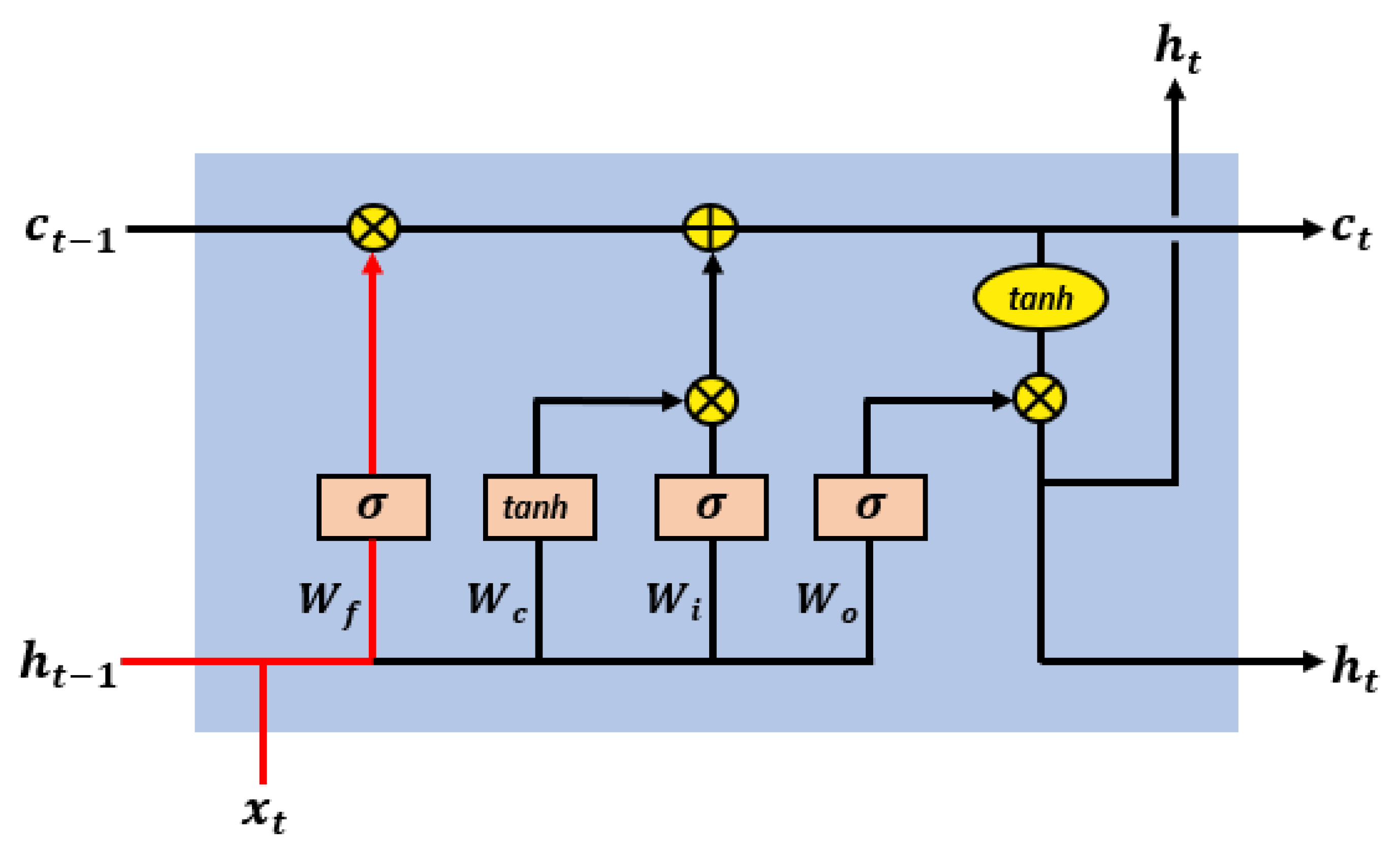
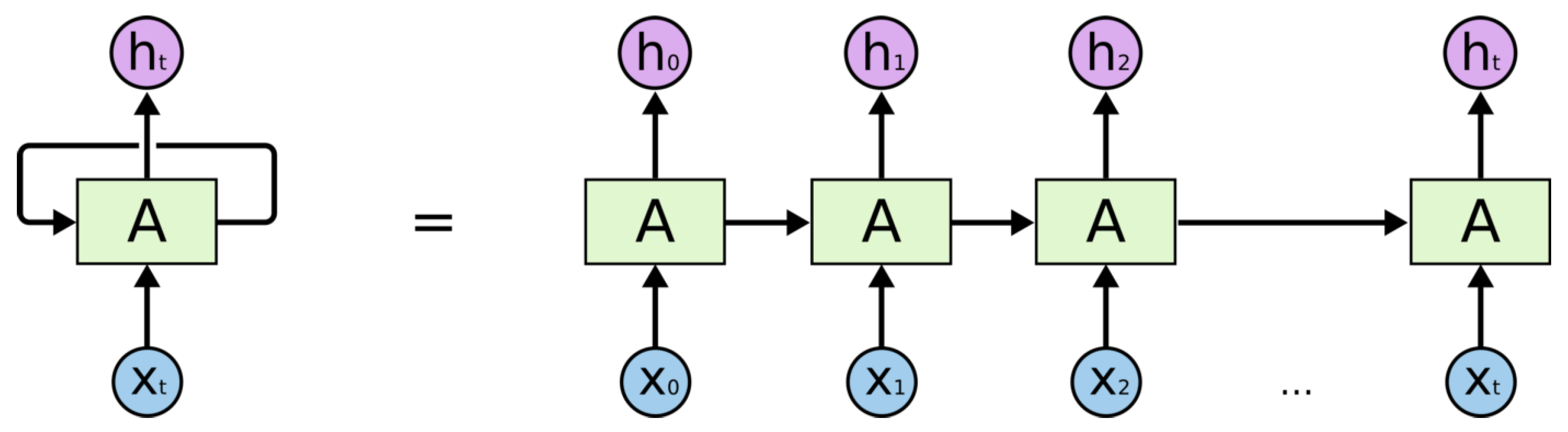
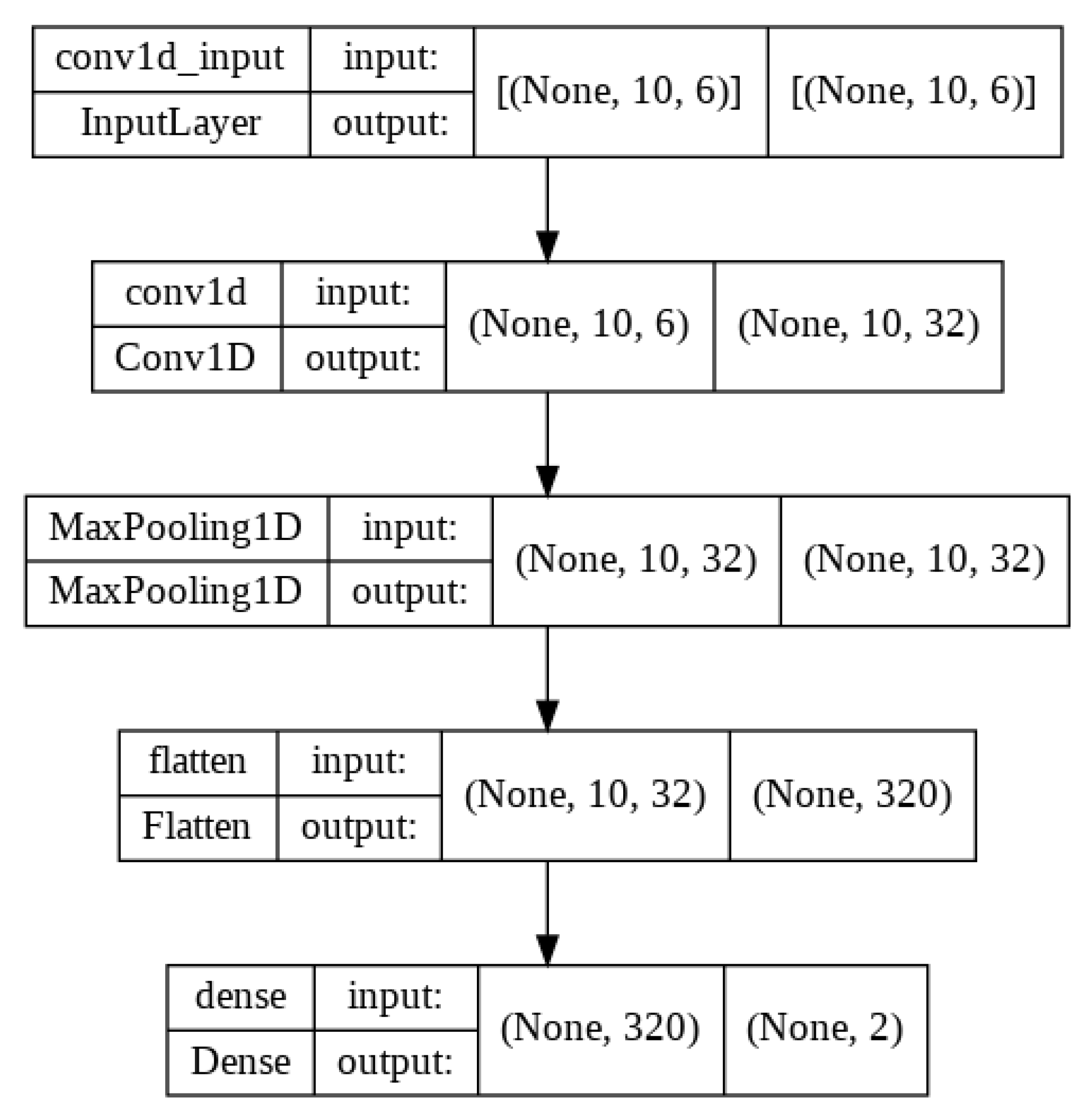
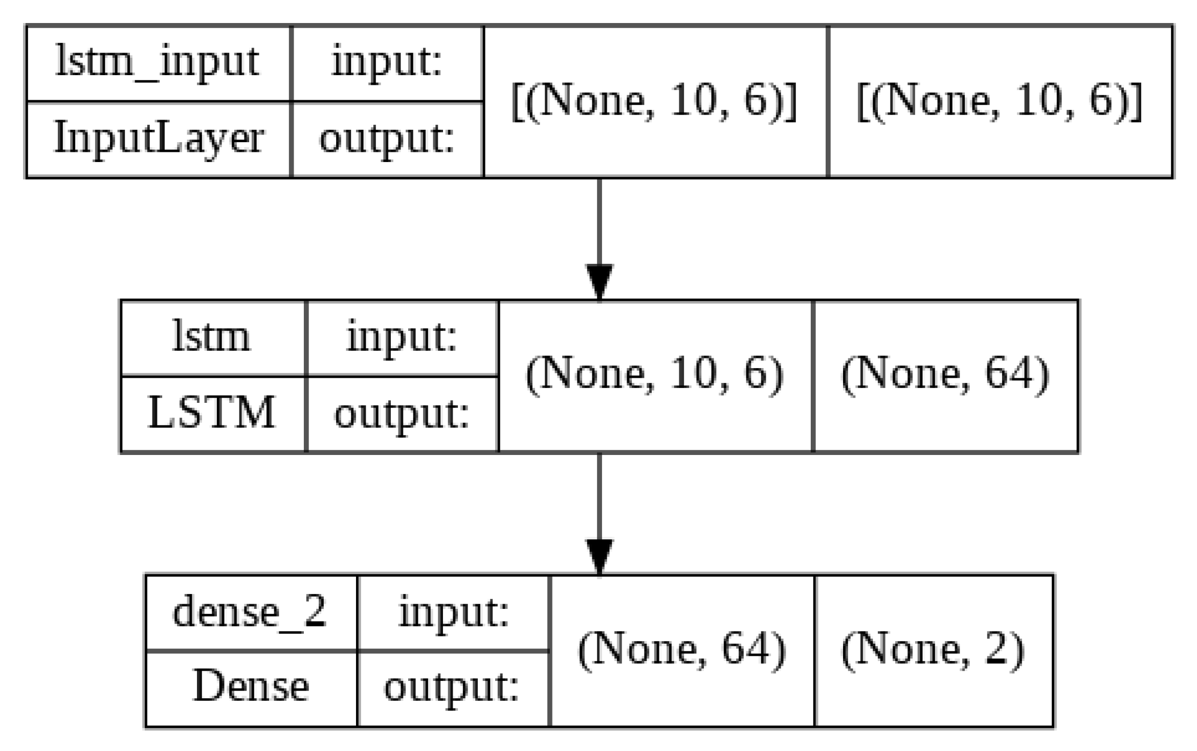
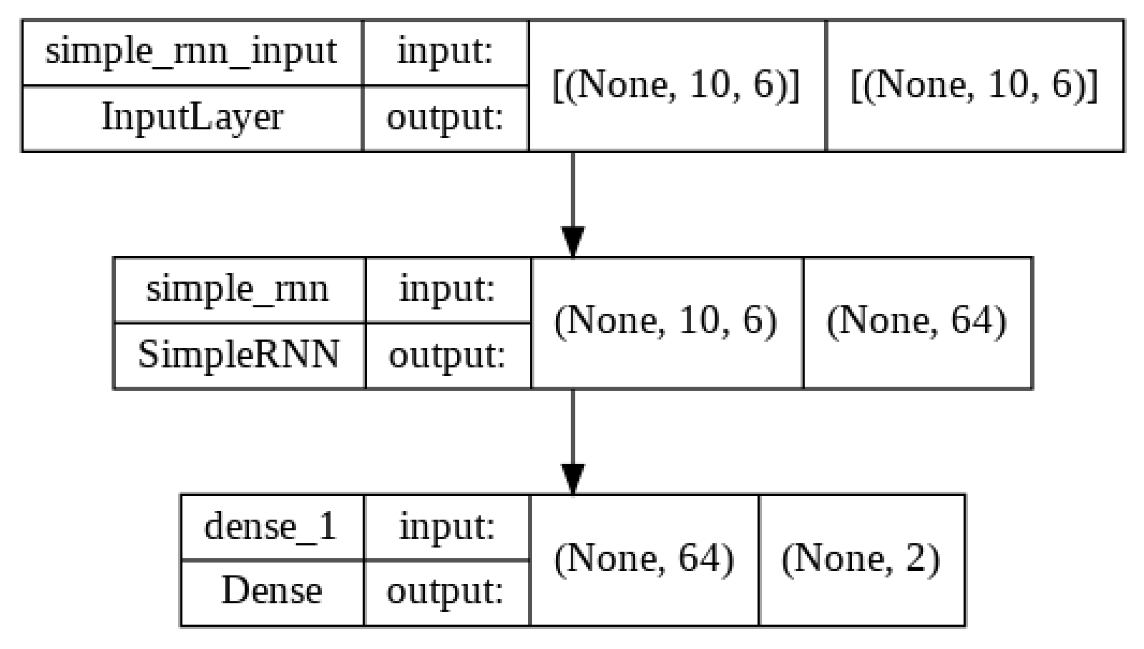
Table 3 shows the proposed methodology (CNN-LSTM-RNN model) parameter settings for this experiment. The CNN-LSTM-RNN network’s parameter values demonstrate how the particular model is constructed. The input for the 3-D vector is (None, 10, 6), where 10 is the sample size and 6 is the number of input features. As input, the data are fed into the RNN Layer, LSTM Layer, and one-dimensional convolution layer.
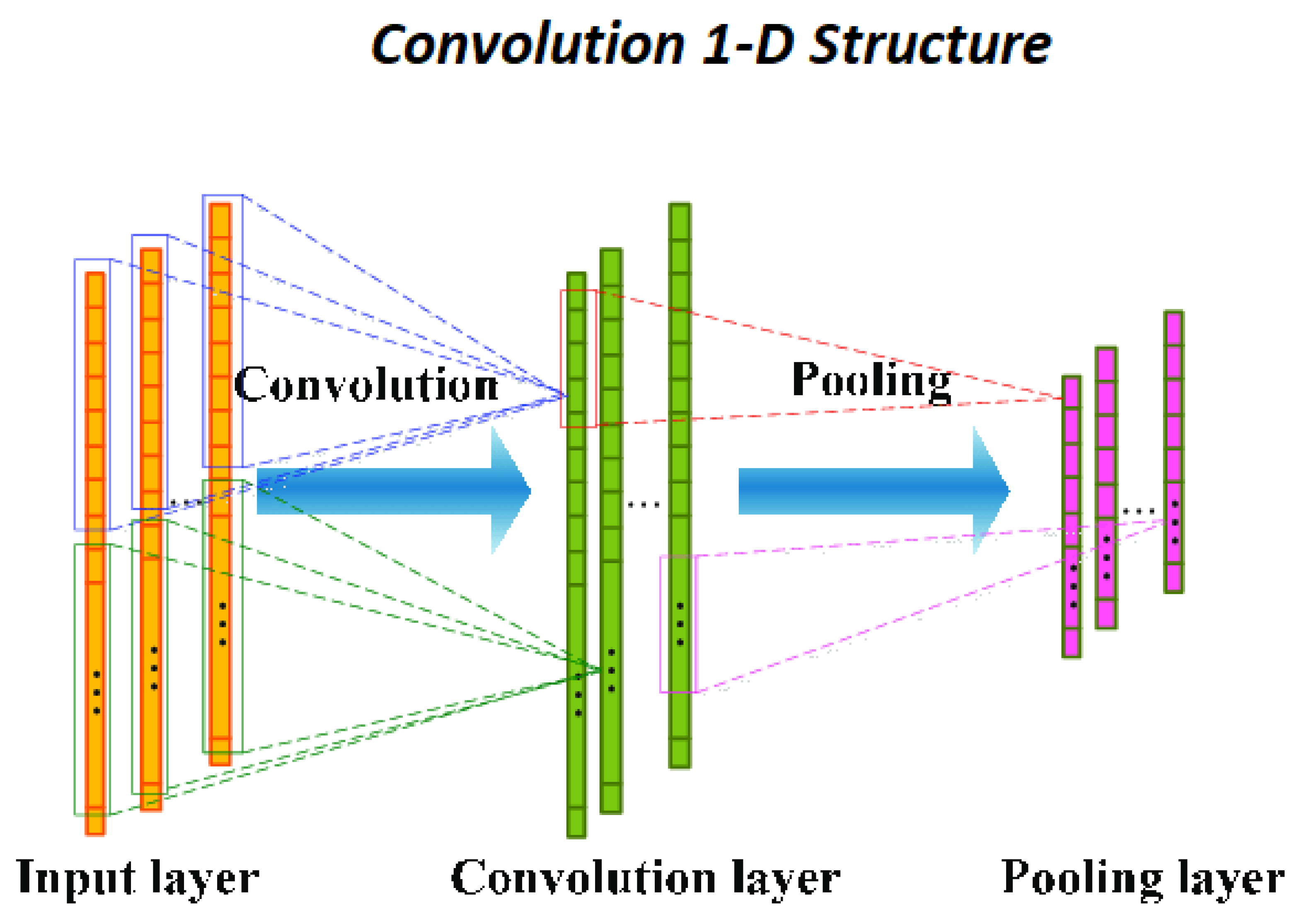
In CNN, the best feature is recovered using the convolution layer, which outputs as 3-D vector (none, 10, 32), with 32 filters, and a kernel size of 1. The pooling Layer receives the convolution output. The pooling layer uses max pooling, which moves once for each output and has a max pooling size of two and a stride of one. Flatten layer takes input of pooling layer output and converts all the output into a single dimension. The fully connected layer takes input of flatten layer output and performed calculations and displays the two forecasting stock parameters values for the next day as a result. The model structures of these three models are shown in Figure 5, Figure 6 and Figure 7.
Both the LSTM and RNN networks are running at the same time. These LSTM and RNN layers provide the input. The input data are passed from 64 units. These units carry out calculations and then provide results. The output layer then receives these outputs. In the end, the output layer does certain calculations and provides two forecasts the close price and the high price for the next day.
The selection process is used to choose the best model that performs better than the other two. The R 2 is used to make the selection. The R 2 is discussed in the following section.

4.4. Evaluation Method

MAE, RMSE, and R 2 are used for assessing the forecasting performance of the CNN-LSTM-RNN based model.
1.
MAE
MAE is used in resolving learning difficulties into optimization problems because it is most commonly utilized for the loss functions and error measure of regression problems.
M A E = i = 1 n | Y i X i | n
In this case, Y i represents the prediction, X i is the actual value, and n represents the total number of samples or records.
2.
RMSE
One of the methods most frequently used to evaluate the accuracy of forecasting models is RMSE. It shows how far the observed value varies from the actual value using Euclidean distance. The difference between forecast value and actual value for each sample are considered.
R M S E = i = 1 n ( Y i X i ¯ ) 2 n
3.
R 2
For linear regression models, R 2 is a goodness-of-fit indicator. R 2 is a metric that expresses the degree to which your model explains the dependent variable. The R 2 formula is used to calculate the amount of variance in y that can be explained by x-variables. The scale runs from 0 to 1.
R 2 = 1 S R T R
where TR is the total square sum and SR is the sum of square residuals.

4.5. Results

After performing the process to train the proposed methodology(CNN-LSTM-RNN) in which three models CNN, LSTM, and RNN are trained parallel on the training data set. After completing the training process, the validation is performed to select the best model. After getting the error rates, the selection method selects the best model on the basis of R 2 . In this case, the selection method selects the RNN model because its R 2 is closest to 1. To assess the model’s effectiveness, evaluation is done using the testing data set. A forecast is made using the test data set. After testing, the error rates of models are calculated as displayed in Table 4.
The model’s validation findings are examined. The validation results verified that the RNN model is trained better than other models because its validation results are greater than the CNN and LSTM models and closest to 1. Evaluation of model performance is performed on the test data and calculated on basis of the MAE, RMSE, and R 2 , and we see that the RNN model has less MAE and RMSE while, on the other hand, R 2 is closest to 1, which means that RNN gives accurate results.
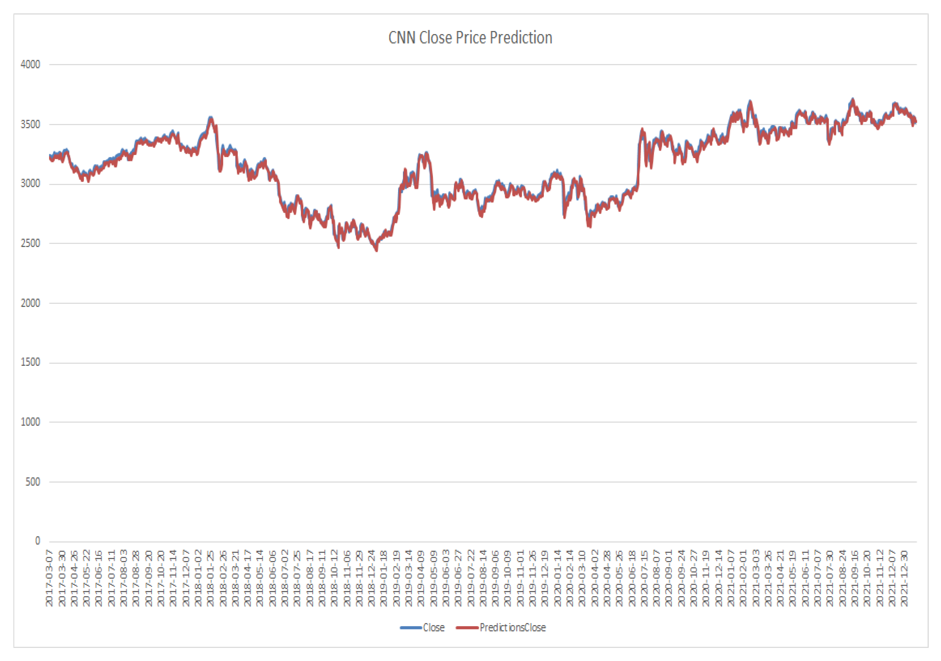
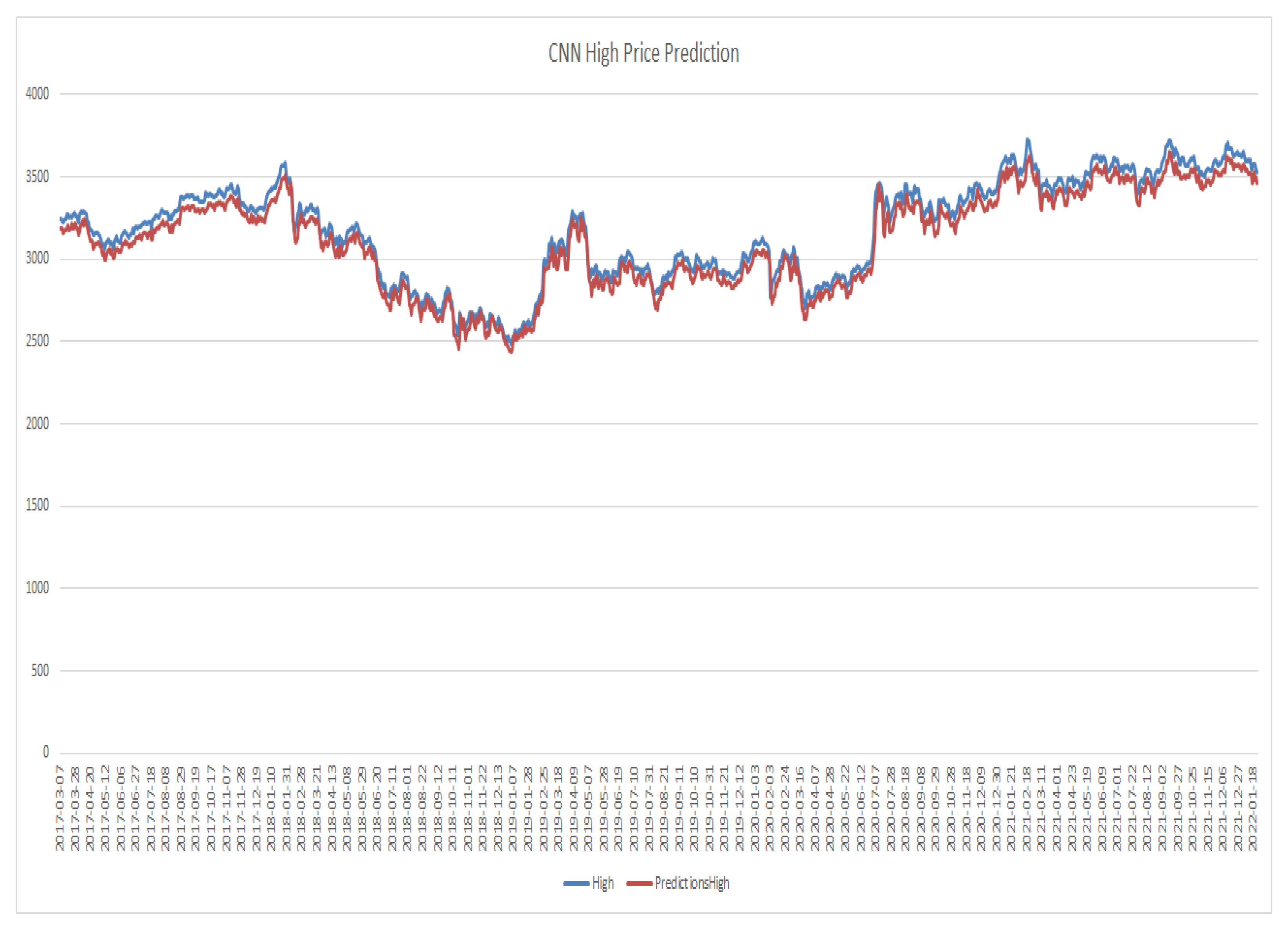
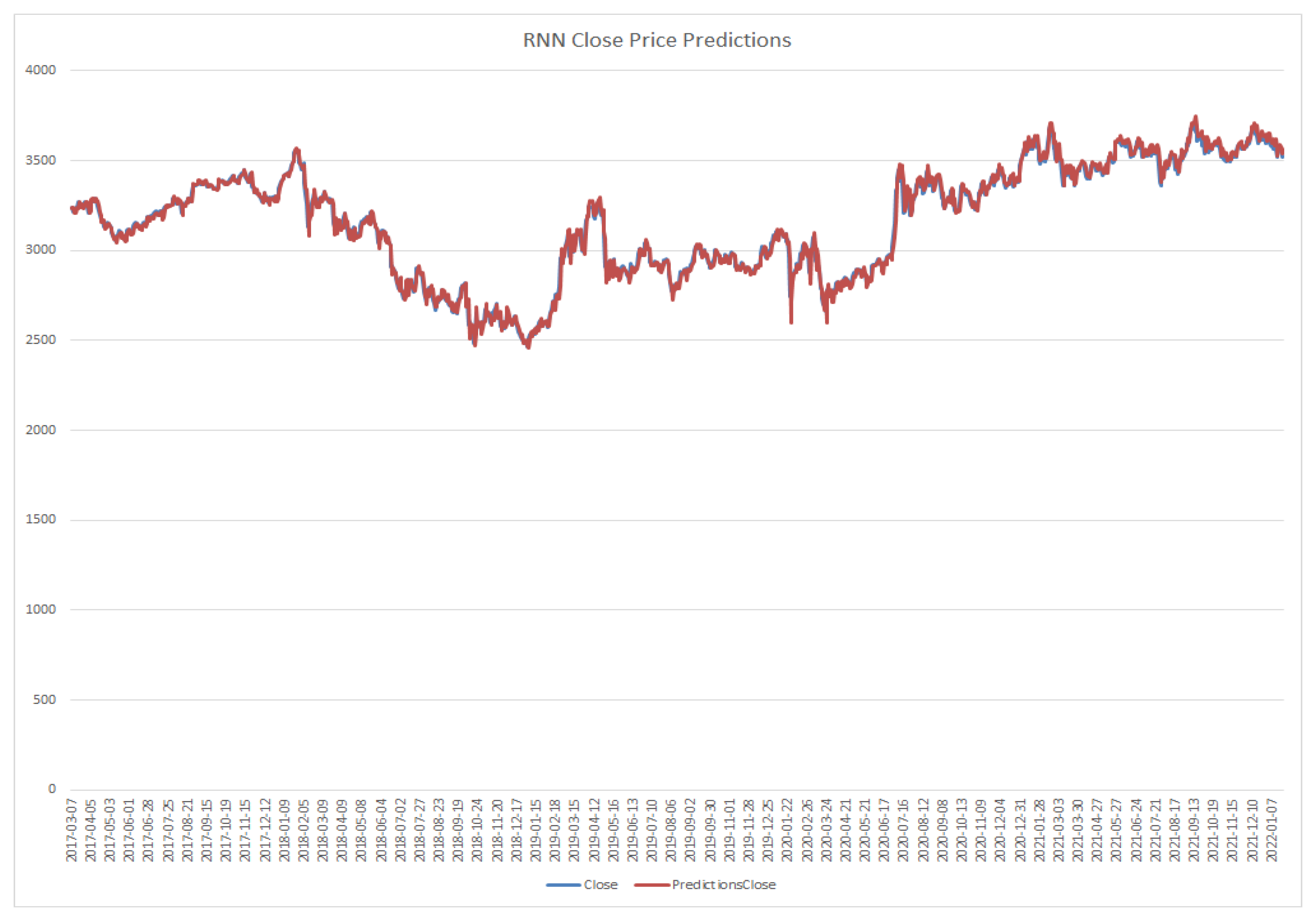
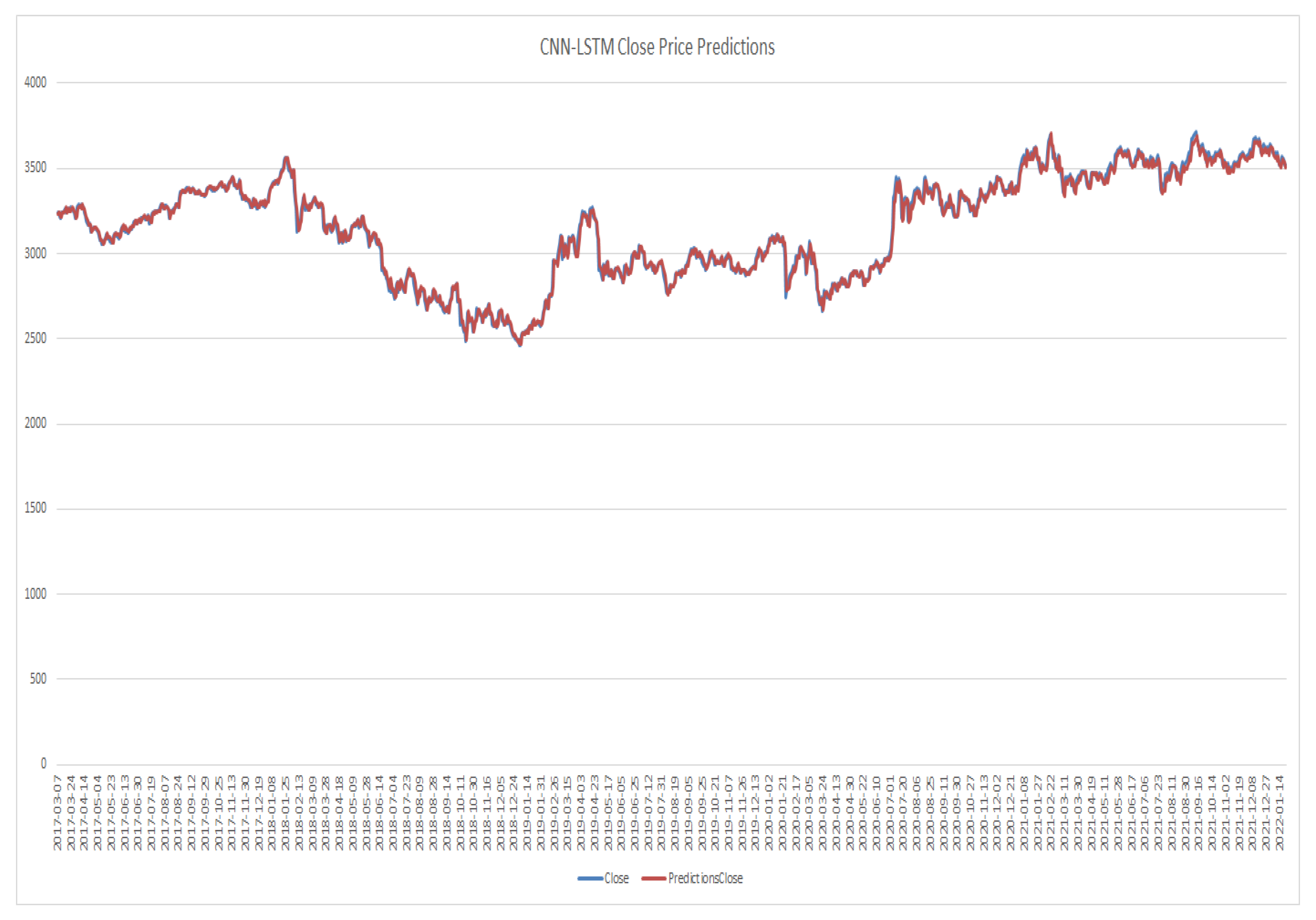
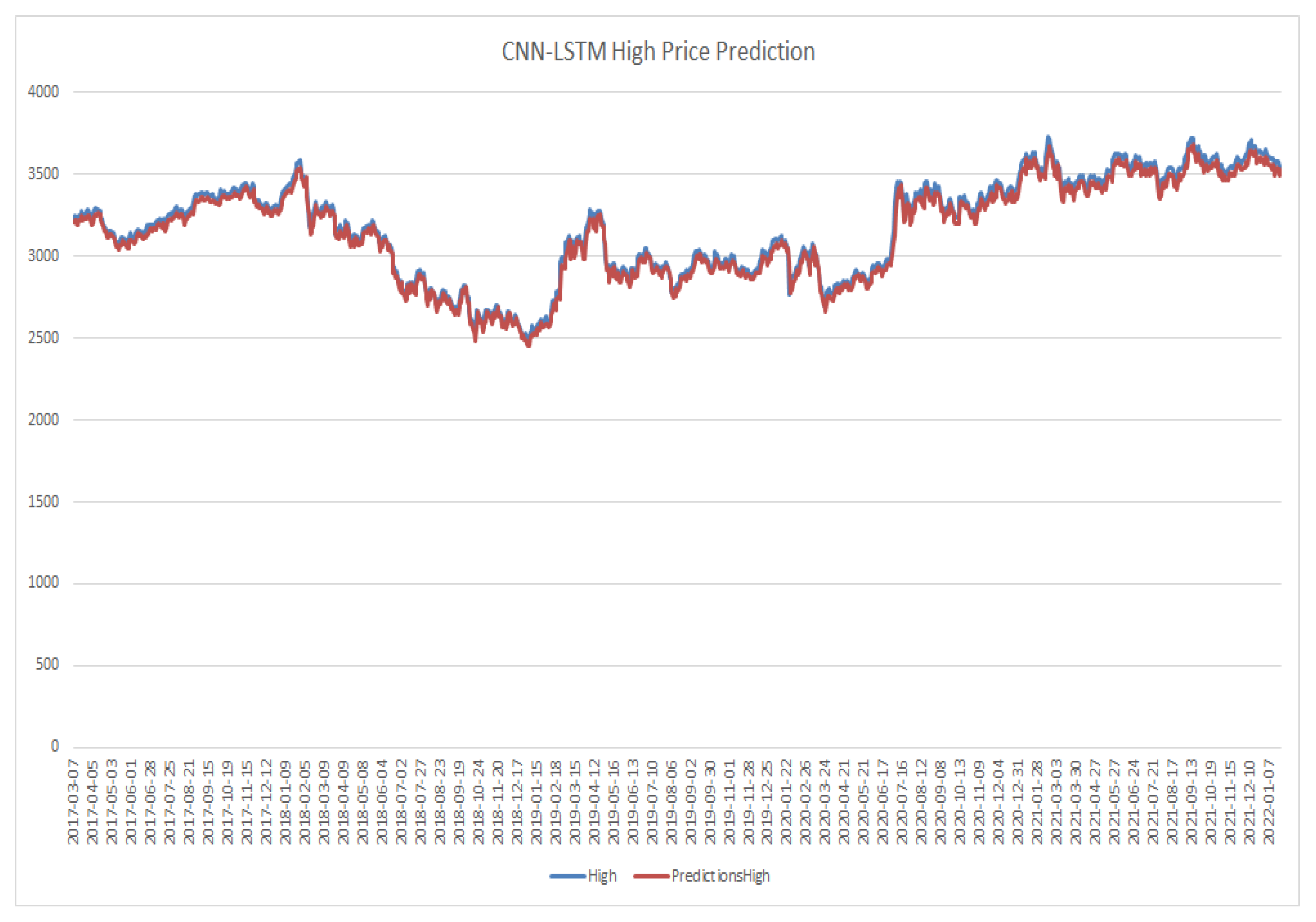
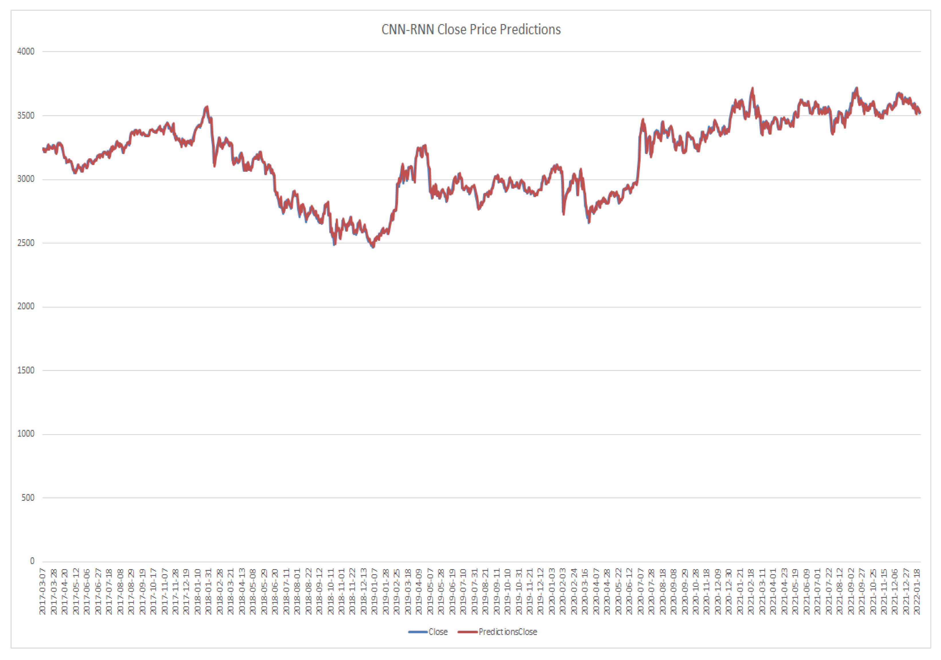
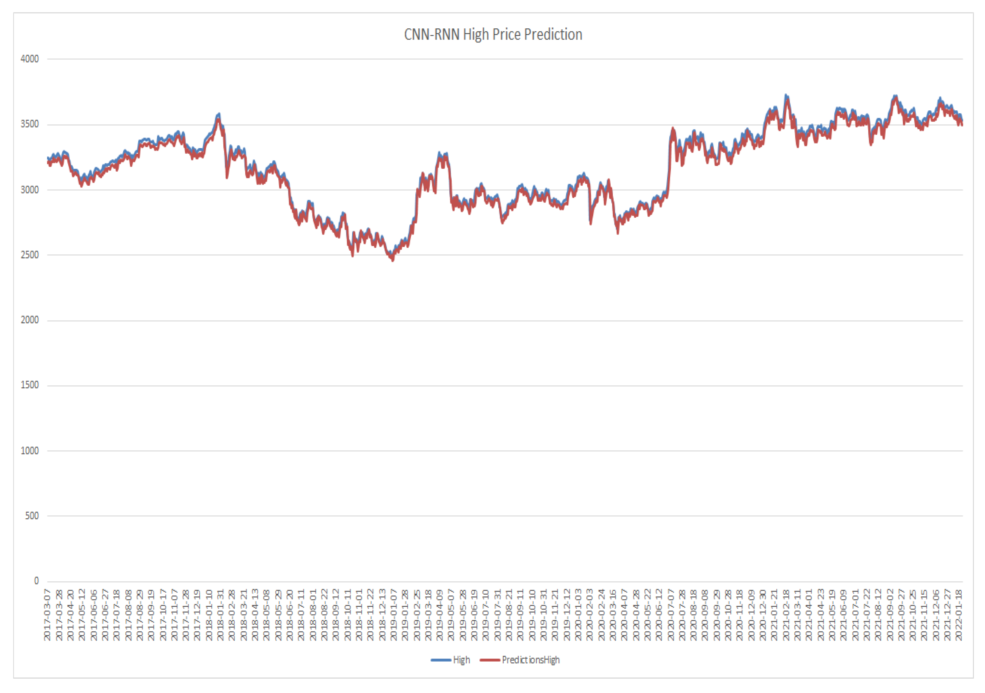
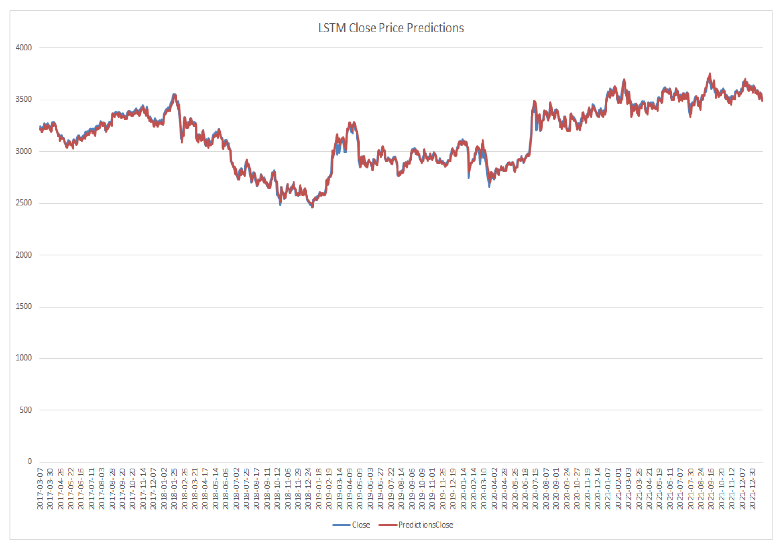
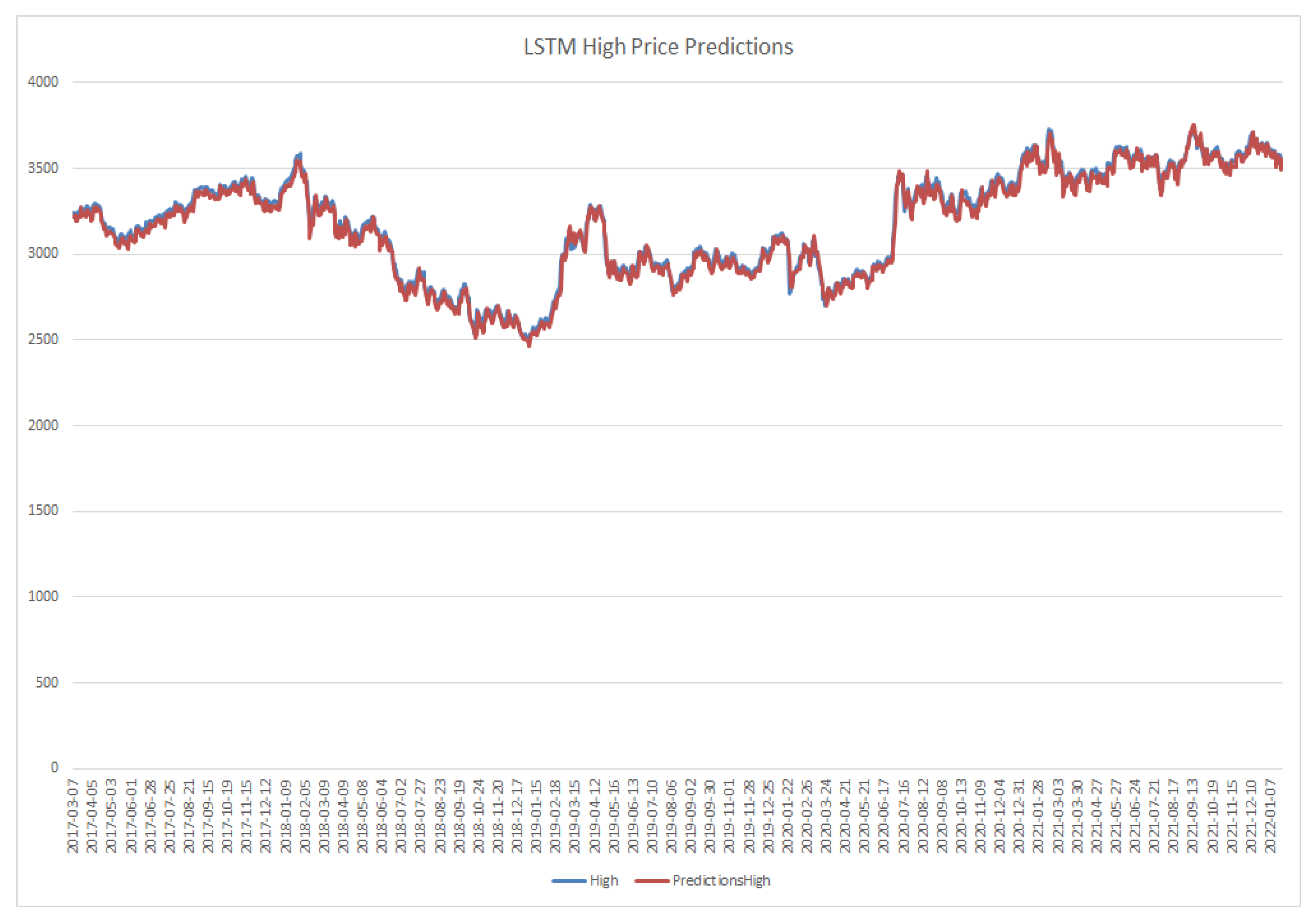
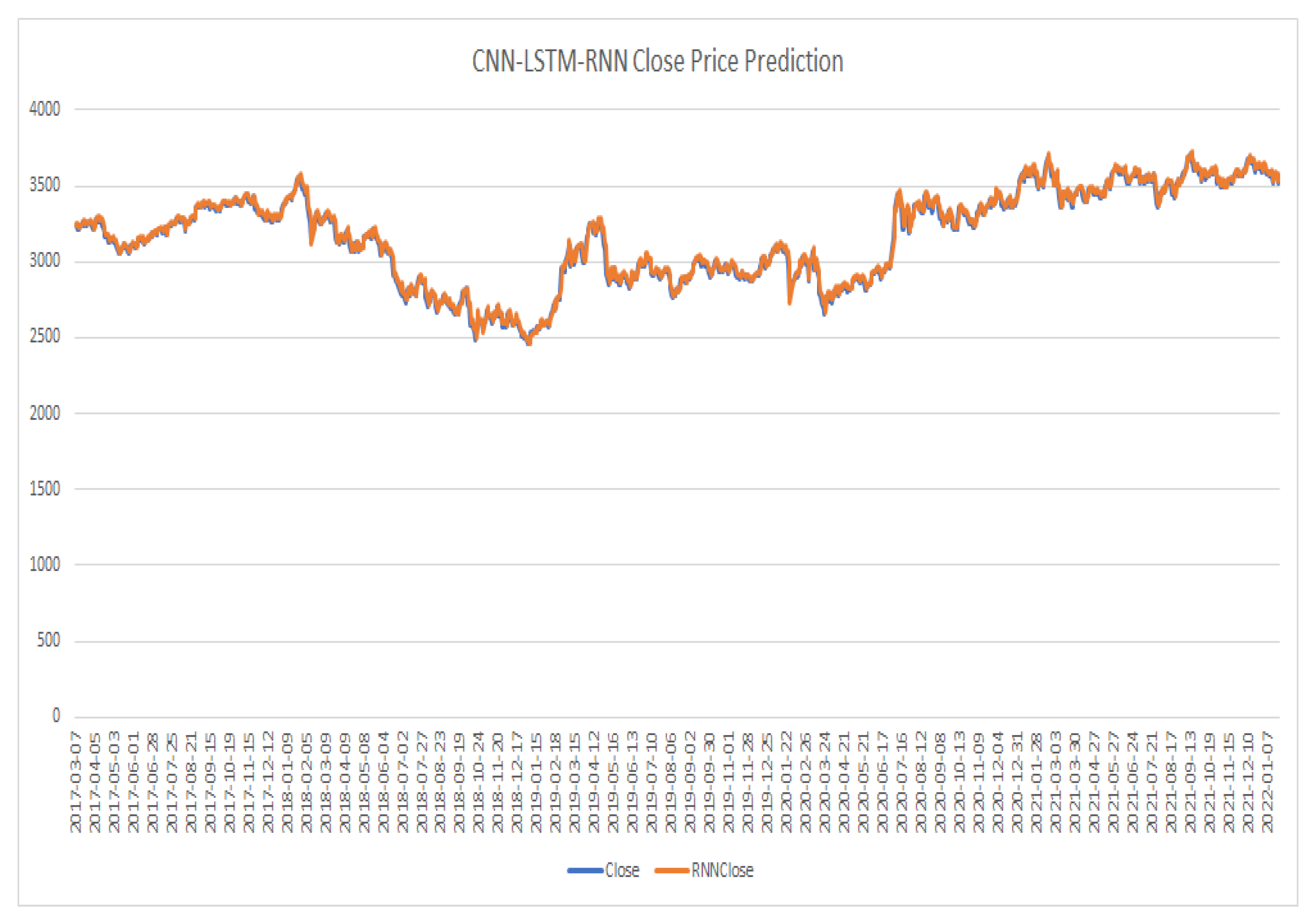
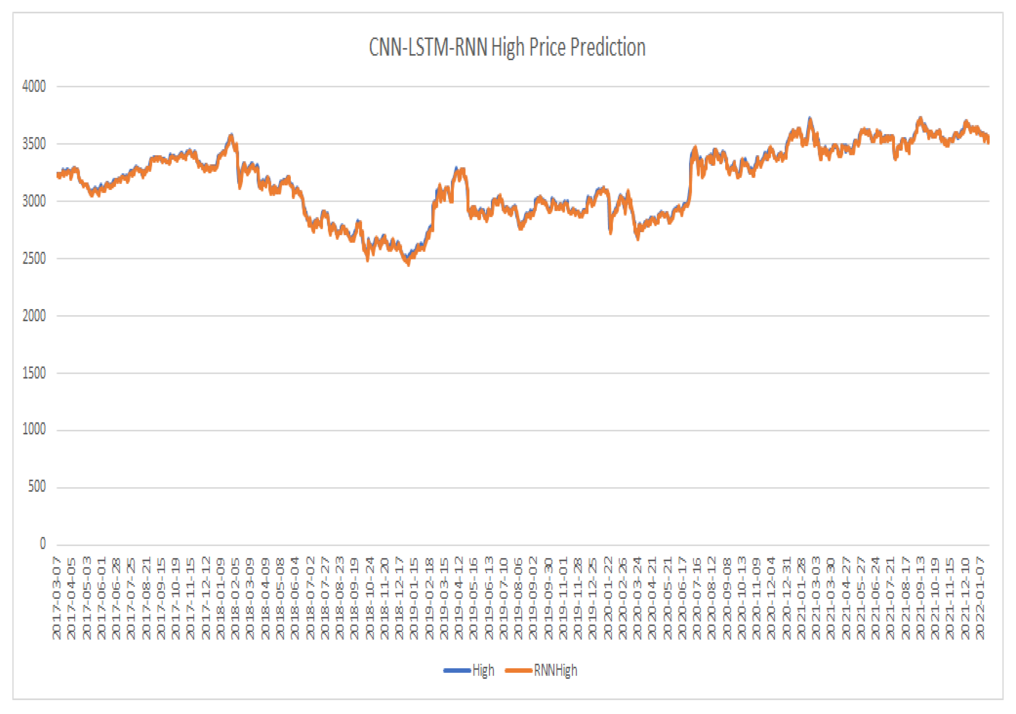
After performing the process to train the existing models CNN, RNN, LSTM, CNN-RNN, and CNN-LSTM are performed on the training data set. After completing the training process, forecasting is performed on the test dataset, which is compared with the actual values as shown in Figure 8, Figure 9, Figure 10, Figure 11, Figure 12, Figure 13, Figure 14, Figure 15, Figure 16, Figure 17, Figure 18 and Figure 19. The line graph of the six forecasting methods presents the actual prices and the forecasted prices. By analyzing the results, the CNN-LSTM-RNN model has the highest line-fitting graph among other models and the CNN model has the lowest.
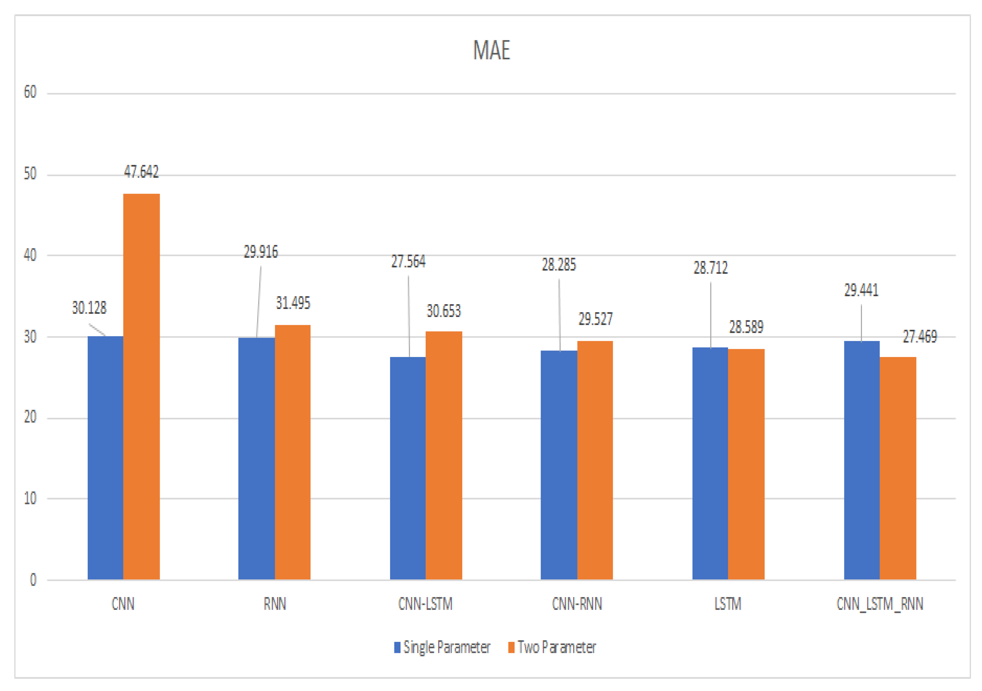
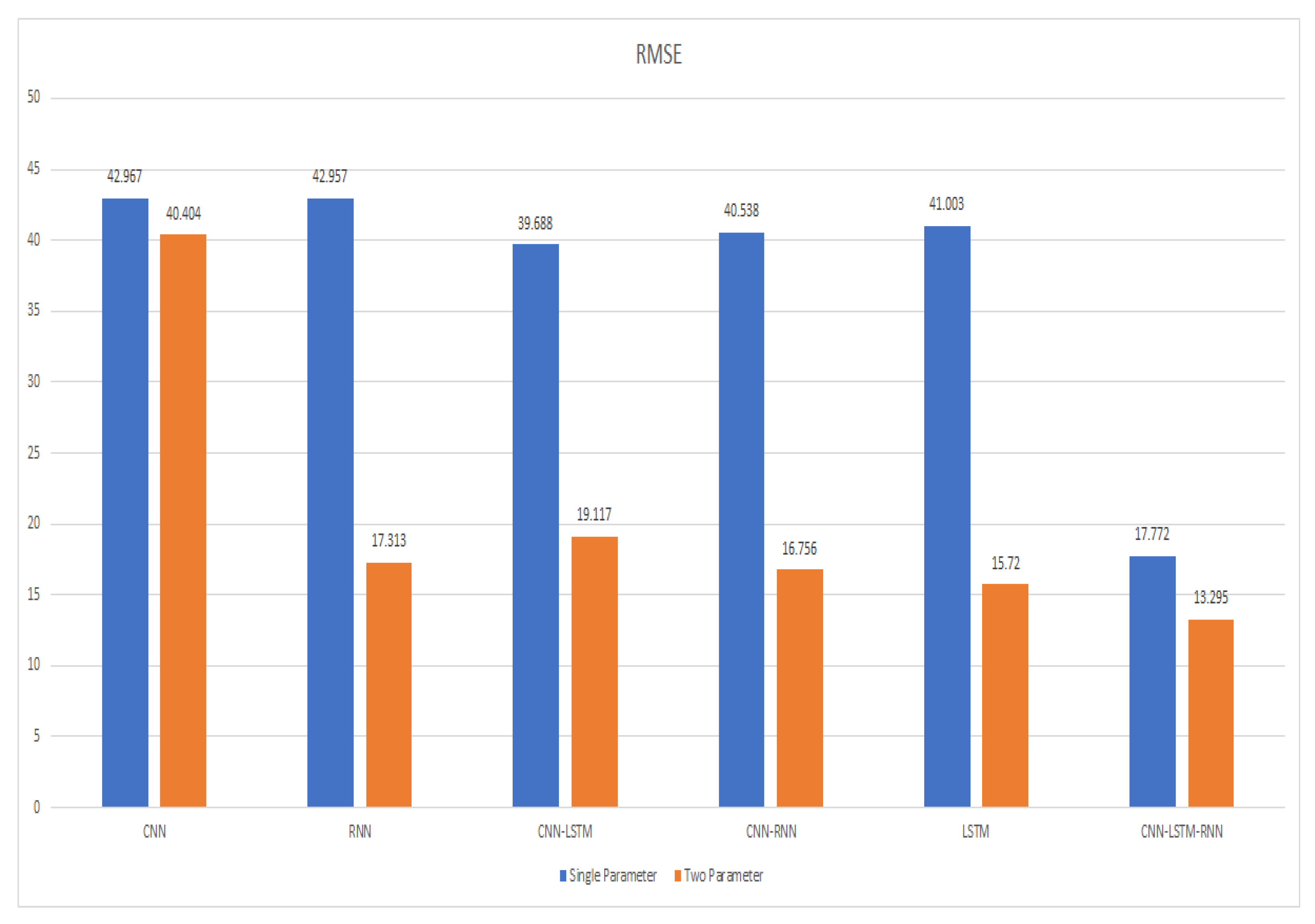
Each method’s evaluation index is also computed. The comparison with other models’ results is displayed in Table 5 and Figure 20, Figure 21 and Figure 22, while CNN-LSTM-RNN has the lowest MAE and RMSE and the R 2 is the greatest and closest to 1 among other models, CNN has the highest MAE and RMSE and the lowest R 2 .
By comparing the RNN with CNN-LSTM, R 2 of CNN-LSTM increases from 0.982 to 0.983 by 0.1%, MAE decreases from 31.495 to 30.653 by 2.7%, RMSE also increases from 17.313 to 19.117 by 10.4%, so the results of CNN-LSTM was better than RNN. Another comparison was conducted between CNN-LSTM and CNN-RNN, and the MAE and RMSE of CNN-RNN decreased, and MAE decreased from 30.653 to 29.527 by 3.8%, and RMSE decreases from 19.117 to 16.756 by 14%, and R 2 increased from 0.983 to 0.984 by 0.1%, so the CNN-RNN performed better than CNN-LSTM. Another comparison was conducted between CNN-RNN and LSTM: MAE of LSTM decreased from 29.527 to 28.589 by 3.4%, RMSE decreased from 16.756 to 15.720 by 6.5%, and R 2 increased from 0.984 to 0.985 by 0.1%, so the LSTM performed better than CNN-RNN. Another comparison was conducted between LSTM and CNN-LSTM-RNN: MAE and RMSE of CNN-LSTM-RNN decreased, MAE decreased from 28.589 to 27.469 by 4%, RMSE decreased from 15.720 to 13.295 by 18%. and R 2 increased by 0.985 to 0.986 by 0.1%, so the CNN-LSTM-RNN performed better than LSTM.
By comparing the proposed technique with existing LSTM technique [14], we see that the previous LSTM approach employed two layers, the first layer consisting of 32 units, and the second layer consisting of 16 units. Another existing RNN technique [11] is compared with the proposed methodology. We see that the existing RNN technique used two layers. In the first layer, six units were used and, in the second layer, 11 units are used, while the proposed technique used a single layer and 64 units in the model.
The main difference with the existing methodologies is that the existing methodologies used the evaluation matrix to check the accuracy of the models, while the proposed techniques select the best model based on R 2 error rate closest to 1. The proposed technique with a single layer and 64 units reduces the computation power and, by increasing the units in the layer, the performance of the model increases and also reduces the error rate. The results verify that the proposed methodology is performing better, and its prediction results are closer to actual prices as compared to the existing LSTM and RNN models. The results of the proposed approach are shown in Table 6.
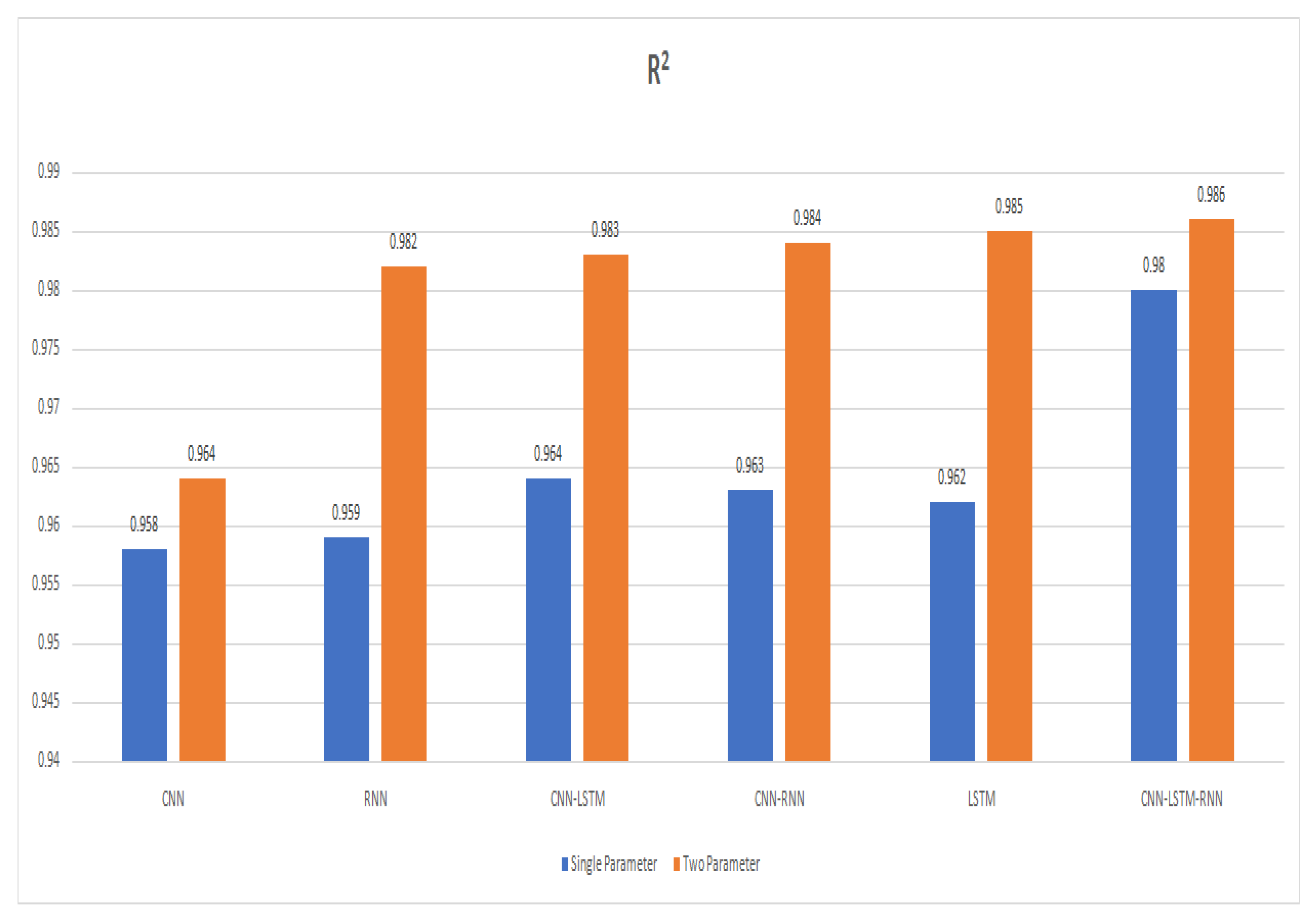
By comparing the error rates results of a single parameter and two parameters, we see that the MAE of the two parameters of CNN, RNN, CNN-LSTM, and CNN-RNN models remains high, whereas the MAE of the LSTM model remains a little bit lower than the then single parameter of the LSTM model. The RMSE of the two parameters is lower than the RMSE of a single parameter. The R 2 error results of two parameters are closest to 1 as compared to the R 2 error result of a single parameter, so the R 2 error results are closest to 1, which means that models with two parameters are performing more accurately as compared to single parameters, as shown in Table 7.
In this study, we have used three regression models, i.e., CNN, LSTM, and single layer RNN. Furthermore, our proposed single layer RNN outperformed as compared to other existing multi-layer and hybrid models shown in Table 5. The proposed single layer RNN model reduces computational complexity as well as significantly reducing RMSE and MAE. In the future, we will extend the comparison parameters, i.e., accuracy, MSE, F1 score, precision, and recall.
By examining the results, we can see that our proposed approach on both scenarios outperforms in comparison to other existing models available in the literature. Besides, by comparing the results of existing single-parameter models with two-parameter models, we see that all the models are performing better on the forecasting of two parameters as compared to the single parameter, which is improved by 0.6%, 0.23%, 0.19%, 0.21%, 0.23%, and 0.6%. In terms of forecasting accuracy the proposed methodology (CNN-LSTM-RNN) of scenario two parameters, the MAE is 27.469, the RMSE is 13.295, and the R 2 is 0.986, which is very close to 1. The highest of the six forecasting approaches, CNN-LSTM-RNN, has a R 2 of 0.986 in the case of high predicting accuracy, which is improved by 2.2%, 0.4%, 0.3%, 0.2%, and 0.1%, respectively.
The technique proposed in this paper is based on CNN, LSTM, and RNN models. The proposed technique outperforms the other five models in forecasting two stock parameters, and the error rate is lower when compared to the other models. This model is forecasting the two stock parameters’ high price and close price for the next day, which will help the investor in investing in the future.

5. Conclusions

In order to forecast the close price and the next day’s high price, in this article we have proposed a single layer RNN model. In addition, our proposed approach leverages the following six input features while utilising all of the time series data. These six features are following: volume, adj-close price, close price, low price, open price, and high price. In our scheme CNN, LSTM, and RNN take the input to performed calculations and forecast the closing and high prices for the following day. Furthermore, in this study, the selection method selects the one model on the basis of evaluation index R 2 , the value which is closest to 1. We have used the Shanghai Composite Index (000001) in this paper to validate the experimental performances of our proposed single layer RNN model with other state of the arts existing multi layer and hybrid schemes. By analyzing the experimental performance, the proposed single layer RNN model outperforms in comparison to other existing models. Our proposed model has the shortest MAE and RMSE as compared to other models as shown in Table 5, while R 2 is the closest to 1. Our proposed single layer RNN model is the suitable model to forecast the stock prices, and it will help the investor to invest in the right stock at right time to gain maximum profit. It only forecasts two stock parameters—close price and high price, respectively, for the next day. In the future, we aim to consider risk factors to make an intelligent decision system and to forecast more than two stock parameters along with evaluation matrix for better results.

Author Contributions

Writing—original draft, S.Z., N.A., S.H., J.I. and S.S.U.; Writing—review & editing, A.D.A. and S.B. All authors have read and agreed to the published version of the manuscript.

Funding

This research is supported by both Princess Nourah bint Abdulrahman University Researchers Supporting Project number (PNURSP2023R51), Princess Nourah bint Abdulrahman University, Riyadh, Saudi Arabia. This work was also supported by the Taif University Researchers Supporting through Taif University, Taif, Saudi Arabia, under Project (TURSP-2020/26).

Data Availability Statement

Not Applicable.

Acknowledgments

The authors would like to acknowledge Princess Nourah bint Abdulrahman University Researchers Supporting Project number (PNURSP2023R51), Princess Nourah bint Abdulrahman University, Riyadh, Saudi Arabia. The authors would like also to acknowledge Taif University Researchers Supporting Project number (TURSP-2020/26), Taif University, Taif, Saudi Arabia.

Conflicts of Interest

The authors declare no conflict of interest.

References

  1. Lu, W.; Li, J.; Li, Y.; Sun, A.; Wang, J. A CNN-LSTM-Based Model to Forecast Stock Prices. Complexity 2020, 2020, 6622927. [Google Scholar] [CrossRef]
  2. Ojo, S.O.; Owolawi, P.A.; Mphahlele, M.; Adisa, J.A. Stock Market Behaviour Prediction using Stacked LSTM Networks. In Proceedings of the 2019 International Multidisciplinary Information Technology and Engineering Conference (IMITEC), Vanderbijlpark, South Africa, 1–22 November 2019; pp. 1–5. [Google Scholar] [CrossRef]
  3. Li, Y.; Pen, Y. A novel ensemble deep learning model for stock prediction based on stock prices and news. Int. Conf. Adv. Comput. Commun. Syst. 2021, 13, 139–149. [Google Scholar] [CrossRef] [PubMed]
  4. Srilakshmi, K.; Sai Sruthi, C. Prediction of TCS Stock Prices Using Deep Learning Models. In Proceedings of the 2021 7th International Conference on Advanced Computing and Communication Systems (ICACCS), Coimbatore, India, 19–20 March 2021; pp. 1–11. [Google Scholar] [CrossRef]
  5. Le, D.Y.N.; Maag, A. Suntharalingam Senthilananthan, Analysing Stock Market Trend Prediction using Machine and Deep Learning Models. In Proceedings of the 2020 5th International Conference on Innovative Technologies in Intelligent Systems and Industrial Applications (CITISIA), Sydney, Australia, 25–27 November 2020; pp. 1–10. [Google Scholar] [CrossRef]
  6. Mehtab, S.; Sen, J. Stock Price Prediction Using Convolutional Neural Networks on a Multivariate Time series. arXiv 2020, arXiv:2001.09769. [Google Scholar] [CrossRef]
  7. Cao, J.; Wang, J. Stock price forecasting model based on modified convolution neural network and financial time series analysis. Int. J. Commun. Syst. 2019, 32, e3987. [Google Scholar] [CrossRef]
  8. Yadava, A.; Jhaa, C.K.; Sharanb, A. Optimizing LSTM for time series prediction in Indian stock market. Procedia Comput. Sci. 2020, 167, 2091–2100. [Google Scholar] [CrossRef]
  9. Lin, B.-S.; Chu, W.-T.; Wang, C.-M. Application of Stock Analysis Using Deep Learning. In Proceedings of the 2018 7th International Congress on Advanced Applied Informatics (IIAI-AAI), Yonago, Japan, 8–13 July 2018; pp. 1–6. [Google Scholar] [CrossRef]
  10. Chen, Y.; Fang, R.; Liang, T.; Sha, Z.; Li, S.; Yi, Y.; Zhou, W.; Song, H. Stock Price Forecast Based on CNN-BiLSTM-ECA Model. Sci. Program. 2021, 2021, 2446543. [Google Scholar] [CrossRef]
  11. Samarawickrama, A.J.P.; Fernando, T.G.I. A Recurrent Neural Network Approach in Predicting Daily Stock Prices. In Proceedings of the 2017 IEEE International Conference on Industrial and Information Systems (ICIIS), Peradeniya, Sri Lanka, 15–16 December 2017; pp. 1–6. [Google Scholar] [CrossRef]
  12. Li, C.; Zhang, X.; Qaosar, M.; Ahmed, S.; Alam, K.M.R.; Morimoto, Y. Multi-factor Based Stock Price Prediction Using Hybrid Neural Networks with Attention Mechanism. In Proceedings of the 2019 IEEE Intl Conf on Dependable, Autonomic and Secure Computing, Intl Conf on Pervasive Intelligence and Computing, Intl Conf on Cloud and Big Data Computing, Intl Conf on Cyber Science and Technology Congress (DASC/PiCom/CBDCom/CyberSciTech), Fukuoka, Japan, 5–8 August 2019; pp. 1–6. [Google Scholar] [CrossRef]
  13. Lounnapha, S.; Zhongdong, W.; Sookasame, C. Research on Stock Price Prediction Method Based on Convolutional Neural Network. In Proceedings of the 2019 International Conference on Virtual Reality and Intelligent Systems (ICVRIS), Jishou, China, 14–15 September 2019; pp. 1–4. [Google Scholar] [CrossRef]
  14. Fabbri, M.; Moro, G. Dow Jones Trading with Deep Learning: The Unreasonable Effectiveness of Recurrent Neural Networks. In Proceedings of the 7th International Conference on Data Science, Technology and Applications, Porto, Portugal, 26–28 July 2018; pp. 1–12. [Google Scholar] [CrossRef]
  15. Prachyachuwong, K.; Vateekul, P. Stock Trend Prediction Using Deep Learning Approach on Technical Indicator and Industrial Specific Information. Information 2021, 12, 250. [Google Scholar] [CrossRef]
  16. Kesavan, M.; Karthiraman, J.; Ebenezer, R.T.; Adhithyan, S. Stock Market Prediction with Historical Time Series Data and Sentimental Analysis of Social Media Data. In Proceedings of the 2020 4th International Conference on Intelligent Computing and Control Systems (ICICCS), Madurai, India, 13–15 May 2020; pp. 1–6. [Google Scholar] [CrossRef]
  17. Batoo, M.; Ghulam, H.; Hayat, M.A.; Naeem, M.; Ejaz, A.; Imran, Z.A.; Spulbar, C.; Birau, R.; Gorun, T.H. How COVID-19 has shaken the sharing economy? An analysis using Google trends data. Econ. Res.-Ekon. IstražIvanja 2021, 34, 2374–2386. [Google Scholar] [CrossRef]
  18. Lecun, S.; Bottou, L.; Bengio, Y.; Haffner, P. Gradient-Based Learning Applied to Document Recognition. Proc. IEEE 1998, 86, 2278–2324. [Google Scholar] [CrossRef] [Green Version]
  19. Lu, W.; Li, J.; Wang, J.; Qin, L. A CNN-BiLSTM-AM method for stock price prediction. Neural Comput. Appl. 2020, 33, 4741–4753. [Google Scholar] [CrossRef]
  20. CNN. Available online: https://www.researchgate.net/figure/An-illustration-of-one-one-dimensional-1D-convolutional-neural-network-CNN-consisting_fig3_333154420 (accessed on 3 March 2022).
  21. Hochreiter, S.; Schmidhuber, J. Long Short-Term Memory Recognition. Neural Comput. 1997, 9, 1735–1780. [Google Scholar] [CrossRef] [PubMed]
  22. LSTM. Available online: https://www.analyticsvidhya.com/blog/2017/12/fundamentals-of-deep-learning-introduction-to-lstm/ (accessed on 4 April 2022).
  23. RNN. Available online: https://www.simplilearn.com/tutorials/deep-learning-tutorial/rnn (accessed on 29 April 2022).
  24. Zhang, H.; Mu, J.-H. A Back Propagation Neural Network-Based Method for Intelligent Decision-Making. Complexity 2021, 2021, 6610797. [Google Scholar] [CrossRef]
  25. Deng, C.; Liu, Y. A Deep Learning-Based Inventory Management and Demand Prediction Optimization Method for Anomaly Detection. Wirel. Commun. Mob. Comput. 2021, 2021, 9969357. [Google Scholar] [CrossRef]
  26. Mehtab, S.; Sen, J.; Dasgupta, S. Robust Analysis of Stock Time Series Using CNN and LSTM-Based Deep Learning Models. In Proceedings of the 2020 4th International Conference on Electronics, Communication and Aerospace Technology (ICECA), Coimbatore, India, 5–7 November 2020; pp. 1–6. [Google Scholar] [CrossRef]
  27. Lee, S.H.; Yoon, S.H.; Kim, H.W. Prediction of Online Video Advertising Inventory Based on TV Programs: A Deep Learning Approach. IEEE Access 2021, 9, 22516–22527. [Google Scholar] [CrossRef]
  28. Ji, X.; Wang, J.; Yan, Z. A stock price prediction method based on deep learning technology. Int. J. Crowd Sci. 2020, 5, 55–72. [Google Scholar] [CrossRef]
  29. Singh, K.; Booma, P.M.; Eaganathan, U. E-Commerce System for Sale Prediction Using Machine Learning Technique. J. Phys. Conf. Ser. 2020, 1712, 012042. [Google Scholar] [CrossRef]
  30. Ananthi, M.; Vijayakumar, K. Stock market analysis using candlestick regression and market trend prediction (CKRM). J. Ambient. Intell. Humaniz. Comput. 2020, 12, 4819–4826. [Google Scholar] [CrossRef]
  31. Parray, I.R.; Khurana, S.S.; Kumar, M.; Altalbe, A.A. Time series data analysis of stock price movement using machine learning techniques. Soft Comput. 2020, 24, 16509–16517. [Google Scholar] [CrossRef]
  32. Mohan, S.; Mullapudi, S.; Sammeta, S.; Vijayvergia, P.; Anastasiu1, D.C. Stock Price Prediction Using News Sentiment Analysis. In Proceedings of the 2019 IEEE Fifth International Conference on Big Data Computing Service and Applications (BigDataService), Newark, CA, USA, 4–9 April 2019; pp. 1–4. [Google Scholar] [CrossRef]
  33. Kumar, D. Stock Forecasting Using Natural Language and Recurrent Network. In Proceedings of the 2020 3rd International Conference on Emerging Technologies in Computer Engineering: Machine Learning and Internet of Things (ICETCE), Jaipur, India, 7–8 February 2020; pp. 1–5. [Google Scholar] [CrossRef]
  34. Sharaf, M.; El-Din Hemdan, E.; El-Sayed, A.; El-Bahnasawy, N.A. StockPred: A framework for stock Price prediction. Multimed. Tools Appl. 2021, 80, 17923–17954. [Google Scholar] [CrossRef]
  35. Zhang, R.; Yuan, Z.; Shao, X. A new combined CNN-RNN model for sector stock price analysis. In Proceedings of the IEEE 42nd Annual Computer Software and Applications Conference (COMPSAC), Tokyo, Japan, 23–27 July 2018; pp. 546–551. [Google Scholar] [CrossRef]
Figure 1. Architecture Diagram.
Mathematics 11 00590 g001
Figure 2. CNN one-dimensional structure [20].
Mathematics 11 00590 g002
Figure 3. LSTM Architecture [22].
Mathematics 11 00590 g003
Figure 4. RNN Architecture [23].
Mathematics 11 00590 g004
Figure 5. CNN Model Diagram.
Mathematics 11 00590 g005
Figure 6. LSTM Model Diagram.
Mathematics 11 00590 g006
Figure 7. RNN Model Diagram.
Mathematics 11 00590 g007
Figure 8. CNN model close price prediction.
Mathematics 11 00590 g008
Figure 9. CNN model high price prediction.
Mathematics 11 00590 g009
Figure 10. RNN model close price prediction.
Mathematics 11 00590 g010
Figure 11. RNN model high price prediction.
Mathematics 11 00590 g011
Figure 12. CNN-LSTM model close price prediction.
Mathematics 11 00590 g012
Figure 13. CNN-LSTM model high price prediction.
Mathematics 11 00590 g013
Figure 14. CNN-RNN model close price prediction.
Mathematics 11 00590 g014
Figure 15. CNN-RNN model high price prediction.
Mathematics 11 00590 g015
Figure 16. LSTM model close price prediction.
Mathematics 11 00590 g016
Figure 17. LSTM model high price prediction.
Mathematics 11 00590 g017
Figure 18. CNN-LSTM-RNN model close price prediction.
Mathematics 11 00590 g018
Figure 19. CNN-LSTM-RNN model high price prediction.
Mathematics 11 00590 g019
Figure 20. MAE comparison between various models.
Mathematics 11 00590 g020
Figure 21. RMSE comparison of multiple different models.
Mathematics 11 00590 g021
Figure 22. R 2 Comparison of different models.
Mathematics 11 00590 g022
Table 2. Shanghai Composite Index (000001) Data Set.
DateOpenHighLowCloseAdj.CloseVolume
03 March 20031511.5841525.6981511.0451525.4831525.4838800
04 March 20031527.4481529.7511517.8591524.3031524.3038000
05 March 20031524.0771524.1231508.250971517.1781517.1786800
06 March 20031516.6001517.3481494.2401498.3431498.3438400
07 March 20031495.6931502.4271489.3841493.0931493.0937000
10 March 20031492.2081496.1631467.6391468.9181468.9187400
12 March 20031468.7461475.2861458.51475.0081475.0085200
13 March 20031475.0361477.8581463.3291464.6491464.6495400
14 March 20031464.9911471.4991461.3501466.0431466.0434800
17 March 20031465.1441469.5321453.3681469.2741469.2746400
Table 3. Model Parameters.
ParametersValues
Convolution Layer1
Convolution Layer Filters32
Convolution Layer Kernel Size1
Convolution Layer Activation Functiontanh
Pooling Layer1
Pooling MethodMax Pooling
Pooling Size2
Strides1
Flatten Layer1
LSTM Layer1
LSTM Layer Units64
LSTM Layer Activation Functiontanh
RNN Layer1
RNN Layer Units64
RNN Layer Activation Function              tanh
OptimizerAdam            
Loss FunctionMAE
Time step10
Batch size64
Epochs100
Table 4. CNN-LSTM-RNN Model Results.
ModelsMAERMSE R 2
CNN27.6443.5270.985
RNN27.46913.2950.986
LSTM32.28320.2420.982
Table 5. Performance evaluation of the suggested approach compared to current techniques.
MethodsMAERMSE R 2
CNN47.64240.4040.964
RNN (Multilayer)31.49517.3130.982
CNN-LSTM(Hybird Model)30.65319.1170.983
CNN-RNN(Hybird Model)29.52716.7560.984
LSTM(Multilayer)28.58915.7200.985
Proposed Single Layer RNN27.46913.2950.986
Table 6. Results of proposed methodology.
Actual Stock PriceProposed Approach
DatesHighClosePredicted HighPredicted Close
07 March 20173242.6589363242.4060063233.8576663242.933838
08 March 20173245.3039553240.6650393237.6086433249.272949
09 March 20173233.8753216.7460943240.6855473254.879883
10 March 20173222.3190923212.760013214.254153224.61792
13 March 20173237.0239263211.5153813211.5153813224.850098
Table 7. Performance comparison of single parameter and two parameter.
Single ParameterTwo Parameter
MethodsMAERMSE R 2 MAERMSE R 2
CNN30.13842.9670.95847.64240.4040.964
RNN(Multilayer)29.91642.9570.95931.49517.3130.982
CNN-LSTM(Hybird Model)27.56439.6880.96430.65319.1170,983
CNN-RNN(Hybird Model)28.28540.5380.96329.52716.7560.984
LSTM(Multilayer)28.71241.0030.96228.58915.7200.985
Proposed Single Layer RNN27.19011.9890.98427.46913.2950.986
Disclaimer/Publisher’s Note: The statements, opinions and data contained in all publications are solely those of the individual author(s) and contributor(s) and not of MDPI and/or the editor(s). MDPI and/or the editor(s) disclaim responsibility for any injury to people or property resulting from any ideas, methods, instructions or products referred to in the content.

