
Viability Selection at Linked Sites

Leibniz Institute for Evolution and Biodiversity, Museum für Naturkunde, Invalidenstraße 43, 10115 Berlin, Germany
Mathematics 2023, 11(3), 569; https://doi.org/10.3390/math11030569
Submission received: 13 December 2022
/
Revised: 16 January 2023
/
Accepted: 18 January 2023
/
Published: 21 January 2023
(This article belongs to the Special Issue Mathematical Models in Evolutionary Ecology)
Abstract
:Evolutionary ecology may be described as explaining ecology through evolution and vice versa, but one may also view it as an integration of the two fields, where one takes the view that ecology and evolution are inseparable, and one can only begin to understand the biology of organisms by synthesizing the two fields. An example of such a synthesis is the biology of high fecundity and the associated concept of sweepstakes reproduction, or skewed individual recruitment success. As an illustration, we consider selection at linked sites under various dominance and epistasis mechanisms in a diploid population evolving according to random sweepstakes and experiencing recurrent bottlenecks. Using simulations, we give a few examples of the impact of the stated elements on selection. We show that depending on the dominance mechanisms, random sweepstakes can shorten the time to fixation (conditional on fixation) of the fit type at all sites. Bottlenecks tend to increase the fixation time, with random sweepstakes counteracting the effects of bottlenecks on the fixation time. Understanding the effect of random sweepstakes, recurrent bottlenecks, dominance mechanisms and epistasis on the fate of selectively advantageous mutations may help with explaining genetic diversity in natural highly fecund populations possibly evolving under sweepstakes reproduction.
Keywords:
high fecundity; random sweepstakes; natural selection; fixation; bottleneck; evolution; ecology; recruitment dynamics; epistasisMSC:
92-04; 92-101. Introduction
Central to understanding the evolution and the ecology and, indeed, the evolutionary ecology of natural populations is recruitment dynamics, i.e., the distribution of individual recruitment success or, in other words, the offspring number distribution. The number of offspring contributed by each individual affects population size and geographic distribution, genetic diversity and the resilience of natural populations [1]. The Wright–Fisher population model of genetic reproduction has been almost universally applied in modeling evolutionary history of natural populations. However, it may be a poor choice for highly fecund populations.
Highly fecund populations provide an important contrast to low fecundity and model organisms, have enormous reproductive potential, are diverse and found widely [1] and may share a key characteristic that is not captured by the Wright–Fisher model, namely, sweepstakes reproduction [2,3]. By “sweepstakes reproduction” we refer to a high variance in individual reproductive success, much higher than is captured by the classical Wright–Fisher model [4]. The population model we apply allows us to define high fecundity without involving sweepstakes reproduction. There are two main forms of sweepstakes reproduction involving different mechanisms turning high fecundity into a skewed individual recruitment success. In one mechanism, referred to as random sweepstakes, Type III survivorship and chance matching of reproduction with favorable environmental conditions, for example in broadcast spawners, combine to form a jackpot of surviving offspring won by a few parents. The other form of sweepstakes reproduction has been referred to as selective sweepstakes [5]. The idea is that potential offspring are viewed as passing through selective filters on their way to maturity, and the surviving offspring have on average a different genetic constitution than the nonsurviving ones; the next time around, another set of types confers advantage [6]. In our formulation, a population may be highly fecund without evolving according to random or selective sweepstakes. Understanding recruitment dynamics in highly fecund populations necessarily centers on identifying sweepstakes reproduction in data and the mechanisms of sweepstakes reproduction, given evidence of it.
Random sweepstakes have been precisely formulated for both haploid and diploid populations [7,8,9,10,11,12,13]. As far as we know selective sweepstakes incorporating high fecundity and random sweepstakes have not been explicitly modeled. An extensive analysis of whole-genome sequences provides evidence for the evolution of the highly fecund diploid Atlantic cod being driven by positive selection [5]. A population model of recurrent sweeps of a new mutation each time, the Durrett–Schweinsberg model [14] essentially explains the Atlantic cod data, while models of random sweepstakes derived for diploid populations [7,15,16] do not, even accounting for complex demography and background selection [5]. In the Durrett–Schweinsberg model [14], the population evolves according to the Moran model of genetic reproduction, where at any given time, one individual is randomly picked to produce one offspring and another individual perishes to keep the population size constant, and so by itself, it does not model high fecundity. To properly take high fecundity into account when modeling selective sweepstakes, where high fecundity is defined as a high reproductive capacity in the absence of selection, one might want, for example, to model recurrent sweeps in a background of random sweepstakes. The main conclusion from the analysis of the Atlantic cod data is that strong pervasive positive selection should be considered in any further analysis of the data. Identifying sweepstakes reproduction in genomic data and resolving the mechanisms of sweepstakes reproduction given evidence of it are two of the main open problems in biology.
To better understand if and how random and selective sweepstakes might interact to shape the evolution of natural populations, it is necessary to illuminate how random sweepstakes affect the fate of advantageous mutations. Here, we use simulations to consider the fate of advantageous types for a simple model of viability selection acting at linked sites in a diploid population evolving according to random sweepstakes and recurrent bottlenecks. With linked sites, we can impose various forms of dominance mechanisms and epistatic interactions between the sites. Similar investigations based on simulations have focused on unlinked sites [17] and a single site [18]. The results indicate that random sweepstakes reduce both the probability of fixation of new advantageous types and the average time to fixation conditional on fixation. We claim that the models of random sweepstakes applied in [17,18], and here as well, have better properties than the original one [10] leading to the multiple-merger Beta-coalescent. Multiple-merger coalescents [9,19,20,21,22], in which a random number of lineages merge each time, arise in different contexts, for example, through a large sample size [23], through recurrent strong bottlenecks [24] or recurrent selective sweeps [14], and may be essential for explaining genetic diversity in natural populations across domains of life [25].
Population models of random sweepstakes and recurrent bottlenecks are in the domain of attraction of jump diffusions and multiple-merger coalescents [24,26]. For an overview of the mathematical formulation of random sweepstakes and the connection to jump diffusions, consult, e.g., [26]. We only draw attention to the SDE
describing the evolution of a type frequency in a haploid population evolving according to random sweepstakes [26]. In Equation (1), is the solution of the SDE in Equation (1) and tracks the frequency of a given type in a haploid population evolving according to random sweepstakes, is a standard Brownian motion, N is a Poisson process on independent of equipped with intensity measure , and F is a finite measure without an atom at zero and corresponds to the random sweepstakes mechanism (the offspring number distribution) [26]. Comparing the probability of fixation of a neutral type evolving according to Equation (1) to one evolving according to the Wright–Fisher diffusion (i.e., ), whose fixation probability is proportional to the initial frequency of the type, would be informative about how the jump term in Equation (1) corresponding to random sweepstakes affects the evolution of the population. In [27], generalized Wright-Fisher models for haploid populations were studied, where
with tracking the number of copies of a given type in a haploid population of fixed size N. The idea was to study a process that matched the Wright-Fisher model only in the first two moments of and without imposing any specific constraints on the higher moments of [27]. Upon adding selection to the generalized Wright–Fisher model, conditions could be identified where a beneficial type fixed with probability one as [27]. Furthermore, [27] identified a continuum limit operator, where
(assuming the absence of mutation), where is a probability measure. Given that a generator as in Equation (3) can be identified, it can be applied, at least in theory, to obtain expressions, e.g., fixation probabilities [27,28]. In our case of a diploid population evolving under random sweepstakes, with random pairing of diploid individuals, identifying a continuum limit operator as in Equation (3) seems far from trivial. Mathematical investigations of the effect of random sweepstakes on selection are restricted to a single site in a haploid population [29,30,31,32]. Considering a model of selection in a haploid population evolving according to random sweepstakes, where the reproduction mechanism is a mixture of “small” and “large” reproduction events [31], Bah and Pardoux studied the SDE
where is standard Brownian and with M taken as a Poisson point measure on with intensity . In [31], Equation (4) is referred to as the -Wright–Fisher SDE with selection. For comparison, the SDE
(simplified to a single population) with denoting the strength of selection is the starting point for investigating the time to fixation (conditional on fixation) in a structured population [33]. Equations (1), (3) and (4) have in common the inclusion of a term due to random sweepstakes, i.e., they are mixtures of a process corresponding to small families (the Wright–Fisher diffusion), and a term corresponding to large families. The model we employ in the simulations (see Section 2) is also composed of such processes.
Our aim is to investigate the joint fixation of a fit type jointly at two or more linked sites in a diploid population evolving according to random sweepstakes and experiencing recurrent bottlenecks. Even though the algorithm developed for the simulations works for any number of sites, the number of possible phased L-site types increases exponentially with L, and thus there are computational restrictions (e.g., amount of computer memory) to how many sites can be included. This may not be much of a restriction, however, since adaptation may mostly be due to few new mutations each of large effect [34,35]; this has been referred to as the oligogenic model [36].
In Section 2, we describe the model we apply in the simulations, in Section 3, we present and discuss the results, in Section 4, we briefly summarize the results and remaining open problems, in Appendix A, we present further simulation results and in Appendix B, we provide an overview of the simulation algorithm in the form of a pseudocode.
2. Materials and Methods
We consider a diploid population evolving in discrete (nonoverlapping) generations. In any given generation, the current individuals randomly form pairs, the pairs independently produce potential offspring (juveniles), and from the pool of juveniles, we sample a specified number who will survive and produce a new set of reproducing individuals. Thus, we are essentially modeling a supercritical multitype branching process, which is at times conditioned to be at a given value. Incorporating potential offspring into our model allows us to formulate the concepts of high fecundity and sweepstakes reproduction. We define high fecundity as the ability of organisms to produce numbers of juveniles at least on the order of the population size. In our formulation, high fecundity is a necessary but not sufficient ingredient for sweepstakes reproduction to occur; what is missing is a mechanism turning high fecundity into sweepstakes reproduction. Here, we take sweepstakes reproduction to refer to a high variance in individual reproductive output. One such mechanism is random sweepstakes, whereby Type III survivorship and chance matching of reproduction with favorable environmental conditions, for example among marine broadcast spawners, combine to generate a jackpot so that a few individuals produce the bulk of the surviving offspring. This mechanism has previously been referred to as sweepstakes reproduction [2,3]. Natural selection is not involved in random sweepstakes, but is a key player in another conceptual mechanism turning high fecundity into sweepstakes reproduction, selective sweepstakes [5,6].
Now we formulate random sweepstakes. Our formulation is based on the haploid population model of random sweepstakes in the domain of attraction of the Beta-coalescent for [10]. Let for denote i.i.d. copies of positive random variables, where denote the independent and identically distributed random number of juveniles produced by M parent pairs (randomly formed) in a given generation. Note that our formulation of randomly forming pairs of parents is in contrast to some models involving “diploid” populations. Sometimes, the only notion of diploidy is to assume an even number of individuals (population size ), and the actual mechanism in the model is more often than not strictly haploid (e.g., [14]). Take
where and C are positive constants. Before we explain where Equation (5) comes from, we add the following. For the simulations, we take without loss of generality and choose and C so that
and is an upper bound on the number of juveniles. The limiting coalescent (i.e., a coalescent is a probabilistic description of the random ancestral relations of sampled gene copies from a hypothetical population evolving according to a given population model, e.g., Equation (5)) is being investigated for a planned future publication. One can argue that the assumption where K is a positive constant is biologically realistic. The juveniles represent fertilized eggs, and it is plausible, in particular for marine broadcast spawners, that the number of fertilized eggs produced even over the lifetime of a given individual is at most a fraction of the population size. The cutoff also provides a means of formally defining a highly fecund population. A population evolving according to Equation (5) is taken to be highly fecund if as . The model in Equation (5) is a variant of the model in [10] where, with a normalizing constant, the law for the random number of juveniles (X) produced by a given individual behaves as
The model in Equation (6) is defined in terms of the tail probability . The corresponding tail probability for Equation (5) is . Note that . The formulation in Equation (5) is in terms of the mass function to guarantee that the mass function is monotonically decreasing as k increases , when an upper bound on X is applied. Thus, the model in Equation (5) is a natural way of modeling random sweepstakes, where the number of juveniles produced by each individual is random. The model is realistic in the sense that we give each individual (or pair of individuals) the capacity to produce a large enough number of juveniles to impact the population without asking for unrealistic numbers as is being done in Equation (6). The random gene genealogy of a sample of gene copies from a haploid population evolving according to Equation (6) is described by a discrete-time -coalescent (admitting simultaneous multiple mergers of ancestral lineages) in the case , by the Beta-coalescent when and if , one obtains the Kingman coalescent [10]. Thus, one may describe a population evolving according to Equation (5) as evolving according to random sweepstakes if and the cutoff is at least on the order of the population size. In addition to being a natural model of random sweepstakes, the model in Equation (5) also serves as a natural, biologically realistic and a mathematically tractable alternative to the Wright–Fisher model. Given our formulation, a highly fecund population may or may not evolve according to random sweepstakes.
For the ancestral process describing the random ancestral relations of sampled gene copies from a haploid population evolving according to Equation (6) converges (in the sense of convergence of finite-dimensional distributions) to a multiple-merger coalescent with time measured in units of generations [10]. However, recovering the observed number of mutations in a sample becomes problematic for estimates of close to one [18]. One way to get around this difficulty may be to assume a simple mixture distribution on in Equation (5). Fix and . Suppose with probability , we take , and with probability , we take . In this way, we model random sweepstakes in a broadcast spawner, where most of the time (i.e., with probability ) individuals produce a small number of juveniles (through ), but occasionally reproduction matches favorable environmental conditions so that individuals have an increased chance of producing a large number of juveniles (through ). Thus, we can write, with denoting the law in Equation (5) for given and ,
Similar mixture models of random sweepstakes as described in Equation (7) have been shown to yield nontrivial limits with less problematic scaling of time [11,37]. We claim that a scaling of can be obtained so that the ancestral process converges to a nontrivial limit (the details are being worked out for a planned future publication). A similar mechanism based on the Moran model, where a single parent produces a fixed number ( for some fixed ) of surviving offspring with probability and one offspring with probability , leads to a mixture of a Kingman coalescent and a multiple-merger coalescent [11] (see also [37] for a more thorough investigation of the resulting coalescents derived from a Moran model extended in this way). Each juvenile inherits gene copies according to Mendel’s laws; we exclude mutation.
If the total number of juveniles produced in any given generation exceeds a fixed carrying capacity , viability selection kicks in. We assume the environment can sustain at most diploid individuals. Given the phased genome of a juvenile, we compute the weight as in Equation (8) for some given weight function f. For each given juvenile, a random exponential is then sampled with, as its rate, the viability weight of the juvenile. The juveniles with the smallest realized exponentials (in case the total number of juveniles exceeds ) survive to form the next generation of reproducing individuals. This is a way of using viability selection to sample the juveniles. The probability of surviving generally increases with the number of copies of the fit type one carries. The exact configuration of the types in any given juvenile may also play a role. When , all the juveniles survive. Viability selection only kicks in when the number of juveniles exceeds the carrying capacity. Under recurrent bottlenecks, the population may evolve neutrally for periods of time when recovering from a bottleneck.
In any given generation a bottleneck occurs with a fixed probability b. When a bottleneck occurs, a fixed number B of individuals are sampled uniformly and without replacement to survive the bottleneck and produce juveniles. Clearly, it would be more realistic to sample a random number of juveniles to survive a bottleneck; however, we elect to keep b and B constant. The population size at time is then given by
where M is the number of individuals in generation t available for (randomly) forming parent pairs producing juveniles,
In the total absence of bottlenecks , viability selection acts in every generation (recall Equation (5)). In the presence of bottlenecks , the population evolves neutrally after a bottleneck occurred until the number of juveniles exceeds the carrying capacity. In Appendix B, we describe the algorithm for the simulations.
Throughout, let L denote the number of linked sites. At each site, there are two types, a wild type, or the type already present in the population, and a fit type arising by mutation and conferring advantage. Let denote the set of all possible phased L-site types. We define a viability weight for a juvenile with genome as the map
where is the strength of selection and f is a weight function . To give an example, let us write a genome G as for the genotypes at the L sites, where zero stands for homozygous for the wild type , one for the heterozygous state and two for the homozygous state for the fit type . For example, writing if A holds and zero otherwise, we can take the weight function f from Equation (8) as
where we add one to the value of the weight function if the fit type is found in a homozygous state at a site for each site; in other words, the fit type is recessive at all the sites (see Figure 1). In Equation (9), we exclude epistasis. A juvenile with a genotype of all wild types (i.e., homozygous for the wild type at all sites) will (in general) be assigned a weight of one, thus forming a baseline fitness value.
Considering two sites and assuming at which site a fit type occurs is irrelevant, we have the following seven configurations; with denoting a haplotype with type a at site one and type b at site two, we have the configurations , , , , , , and . In this notation, configuration means haplotypes and and genotypes at site one and at site two.
Fully taking into account the phase between two sites yields sixteen possible genomic configurations ( if L sites), where the possible haplotypes are , , , and . The possible configurations are shown in Table 1, where the entries are examples of the values of the weight function , with denoting the two haplotypes.
To put our model in context, the effect of sites on an additive trait with trait value z was formulated as
where is the genotype at site ℓ, is a map for translating the given genotype into a contribution to the trait value and is the effect of site ℓ on the trait value [38]. The formulation in Equation (10) corresponds to our weight function f in Equation (8). Quite often a so-called Gaussian fitness is then assumed with the fitness computed according to
where denotes the optimal trait value and s the strength of selection [38]. Then, the formulation in Equation (11) corresponds to our map in Equation (8).
3. Results
Let denote the frequency of the fit type at site ℓ at time t and let us write, for any ,
for some given starting frequency . In the simulations, we start with the fit type in one copy at each site, i.e., L individuals are heterozygous at a single site, and homozygous for the wild type at all other sites, and . We define “fixation” as the event . If the fit type is lost at any site, fixation by definition cannot occur. Given the definition of , we can define the probability of fixation at L sites and the expected time to fixation conditional on fixation
A mathematical investigation of or would necessarily have to consider the L-dimensional process since one would need to keep track of the number of copies of the fit type at all sites. Here, we do not aim for precise estimates of or , but only give a few examples of how random sweepstakes, recurrent bottlenecks, dominance mechanisms and epistasis affect the statistics. The fixation probability carries both historical and practical weight, as it can inform about adaptation, loss of genetic variation and the speed of emergence of the resistance to antibiotics among pathogens [39]. The time to fixation (conditional on fixation) is also important [40]. A strongly advantageous type in a single population evolving according to the Moran model takes on the order of time units to fix (given it will fix) on average [14]; in a structured population the time to fixation depends on the migration rate between the subpopulations [33].
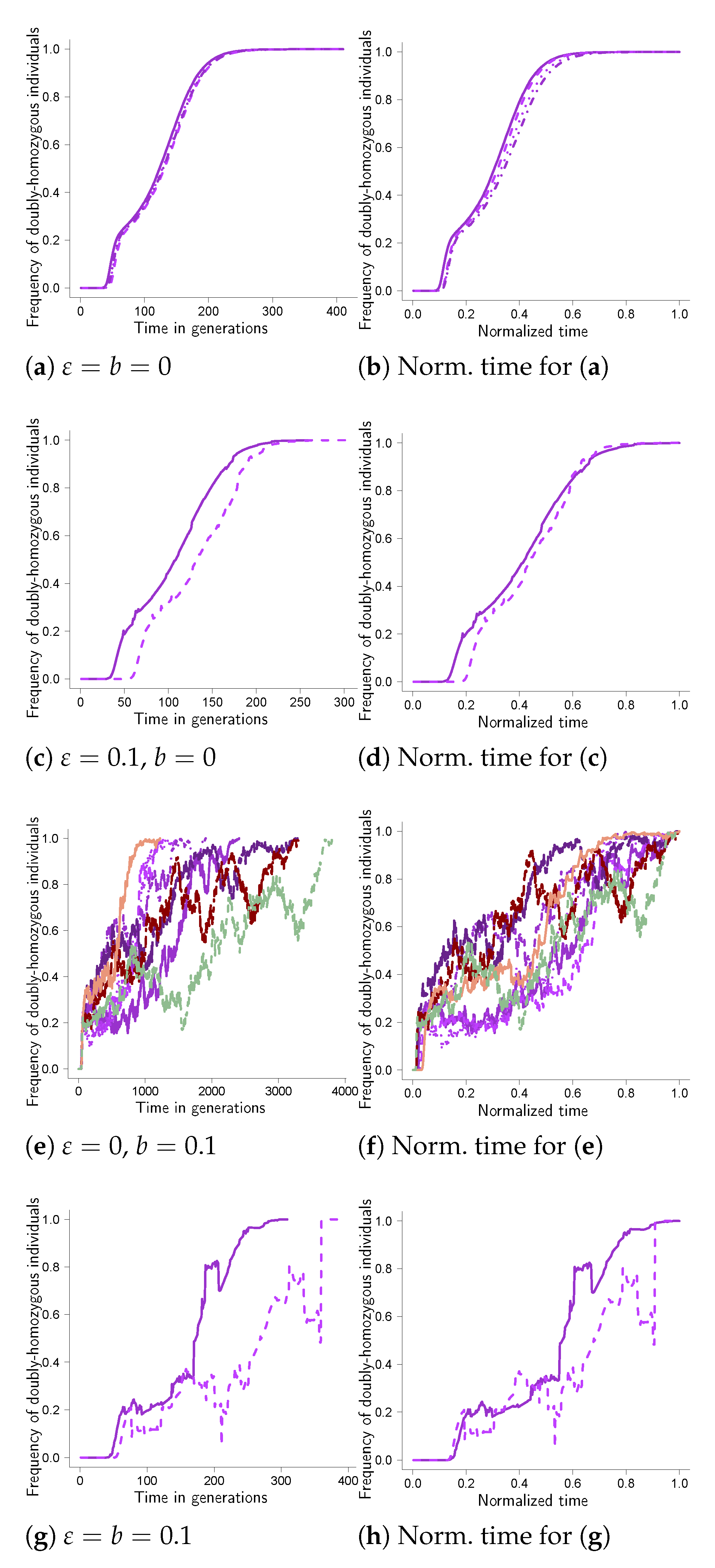
Figure 1 records examples of excursions to fixation at two linked sites with the weight function given by Equation (9). In Equation (9), the weight function increases by one if the fit type is found in a homozygous state at a site; there is no epistasis. In all graphs of fixation trajectories (Figure 1 and Figure A1, Figure A2, Figure A3, Figure A4, Figure A5, Figure A6, Figure A7, Figure A8 in Appendix A) the trajectories in each panel were all obtained under identical conditions. We also remark that the scale of the abscissa (time axis) may differ between panels in each figure. The panels record the excursions for (the probability of taking in Equation (5)) and b (the probability of a bottleneck in any given generation) as shown. The excursions in Figure 1 are shown as the number of diploid individuals homozygous for the fit type at both sites relative to the population size as a function of time. The panels in the right column (b, d, f and h) record the corresponding trajectories in the left column (a, c, e and g) with the time of each trajectory normalized by the time to fixation for the trajectory so that each trajectory reaches the value one at time one. A fixation trajectory for a single mutation with selective advantage has been described as consisting of “phases”, with the phase in which the mutation sweeps from a “low” () frequency to a “high” frequency lasting on the order of generations [41]. The estimate, coupled with the approximation for the average time it takes a mutation to sweep in a population evolving according to the Wright–Fisher model necessarily requires . In Figure 1a, we see that it takes roughly 300–400 generations for a mutation to fix in the absence of random sweepstakes, which matches reasonably well with the estimate of the time to fixation conditional on fixation for a single mutation in a diploid population evolving according to the Wright–Fisher model [42], even though in our case, the trajectories represent the joint fixation at two sites. In Figure 1a, we also see that the time it takes the trajectory to increase from a “low” to “high” frequency is roughly 100 generations, or around tenfold the estimate given in [41].
The logistic differential equation
has been applied in describing how an advantageous type at a single site with selective advantage s increasing in frequency in a population during a sweep [43]. A different approach based on random partitions governed by a stick-breaking construction has also been investigated [44]. In our case, with multiple (at least two) sites, we suggest extending the random partitions approach of [44] (see also [45]) to incorporate multiple sites might be feasible. We are interested in investigating how well fixation trajectories tracing the joint fixation at two or more sites compare to the sigmoidal shape predicted by Equation (13) traditionally used to describe fixation trajectories. The shape of the trajectories in Figure 1 is clearly not captured by Equation (13). An extensive analysis of genomic data from Atlantic cod indicates that strong positive selection is pervasive, leading to a convex (or U-shaped) site-frequency spectrum being consistently observed throughout the genome. Suppose that many of the mutations observed in a U-shaped site-frequency spectrum are selectively advantageous mutations traveling along a fixation trajectory. Then, we would like to understand if a particular shape of a fixation trajectory predicts a U-shaped site-frequency spectrum and another particular shape not. Knowing the potential correspondence between the shape of a fixation trajectory and the shape of a site-frequency spectrum may also inform about the likely dominance mechanism of positive mutations.
The trajectories in Figure 1a (and hence also those in Figure 1b) are from ten experiments, and in all other panels, from one hundred () experiments; thus, random sweepstakes and recurrent bottlenecks reduce somewhat. We emphasize that we are not aiming for precise estimates of or defined in Equation (12). Bottlenecks in the absence of random sweepstakes clearly tend to increase the time to fixation (Figure 1e), with the effect of bottlenecks on the time to fixation negated by random sweepstakes (Figure 1g). In our framework, we keep the cutoff in Equation (5) fixed at the carrying capacity. When a bottleneck occurs the population size is reduced to some given value, which is less than the carrying capacity. The individuals producing juveniles right after a bottleneck do so with the cutoff higher than the current population size, resulting in individuals having a higher chance of producing a large (relative to the current population size) number of juveniles. Simulation results have shown that increasing the cutoff relative to the population size reduces the fixation time (conditional on fixation) [46]. In Figure 1c, we see little effect of random sweepstakes on the time to fixation in the absence of bottlenecks; we claim this is due to taking the cutoff the same as the population size, or the carrying capacity in this case.
Normalizing the time to fixation (Figure 1b,d,f,h where the time to fixation for each trajectory is normalized by the time to fixation for the trajectory) informs about the time spent in each “phase” of the trajectory. The normalized trajectories (dimensionless in time) show the cumulative proportions of each particular realization’s time to fixation. For example, in Figure A2b, the time to fixation is clearly dominated with the fit type at high frequencies at both sites. In contrast, in Figure 1b, the trajectory is increasing essentially linearly from low to high frequencies and in doing so spends around of the time to fixation at “intermediate” frequencies. Given the estimate stated in [41], a type taking on average of order generations to travel to fixation should then be spending on average about of the time to fixation in “intermediate” frequencies. For and , this is around .
Further examples of fixation trajectories are given in Figure A1, Figure A2, Figure A3, Figure A4, Figure A5, Figure A6, Figure A7, Figure A8 in Appendix A. Comparing the results for the given weight functions reveals that there are two main patterns. One pattern is the one in Figure 1, which is essentially mirrored in Figure A1, Figure A4, Figure A5, Figure A7 and Figure A8. In Figure A1, we took the weight function as in Equation (A1), as in Equation (A4) for Figure A4, in Equation (A5) for Figure A5 and as in Equation (A4) for Figure A7 and Figure A8. In Figure A7, we took , and in Figure A8, we took , the other parameter values being the same.
The other pattern is represented in Figure A2 and Figure A3 (both for two sites), and in Figure A6 (for three sites). Taking the weight function as in Equation (A2) yields the results in Figure A2, in Equation (A3) the results in Figure A3 (two sites) and in Figure A6 (three sites). In this pattern the trajectories without random sweepstakes or bottlenecks (Figure A2a) have the shape of a completely dominant type at a single site (see e.g., [18]), although the weight function (Equation (A2) resembles one for a recessive type. In addition, random sweepstakes clearly shorten the time to fixation in the absence of bottlenecks (e.g., Figure A6c), and counteract the effect of bottlenecks on the time to fixation (conditional on fixation; e.g., Figure A7g).
4. Discussion
We gave examples of the joint effects of random sweepstakes, recurrent bottlenecks and dominance mechanisms on the fate of selectively advantageous mutations at linked sites. We showed that, depending on the dominance mechanism, random sweepstakes could shorten the time to fixation (conditional on fixation at all the sites). Bottlenecks could increase the fixation time, and random sweepstakes counteracted the effect of bottlenecks on the fixation time regardless of the dominance mechanism. The shape of the fixation trajectories could be broadly divided into two categories in the absence of bottlenecks, one with a linear increase from “low” to “high” frequencies and another where the trajectories spent nearly the whole time with the fit type in high frequencies at all sites. We emphasize that we did not aim for precise estimates of the probability of fixation or the time to fixation (conditional on fixation) or to investigate many possible scenarios. However, our algorithm provided a tool for further investigations of various demographic and molecular mechanisms on selection. Similar results on the interaction between bottlenecks and random sweepstakes have been obtained for selection acting at a single site [18] and unlinked sites [17].
Studies of selection acting at more than one site generally focus on how a trait value affected by the sites evolves, in particular in reference to a given optimum (e.g., [38]). The effects of the sites on the trait value may vary, and some studies have investigated the evolution of a trait given a change in the optimum when the trait value is determined by many sites (or loci) [47,48]. Our simulation algorithm can, in principle, handle any number of linked sites. However, in particular given that we need to keep track of the number of copies of the fit type at all sites, there are practical considerations (for example computer memory) that limit the number of sites that in practice can be considered. In addition, adaptation may be at least to a large degree due to a few genes of major effect [36].
Our algorithm keeps track of phased haplotypes, so we can investigate the effect of epistasis on selection. Epistasis may be a key player in adaptation [49,50,51]. Significant amounts of genetic variation despite pervasive strong selection may indicate that there is considerable amount of “genetic constraints” [52]. Maybe selection acting on two or more sites with epistatic interactions between the sites can be a way of incorporating genetic constraints.
Evolution can occur “rapidly”, as many examples from nature show [53,54,55,56,57,58]. Our results showed that the joint fixation at two or more sites occurred on a timescale comparable to , the order of time it took a sweep of a single beneficial mutation of advantage s to complete. Understanding the time to fixation at two or more sites may be important in the battle against antibiotic and pesticide resistance [59,60,61].
An open problem is rigorously verifying the simulation results. Here, multitype branching process theory [62,63,64,65,66,67] may be useful. The mathematical analysis of the model of random sweepstakes given in Equation (7) and applied in the simulations is ongoing. There is also a need for further mathematical theory for inferring evolutionary histories of natural populations, in particular in view of the results of [5]. There may be a high cost of selection in populations evolving according to recurrent selective sweepstakes [68]. We anticipate that models of random sweepstakes incorporating strong positive selection in the form of recurrent selective sweeps of strongly advantageous types arising by mutation will be necessary for understanding high fecundity. In particular, high fecundity and random sweepstakes might enable populations to “pay for selection”, i.e., withstand the cost of strong pervasive positive selection.
Funding
This research was funded by Deutsche Forschungsgemeinschaft (DFG)—Projektnummer 273887127 through DFG SPP 1819: Rapid Evolutionary Adaptation grant STE 325/17 to Wolfgang Stephan; acknowledge funding by the Icelandic Centre of Research (Rannís) through an Icelandic Research Fund Grant of Excellence no. 185151-051 to Einar Árnason, Katrín Halldórsdóttir, Alison M. Etheridge, Wolfgang Stephan and BE. BE also acknowledges Start-up module grants through SPP 1819 with Jere Koskela, Maite Wilke-Berenguer and with Iulia Dahmer.
Data Availability Statement
The CWEB (C++) code written for the simulations is available at https://github.com/eldonb/fixation_many_sites (accessed on 13 December 2022).
Acknowledgments
We thank three anonymous reviewers for helpful comments and suggestions.
Conflicts of Interest
The authors declare no conflict of interest. The funders had no role in the design of the study; in the collection, analyses, or interpretation of data; in the writing of the manuscript; or in the decision to publish the results.
Appendix A
In this section, we give further examples of fixation trajectories (Figure A1, Figure A2, Figure A3, Figure A4, Figure A5, Figure A6, Figure A7, Figure A8) for various weight functions. Throughout, the viability weight was computed as in Equation (8). In each graph, a trajectory to fixation traces, as a function of time, the number of diploid individuals homozygous for the fit type at all sites relative to the population size (the number of diploid individuals). Throughout, we considered viability selection acting at linked sites in a diploid population evolving according to Equation (7) with and and the cutoff in Equation (5) set to the carrying capacity . Every time, we started with the fit type in a single copy at each site for all sites. Furthermore, each diploid individual was heterozygous at most at one site to begin with, i.e., at the start, each individual carried at most one copy of a fit type. The algorithm is given as a pseudocode in Appendix B.
Let for denote haplotype i (arbitrarily labeled) in a given juvenile. In Figure A1, we record examples of excursions to fixation at two sites with the weight function (recall the definition of a viability weight in Equation (8)) given by
and recall that we denote a genome by G. Compare Equation (A1) with Equation (9). In Equation (A1), the value of the weight function increases by one for each haplotype carrying the fit type at all sites.
Figure A2 records examples of excursions to fixation at two sites for the weight function
The idea behind the mechanism in Equation (A2) is to model essentially a recessive fit type; however, the excursions in Figure A2a resemble the ones for a dominant type.
In Figure A3, with a weight function for two sites given by (with for denoting haplotype i, arbitrarily labeled, in a given juvenile)
The weight function in Equation (A3) takes the value one if and only if at least one of the two haplotypes in a given juvenile carries the fit type at all sites. In Figure A6, we record fixation trajectories for three sites with the weight function given by Equation (A3).
Figure A4 records trajectories for two sites when the weight function is of the form
In Equation (A4), a juvenile homozygous for the fit type at all sites has maximum fitness, but having one haplotype carrying only a fit type brings disadvantage if the other haplotype does not follow suit. In Figure A7 and Figure A8, we record fixation trajectories for three sites with weight function as in Equation (A4) and in Figure A8, with .
In Figure A5, we record fixation trajectories for three sites with weight function given by
In Equation (A5), the weight function in Equation (8) takes the value one if a juvenile is homozygous for the fit type at all three sites, otherwise the value zero.
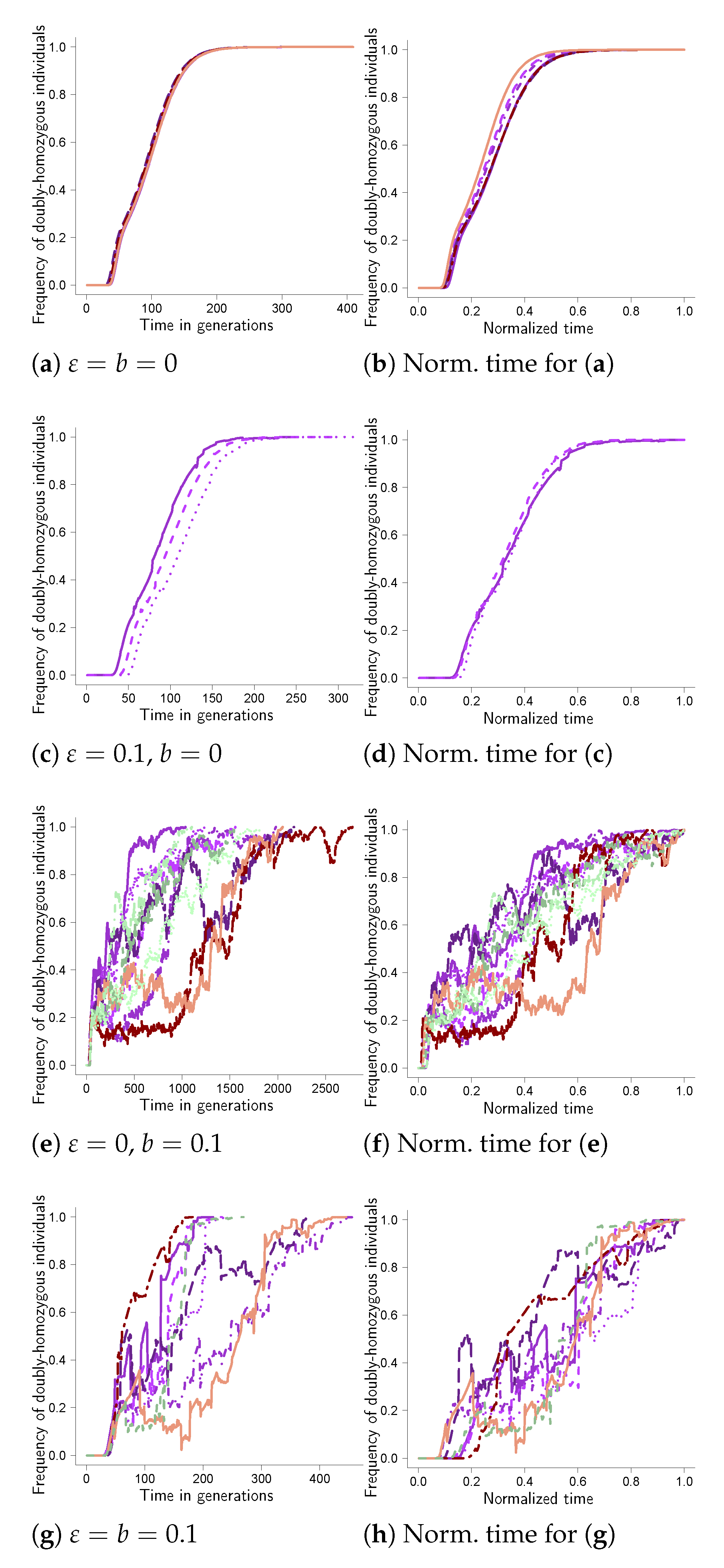
Figure A1.
Two sites with weight function as in Equation (A1). Examples of trajectories to fixation at two sites with weight determined by Equation (8) with weight function as in Equation (A1) for carrying capacity , cutoff , probability of recombination between adjacent sites, , , (see Equation (7)) and probability of a bottleneck b as shown, strength of selection and bottleneck . Each panel shows the trajectories from ten experiments for (a,b) otherwise from experiments. Each trajectory traces, as a function of time, the number of diploid individuals homozygous for the fit type at all sites relative to the population size (the number of diploid individuals). The panels on the right (b,d,f,h) show the corresponding excursions from the left panels (a,c,e,g), where the time to fixation for each excursion is normalized by the time to fixation for the excursion. The scale of the abscissa (time axis) may vary between panels; in each panel the trajectories were all obtained under identical conditions.

Figure A2.
Two sites with weight function as in Equation (A2). Examples of trajectories to fixation at two sites with weight determined by Equation (8) with weight function as in Equation (A2) for carrying capacity , cutoff , probability of recombination between adjacent sites, , , (see Equation (7)) and probability of a bottleneck b as shown, strength of selection , bottleneck and results out of ten experiments for (a); experiments for (c); experiments for (e,g). Each trajectory traces, as a function of time, the number of diploid individuals homozygous for the fit type at all sites relative to the population size (the number of diploid individuals). The panels on the right (b,d,f,h) show the corresponding excursions from the left panels (a,c,e,g), where the time to fixation for each excursion is normalized by the time to fixation for the excursion. The scale of the abscissa (time axis) may vary between panels. In each panel, all the trajectories were obtained under the same conditions.

Figure A3.
Two sites with weight function as in Equation (A3). Examples of excursions to fixation at two sites with weight function as given by Equation (A3) for carrying capacity , cutoff , probability of recombination between adjacent sites, , , (see Equation (7)) and probability of a bottleneck b as shown, strength of selection , bottleneck and results out of ten experiments for (a); otherwise experiments. Each trajectory traces, as a function of time, the number of diploid individuals homozygous for the fit type at all sites relative to the population size (the number of diploid individuals). The panels on the right (b,d,f,h) show the corresponding excursions from the left panels (a,c,e,g), where the time to fixation for each excursion is normalized by the time to fixation for the excursion. The scale of the abscissa (time axis) may vary between panels; in each panel, the trajectories were all obtained under identical conditions.

Figure A4.
Two sites with weight function as in Equation (A4). Examples of excursions to fixation at two sites with weight function as given by Equation (A4) for carrying capacity , cutoff , probability of recombination between adjacent sites, , , (see Equation (7)) and probability of a bottleneck b as shown, strength of selection and bottleneck ; results from ten experiments for (a,c); otherwise, from experiments. Each trajectory traces, as a function of time, the number of diploid individuals homozygous for the fit type at all sites relative to the population size (the number of diploid individuals). The panels on the right (b,d,f,h) show the corresponding excursions from the left panels (a,c,e,g), where the time to fixation for each excursion is normalized by the time to fixation for the excursion. The scale of the abscissa (time axis) may vary between panels; in each panel, the trajectories were all obtained under identical conditions.

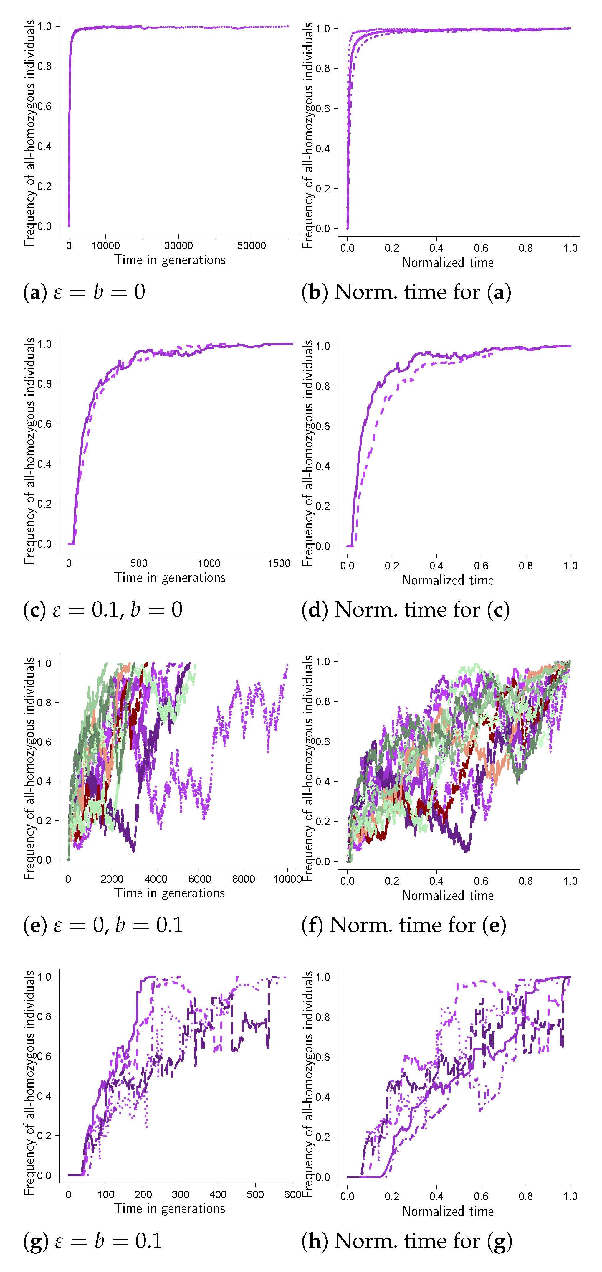
Figure A5.
Three sites with weight function as in Equation (A5). Examples of fixation trajectories at three sites with weight function as in Equation (A5), carrying capacity , cutoff , probability of recombination between adjacent sites, , , (see Equation (7)) and probability of a bottleneck b as shown, strength of selection and bottleneck ; excursions’ trajectories from ten trials in (a,c) and from trials in (e,g). Each trajectory traces, as a function of time, the number of diploid individuals homozygous for the fit type at all sites relative to the population size (the number of diploid individuals). The panels on the right (b,d,f,h) show the corresponding excursions from the left panels (a,c,e,g), where the time to fixation for each excursion is normalized by the time to fixation for the excursion. The scale of the abscissa (time axis) may vary between panels; in each panel, the trajectories were all obtained under identical conditions.

Figure A6.
Three sites with weight function as in Equation (A3). Examples of fixation trajectories for fixation at three sites with weight function given by Equation (A3), carrying capacity , cutoff , probability of recombination between adjacent sites, , , (see Equation (7)) and probability of a bottleneck b as shown, strength of selection and bottleneck ; (a,c) from ten experiments, (e,g) from experiments. Each trajectory traces, as a function of time, the number of diploid individuals homozygous for the fit type at all sites relative to the population size (the number of diploid individuals). The panels on the right (b,d,f,h) show the corresponding excursions from the left panels (a,c,e,g), where the time to fixation for each excursion is normalized by the time to fixation for the excursion. The scale of the abscissa (time axis) may vary between panels; in each panel, the trajectories were all obtained under identical conditions.

Figure A7.
Three sites with weight function as in Equation (A4). Examples of fixation trajectories for fixation at three sites with weight function as in Equation (A4), carrying capacity , cutoff , probability of recombination between adjacent sites, , , (see Equation (7)) and probability of a bottleneck b as shown, strength of selection and bottleneck . In (a,c,e) trajectories from ten experiments, in (g) from experiments. Each trajectory traces, as a function of time, the number of diploid individuals homozygous for the fit type at all sites relative to the population size (the number of diploid individuals). The panels on the right (b,d,f,h) show the corresponding excursions from the left panels (a,c,e,g), where the time to fixation for each excursion is normalized by the time to fixation for the excursion. The scale of the abscissa (time axis) may vary between panels; in each panel, the trajectories were all obtained under identical conditions.

Figure A8.
Three sites with weight function as in Equation (A4). Examples of fixation trajectories at three sites with weight function as given by Equation (A4); carrying capacity , cutoff , probability of recombination between adjacent sites, , , (see Equation (7)) and probability of a bottleneck b as shown, strength of selection and bottleneck . In (a,c), trajectories are from ten experiments; trajectories in (e,g) are from experiments. Each trajectory traces, as a function of time, the number of diploid individuals homozygous for the fit type at all sites relative to the population size (the number of diploid individuals). The panels on the right (b,d,f,h) show the corresponding excursions from the left panels (a,c,e,g), where the time to fixation for each excursion is normalized by the time to fixation for the excursion. The scale of the abscissa (time axis) may vary between panels; in each panel, the trajectories were all obtained under identical conditions.

Appendix B
In this section, we give the algorithm for the simulations in the form of a pseudocode. Each and every time, we started with the fit type in one copy at each site, with any given diploid individual initially carrying at most one copy of a fit type. Each and every time, the population size was initially set to the carrying capacity .
- 1.
- Initialize the frequency of the fit type at each site, i.e.,with any diploid individual being heterozygous at most at one site.
- 2.
- While holds, then for generation started with individuals:
- (a)
- Sample a random uniform on to check if a bottleneck occurs;
- (b)
- where b is the probability of a bottleneck and B the number of individuals surviving a bottleneck;
- (c)
- In the case of a bottleneck, the M surviving individuals are sampled uniformly at random without replacement from among the individuals;
- (d)
- The M individuals randomly form pairs that will go on to produce juveniles;
- (e)
- Sample random number of juveniles according to Equation (7) produced independently by randomly formed parent pairs;
- (f)
- Assign types to the juveniles according to Mendel’s laws allowing for recombination between sites (we exclude mutation);
- (g)
- If , for each juvenile independently, sample a random exponential with rate as in Equation (8), compute the th largest exponential , and a juvenile with exponential survives;
- (h)
- If , all the juveniles survive, so that for any .
- 3.
- Record the result of the trajectory; if the event occurred, a fit type was lost, and if occurred, the fit type reached fixation at all sites, with .
The documented CWEB (C++) code is freely available at https://github.com/eldonb/fixation_many_sites (accessed on 13 December 2022).
References
- Eldon, B. Evolutionary Genomics of High Fecundity. Annu. Rev. Genet. 2020, 54, 213–236. [Google Scholar] [CrossRef] [PubMed]
- Hedgecock, D.; Pudovkin, A.I. Sweepstakes reproductive success in highly fecund marine fish and shellfish: A review and commentary. Bull Mar. Sci. 2011, 87, 971–1002. [Google Scholar] [CrossRef]
- Hedgecock, D. Does variance in reproductive success limit effective population sizes of marine organisms? In Proceedings of the Genetics and Evolution of Aquatic Organisms, Bangor, UK, 10–16 September 1992; Beaumont, A., Ed.; Chapman and Hall: London, UK, 1994; pp. 1222–1344. [Google Scholar]
- Flowers, J.M.; Schroeter, S.C.; Burton, R.S. The Recruitment Sweepstakes Has Many Winners: Genetic Evidence from the Sea Urchin Strongylocentrotus Purpuratus. Evolution 2002, 56, 1445–1453. [Google Scholar] [CrossRef] [PubMed]
- Árnason, E.; Koskela, J.; Halldórsdóttir, K.; Eldon, B. Sweepstakes Reproductive Success Via Pervasive and Recurrent Selective Sweeps. eLife 2023. [Google Scholar] [CrossRef]
- Williams, G. Sex and Evolution; Monographs in Population Biology; Princeton University Press: Princeton, NJ, USA, 1975. [Google Scholar]
- Möhle, M.; Sagitov, S. Coalescent patterns in diploid exchangeable population models. J. Math. Biol. 2003, 47, 337–352. [Google Scholar] [CrossRef]
- Sagitov, S. Convergence to the coalescent with simultaneous mergers. J. Appl. Probab. 2003, 40, 839–854. [Google Scholar] [CrossRef] [Green Version]
- Möhle, M.; Sagitov, S. A classification of coalescent processes for haploid exchangeable population models. Ann. Probab. 2001, 29, 1547–1562. [Google Scholar] [CrossRef]
- Schweinsberg, J. Coalescent processes obtained from supercritical Galton-Watson processes. Stoch. Proc. Appl. 2003, 106, 107–139. [Google Scholar] [CrossRef] [Green Version]
- Eldon, B.; Wakeley, J. Coalescent processes when the distribution of offspring number among individuals is highly skewed. Genetics 2006, 172, 2621–2633. [Google Scholar] [CrossRef] [Green Version]
- Sargsyan, O.; Wakeley, J. A coalescent process with simultaneous multiple mergers for approximating the gene genealogies of many marine organisms. Theor. Pop. Biol. 2008, 74, 104–114. [Google Scholar] [CrossRef]
- Birkner, M.; Blath, J.; Eldon, B. An ancestral recombination graph for diploid populations with skewed offspring distribution. Genetics 2013, 193, 255–290. [Google Scholar] [CrossRef] [Green Version]
- Durrett, R.; Schweinsberg, J. A coalescent model for the effect of advantageous mutations on the genealogy of a population. Stoch. Process. Their Appl. 2005, 115, 1628–1657. [Google Scholar] [CrossRef] [Green Version]
- Birkner, M.; Liu, H.; Sturm, A. Coalescent results for diploid exchangeable population models. Electron. J. Probab. 2018, 23, 1–44. [Google Scholar] [CrossRef]
- Koskela, J.; Berenguer, M.W. Robust model selection between population growth and multiple merger coalescents. Math. Biosci. 2019, 311, 1–12. [Google Scholar] [CrossRef] [Green Version]
- Eldon, B. Genome-wide fixation under viability selection. biorXiv 2022. preprint. [Google Scholar] [CrossRef]
- Eldon, B.; Stephan, W. Sweepstakes reproduction facilitates rapid adaptation in highly fecund populations. Authorea 2022. [Google Scholar] [CrossRef]
- Pitman, J. Coalescents with multiple collisions. Ann. Probab. 1999, 27, 1870–1902. [Google Scholar] [CrossRef]
- Sagitov, S. The general coalescent with asynchronous mergers of ancestral lines. J. Appl. Probab. 1999, 36, 1116–1125. [Google Scholar] [CrossRef]
- Donnelly, P.; Kurtz, T.G. Particle Representations for Measure-Valued Population Models. Ann. Probab. 1999, 27, 166–205. [Google Scholar] [CrossRef]
- Schweinsberg, J. Coalescents with simultaneous multiple collisions. Electron. J. Probab. 2000, 5, 1–50. [Google Scholar] [CrossRef]
- Slade, P. Linearization of the Kingman Coalescent. Mathematics 2018, 6, 82. [Google Scholar] [CrossRef] [Green Version]
- Birkner, M.; Blath, J.; Möhle, M.; Steinrücken, M.; Tams, J. A modified lookdown construction for the Xi-Fleming-Viot process with mutation and populations with recurrent bottlenecks. ALEA Lat. Am. J. Probab. Math. Stat. 2009, 6, 25–61. [Google Scholar]
- Freund, F.; Kerdoncuff, E.; Matuszewski, S.; Lapierre, M.; Hildebrandt, M.; Jensen, J.D.; Ferretti, L.; Lambert, A.; Sackton, T.B.; Achaz, G. Interpreting the pervasive observation of U-shaped Site Frequency Spectra. biorXiv 2022. preprint. [Google Scholar] [CrossRef]
- Birkner, M.; Blath, J. Measure-valued diffusions, general coalescents and population genetic inference. In Trends in Stochastic Analysis; Blath, J., Mörters, P., Scheutzow, M., Eds.; Cambridge University Press: Cambridge, UK, 2009; pp. 329–363. [Google Scholar]
- Der, R.; Epstein, C.L.; Plotkin, J.B. Generalized population models and the nature of genetic drift. Theor. Popul. Biol. 2011, 80, 80–99. [Google Scholar] [CrossRef] [PubMed]
- Dynkin, E. Markov Processes; Springer: Berlin/Heidelberg, Germany, 1965. [Google Scholar]
- Etheridge, A.M.; Griffiths, R.C.; Taylor, J.E. A coalescent dual process in a Moran model with genic selection, and the Lambda coalescent limit. Theor. Popul. Biol. 2010, 78, 77–92. [Google Scholar] [CrossRef]
- Foucart, C. The impact of selection in the Λ-Wright-Fisher model. Electron. Commun. Probab. 2013, 18, 1–10. [Google Scholar] [CrossRef]
- Bah, B.; Pardoux, E. The Λ-lookdown model with selection. Stoch. Process. Their Appl. 2015, 125, 1089–1126. [Google Scholar] [CrossRef]
- Der, R.; Plotkin, J.B. The Equilibrium Allele Frequency Distribution for a Population with Reproductive Skew. Genetics 2014, 196, 1199–1216. [Google Scholar] [CrossRef] [Green Version]
- Greven, A.; Pfaffelhuber, P.; Pokalyuk, C.; Wakolbinger, A. The fixation time of a strongly beneficial allele in a structured population. Electron. J. Probab. 2016, 21, 1–42. [Google Scholar] [CrossRef]
- Orr, H.A. The distribution of fitness effects among beneficial mutations. Genetics 2003, 163, 1519–1526. [Google Scholar] [CrossRef]
- Orr, H.A. The population genetics of beneficial mutations. Philos. Trans. R. Soc. B Biol. Sci. 2010, 365, 1195–1201. [Google Scholar] [CrossRef]
- Bell, G. Fluctuating selection: The perpetual renewal of adaptation in variable environments. Philos. Trans. R. Soc. B Biol. Sci. 2010, 365, 87–97. [Google Scholar] [CrossRef] [Green Version]
- Huillet, T.; Möhle, M. On the extended Moran model and its relation to coalescents with multiple collisions. Theor. Popul. Biol. 2013, 87, 5–14. [Google Scholar] [CrossRef] [Green Version]
- De Vladar, H.P.; Barton, N. Stability and response of polygenic traits to stabilizing selection and mutation. Genetics 2014, 197, 749–767. [Google Scholar] [CrossRef] [Green Version]
- Patwa, Z.; Wahl, L.M. The fixation probability of beneficial mutations. J. R. Soc. Interface 2008, 5, 1279–1289. [Google Scholar] [CrossRef] [Green Version]
- Charlesworth, B. How Long Does It Take to Fix a Favorable Mutation, and Why Should We Care? Am. Nat. 2020, 195, 753–771. [Google Scholar] [CrossRef]
- Barton, N.H. The effect of hitch-hiking on neutral genealogies. Genet. Res. 1998, 72, 123–133. [Google Scholar] [CrossRef]
- Van Herwaarden, O.A.; van der Wal, N.J. Extinction Time and Age of an Allele in a Large Finite Population. Theor. Popul. Biol. 2002, 61, 311–318. [Google Scholar] [CrossRef]
- Kaplan, N.L.; Hudson, R.R.; Langley, C.H. The “hitchhiking effect” revisited. Genetics 1989, 123, 887–899. [Google Scholar] [CrossRef]
- Durrett, R.; Schweinsberg, J. Approximating selective sweeps. Theor. Popul. Biol. 2004, 66, 129–138. [Google Scholar] [CrossRef]
- Kingman, J. The representation of partition structures. J. Lond. Math. Soc. 1978, 18, 374–380. [Google Scholar] [CrossRef]
- Eldon, B.; Stephan, W. Evolution of highly fecund haploid populations. Theor. Popul. Biol. 2018, 119, 48–56. [Google Scholar] [CrossRef] [PubMed]
- Pritchard, J.K.; Pickrell, J.K.; Coop, G. The genetics of human adaptation: Hard sweeps, soft sweeps, and polygenic adaptation. Curr. Biol. 2010, 20, R208–R215. [Google Scholar] [CrossRef] [PubMed] [Green Version]
- Pritchard, J.K.; Di Rienzo, A. Adaptation—Not by sweeps alone. Nat. Rev. Genet. 2010, 11, 665–667. [Google Scholar] [CrossRef] [Green Version]
- Hansen, T.F. WHY epistasis is important for selection and adaptation. Evolution 2013, 67, 3501–3511. [Google Scholar] [CrossRef]
- Malmberg, R.L.; Mauricio, R. QTL-based evidence for the role of epistasis in evolution. Genet. Res. 2005, 86, 89–95. [Google Scholar] [CrossRef]
- Bank, C. Epistasis and Adaptation on Fitness Landscapes. Annu. Rev. Ecol. Evol. Syst. 2022, 53, 457–479. [Google Scholar] [CrossRef]
- Walsh, B.; Blows, M.W. Abundant genetic variation + strong selection = multivariate genetic constraints: A geometric view of adaptation. Annu. Rev. Ecol. Evol. Syst. 2009, 40, 41–59. [Google Scholar] [CrossRef] [Green Version]
- Reznick, D.N. The Origin Then and Now; Princeton University Press: Princeton, NJ, USA, 2011. [Google Scholar]
- Vignieri, S.N.; Larson, J.G.; Hoekstra, H.E. The selective advantage of crypsis in mice. Evol. Int. J. Org. Evol. 2010, 64, 2153–2158. [Google Scholar] [CrossRef]
- Cook, L.M.; Grant, B.S.; Saccheri, I.J.; Mallet, J. Selective bird predation on the peppered moth: The last experiment of Michael Majerus. Biol. Lett. 2012, 8, 609–612. [Google Scholar] [CrossRef]
- Daborn, P.; Yen, J.; Bogwitz, M.; Le Goff, G.; Feil, E.; Jeffers, S.; Tijet, N.; Perry, T.; Heckel, D.; Batterham, P.; et al. A single P450 allele associated with insecticide resistance in Drosophila. Science 2002, 297, 2253–2256. [Google Scholar] [CrossRef]
- Grant, P.R.; Grant, B.R. How and Why Species Multiply; Princeton University Press: Princeton, NJ, USA, 2020. [Google Scholar]
- Losos, J. Lizards in an Evolutionary Tree; University of California Press: Berkely, CA, USA, 2009. [Google Scholar]
- Roemhild, R.; Schulenburg, H. Evolutionary ecology meets the antibiotic crisis: Can we control pathogen adaptation through sequential therapy? Evol. Med. Public Health 2019, 2019, 37–45. [Google Scholar] [CrossRef]
- Lehtinen, S.; Blanquart, F.; Lipsitch, M.; Fraser, C. On the evolutionary ecology of multidrug resistance in bacteria. PLoS Pathog. 2019, 15, e1007763. [Google Scholar] [CrossRef] [Green Version]
- Hawkins, N.J.; Bass, C.; Dixon, A.; Neve, P. The evolutionary origins of pesticide resistance. Biol. Rev. 2018, 94, 135–155. [Google Scholar] [CrossRef] [Green Version]
- Fan, J.Y.; Hamza, K.; Jagers, P.; Klebaner, F.C. Limit theorems for multi-type general branching processes with population dependence. Adv. Appl. Probab. 2020, 52, 1127–1163. [Google Scholar] [CrossRef]
- Yakovlev, A.Y.; Yanev, N.M. Limiting distributions for multitype branching processes. Stoch. Anal. Appl. 2010, 28, 1040–1060. [Google Scholar] [CrossRef] [Green Version]
- Mode, C. Multitype Branching Processes: Theory and Applications; Modern Analytic and Computational Methods in Science and Mathematics; American Elsevier Publishing Company: New York, NY, USA, 1971. [Google Scholar]
- Athreya, K.B.; Ney, P.E. Branching Processes; Springer: Berlin/Heidelberg, Germany, 1972. [Google Scholar] [CrossRef]
- Kersting, G. A unifying approach to branching processes in a varying environment. J. Appl. Probab. 2020, 57, 196–220. [Google Scholar] [CrossRef]
- Vatutin, V.A.; Dyakonova, E.E. Multitype branching processes in random environment. Russ. Math. Surv. 2021, 76, 1019–1063. [Google Scholar] [CrossRef]
- Haldane, J.B.S. The cost of natural selection. J. Genet. 1957, 55, 511–524. [Google Scholar] [CrossRef]
Figure 1.
Fixation at two sites with weight function as in Equation (9). Examples of excursion to fixation at two sites with weight as given by Equation (8) with weight function as given by Equation (9) for carrying capacity , cutoff (see Equation (5)), probability of recombination between adjacent sites, , , with (see Equation (7)) and b (the probability of a bottleneck in a given generation) as shown, strength of selection , bottleneck throughout, number of replicates except ten for (a). Each trajectory traces, as a function of time, the number of diploid individuals homozygous for the fit type at all sites relative to the population size (the number of diploid individuals). The panels on the right (b,d,f,h) show the corresponding excursions from the left panels (a,c,e,g) where the time to fixation for each excursion is normalized by the time to fixation for the excursion. The scale of the abscissa (time axis) may vary between panels; in each panel, the trajectories were all obtained under identical conditions.


Table 1.
The possible genomic configurations with two sites; for denotes a haplotype with type a at site one and type b at site two; the entries are example values of the weight function in Equation (8).
Table 1.
The possible genomic configurations with two sites; for denotes a haplotype with type a at site one and type b at site two; the entries are example values of the weight function in Equation (8).
| 0 | ||||
| 1 | 0 | 1 | ||
| 0 | 1 | 1 | ||
| 1 | 1 | 2 |
Disclaimer/Publisher’s Note: The statements, opinions and data contained in all publications are solely those of the individual author(s) and contributor(s) and not of MDPI and/or the editor(s). MDPI and/or the editor(s) disclaim responsibility for any injury to people or property resulting from any ideas, methods, instructions or products referred to in the content. |
© 2023 by the author. Licensee MDPI, Basel, Switzerland. This article is an open access article distributed under the terms and conditions of the Creative Commons Attribution (CC BY) license (https://creativecommons.org/licenses/by/4.0/).
Share and Cite
MDPI and ACS Style
Eldon, B. Viability Selection at Linked Sites. Mathematics 2023, 11, 569. https://doi.org/10.3390/math11030569
AMA Style
Eldon B. Viability Selection at Linked Sites. Mathematics. 2023; 11(3):569. https://doi.org/10.3390/math11030569
Chicago/Turabian StyleEldon, Bjarki. 2023. "Viability Selection at Linked Sites" Mathematics 11, no. 3: 569. https://doi.org/10.3390/math11030569
Note that from the first issue of 2016, this journal uses article numbers instead of page numbers. See further details here.