Characterization of Flow under Impervious Dams: Dimensionless Groups and Universal Solutions

Abstract

As far as we know, no dimensionless solutions for infiltrated flow under dams in anisotropic media exist since those that can be found in manuals refer to isotropic soils. The novelty of this work is the presentation of universal solutions in the form of abaci for water flow, average exit gradient, uplift force, and its application point for this type of soil. These solutions are obtained by the application of the discriminated nondimensionalization technique to the governing equations in order to find accurate dimensionless groups that control the results of the problem. In particular, the ratio of permeabilities corrected by a geometrical aspect relationship appears as a governing group, so anisotropy can be considered as input information. In this way, the sought solutions are a function of the emerging groups. Numerical solutions are used to successfully verify the results obtained, which in turn are compared to those of other authors for isotropic scenarios.

1. Introduction

Flow through porous media has been a widely studied issue in geotechnics and hydrogeology for decades, and different books [1,2,3] and papers deserve to be cited as references in relevant aspects of this topic, such as flow in saturated and unsaturated media [4] or liquefaction [5,6,7]. According to Haq et al. [8] and Animasaun et al. [9], fluid flow through porous media, as used in fluid mechanics, refers to how fluids behave while passing through a porous substance such as sponge or wood or when filtering water via sand or another porous material [1,2,3,4,5,6,7]. These problems are macroscopically approached with the constitutive law of Darcy [10,11] since their microscopic mathematical treatment is an unworkable task due to the intricate, complex, and heterogeneous structure of the soil net. This law sets the connection between the mean velocity of the groundwater flow and the gradient of the piezometric potential through the hydraulic conductivity, a parameter that collects information from both the soil (porosity, tortuosity, grain size, connectivity) and fluid (viscosity, specific weight) physical properties [12,13,14].

Assuming the incompressibility of fluid and soil grains, their small velocities (negligible inertial forces), and their anisotropic domains, the substitution of the continuity equation in Darcy’s law gives rise to a Laplace-type expression that is the governing equation of the problem (in terms of the potential variable [15]), whose solution may be derived either analytically or numerically [16,17,18]. However, in civil engineering and particularly in the 2D design of retaining structures (such as gravity dams, cofferdams, and earth dams), one of the most common solutions has the form of flow nets [19]. These are graphical representations that directly show the stream function [20] and potential iso-lines within the seepage scenario. The advantage of these patterns, for whose construction simple rules are needed even in complex geometries with different boundary conditions, is to allow the user a direct and easy interpretation of the solution. Other possible means to study flow through porous media are scale models [21], which have been traditionally used to obtain empirical formulation for retaining structures as well as other hydrogeological problems, such as pumping wells [22]. Nowadays, however, the most popular approach to these problems is numerical simulation with commercial or free software code [23,24].

The aim of this paper is to study the phenomenon of flow through anisotropic porous media under gravity dams with and without a foundation, looking for, particularly, the solution of dimensionless unknowns such as water flow, average exit gradient, and uplift force under the dam base and its application point. While for isotropic soils, dimensionless groups and universal solutions are already known in the scientific literature, the same does not apply to anisotropic soils. For this purpose, a technique that combines dimensional analysis [25,26] and spatial discrimination [27,28,29,30] allows us to reduce the governing equation and geometrical conditions to their dimensionless forms, from which the smallest number of independent dimensionless groups that govern the problem emerge. Spatial discrimination states that lengths can only be considered as the same dimension if they are measured in the same direction, so a ratio of a vertical and a horizontal parameter or variable is not dimensionless. Universal solutions are based on the Pi theorem [31], which states that any dimensionless unknown of the problem is an arbitrary function of the correctly deduced dimensionless groups. This technique has already been successfully employed in different engineering problems such as soil consolidation [32,33], solute and heat transport [34], and thermal interference in experimental measurements due to overheating [35].

In previous works [36], several authors presented universal equations or graphics in order to solve the flow of groundwater under dams in 2D isotropic domains. For this purpose, they attempted to find dimensionless groups (such as the ratio between the width of the dam and the thickness of the stratum) that seemed to work correctly. In effect, this is true thanks to the isotropic character of the porous media. Nevertheless, in anisotropic domains, such quotients as well as the ratio of anisotropic hydraulic conductivities ($k_x/k_y$) do not work as independent dimensionless groups. In these anisotropic media, on the one hand, aspect ratios must be quotients that relate lengths of the same spatial direction (as spatial discrimination requires), and on the other hand, as it is deduced from dimensionless governing equations, the ratio of conductivities ($k_x/k_y$) must be accompanied by a certain aspect ratio to define the correct dimensionless groups.

The importance of working on anisotropic soils has been pointed out by many authors for a long time [37,38,39]. Real soils, generally consolidated, can present horizontal hydraulic conductivities with higher values than vertical conductivities depending on the nature of the soil and the depth from where the sample is taken [40]. This fact has an enormous impact on calculations related to soil engineering and, in particular, with the patterns derived from seepage flow.

This document is organized as follows. In the “Mathematical Model” section, the mathematical model of the flow through porous media under gravity dams is briefly presented. The “Discriminated Governing Equations and Dimensionless Groups” section explains the discriminated dimensional characterization method and the dimensionless groups deduced in anisotropic media. The “Verification of the Emergent Discriminated Dimensionless Groups” section verifies the correct characterization of the problem using the deduced dimensionless groups with an example. The “Solutions” section is a compilation of universal abaci obtained by numerical simulation for the following dimensionless variables: water flow, average exit gradient, uplift force, and center of application. For isotropic cases, comparisons with the results of other authors are presented. Finally, a case study is presented, and the contributions and conclusions are summarized.

2. Mathematical Model

The governing equation is an expression obtained by combining the momentum and continuity Equations (1) and (2), respectively. For homogeneous soils and fluids, Darcy’s law, which relates the velocity of the groundwater flow to the change in the potential head, is equivalent to the momentum equation when the problem is studied in macroscopic level, and Equation (1) shows its expression for 2D rectangular media. The continuity equation employed in this study assumes a steady-state scenario with no sources or sinks.

$$\mathit{v}=-k\mathbf{\nabla }h\hspace{1em}\mathrm{or}\hspace{1em}{v}_x=-k_x\frac{\partial h}{\partial x}\hspace{1em}\mathrm{and}\hspace{1em}{v}_y=-k_y\frac{\partial h}{\partial y}$$

(1)

$$\mathbf{\nabla }\times \mathit{v}=0\hspace{1em}\mathrm{or}\hspace{1em}\frac{\partial v_x}{\partial x}+\frac{\partial v_y}{\partial y}=0$$

(2)

Introducing Darcy’s law in Equation (2), the governing equation, a Laplace-type expression, for anisotropic soils in terms of the water potential is obtained, as shown in Equation (3).

$$k_x\frac{{\partial }^{2}h}{\partial x^2}+k_y\frac{{\partial }^{2}h}{\partial y^2}=0$$

(3)

For an isotropic soil, $k_x=k_y=k$, and Equation (3) is simplified to $\frac{{\partial }^{2}h}{\partial x^2}+\frac{{\partial }^{2}h}{\partial y^2}=0$.

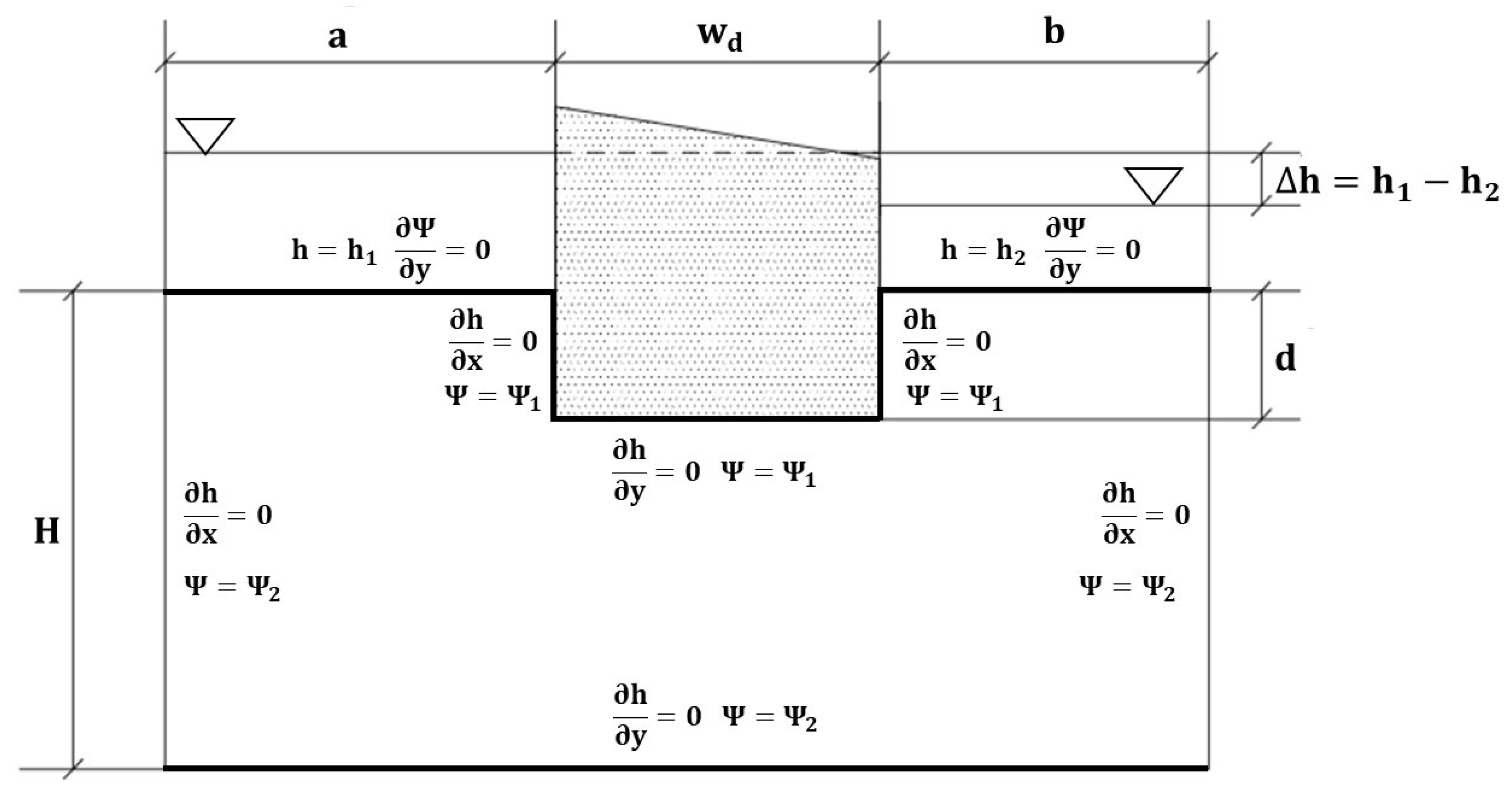
In order to complete the mathematical model, the boundary conditions must be added. For this kind of scenario, only first- and second-class boundary conditions are applied. The first, also called the Dirichlet condition, shown in Equation (4), means that a constant value of water potential is set at the boundary. This boundary condition is applied on the horizontal upstream and downstream length, with values of h₁ and h₂, respectively. These constant water potential values are the reason why the flow is generated since h₁ > h₂. The second-class boundary condition, or Neumann condition, corresponds to impervious borders of the scenario as given in Equation (5). This class is set in all the other borders of the scenario, that is, those in which the dam and the soil are in contact, and the vertical and bottom horizontal borders of the stratum. In this way, the only borders through which water enters and leaves the scenario are the upper horizontal ones, while the others isolate the problem from the rest of the system, so they can be studied independently.

As many problems of flow under retaining structures present several first-class boundary conditions, the analytical resolution of the problem becomes very cumbersome. These equations are written as follows:

$$h=h_{o,r}\hspace{1em}\mathrm{at} \mathrm{boundary} \mathrm{regions} 1,2\dots \mathrm{r}\hspace{1em}\left(\mathrm{first}\mathrm{class}\right)$$

(4)

$${\left.\frac{\partial v}{\partial n}\right|}_s=0\hspace{1em}\mathrm{at} \mathrm{boundary} \mathrm{regions} 1,2\dots \mathrm{s}\hspace{1em}\left(\mathrm{second}\mathrm{class}\right)$$

(5)

with $n$ as the direction normal to the impermeable boundary surface.

Another way to study the flow through porous media is to employ the stream function $\Psi$, which is related to velocity and water head, according to Equation (6). This is a scalar function whose derivative with respect to any direction would lead to the velocity component orthogonal to that direction. If the problem is studied in a graphical way, those points with the same value of stream function generate stream lines.

$$v_x=\frac{\partial \Psi }{\partial y}=-k_x\frac{\partial h}{\partial x},v_y=-\frac{\partial \Psi }{\partial x}=-k_y\frac{\partial h}{\partial y}$$

(6)

Therefore, the Laplace equation for anisotropic soils can also be expressed as a function of this variable, shown in Equation (7), since $\frac{{\partial }^{2}h}{\partial x\partial y}=\frac{{\partial }^{2}h}{\partial y\partial x}$.

$$\frac{1}{k_y}\frac{{\partial }^2\Psi }{\partial x^2}+\frac{1}{k_x}\frac{{\partial }^2\Psi }{\partial y^2}=0$$

(7)

If isotropic soils are modelled, Equation (7) is transformed into equation $\frac{{\partial }^2\Psi }{\partial x^2}+\frac{{\partial }^2\Psi }{\partial y^2}=0$.

Boundary conditions must then be translated to this variable although now first- and second-class conditions have a different meaning. Dirichlet conditions, shown in Equation (8), mean a constant value of flow along a given border, which in this scenario is a way to impose that the contact between the dam and the soil is a stream line, and therefore, no flow can occur through these borders, and the same happens to the vertical and bottom horizontal borders. The value of the stream function along the dam–soil contact, Ψ₁, takes the highest value considered in the problem (which can be water flow value or simply 1), while that along the vertical and bottom horizontal borders, Ψ₂, is commonly 0. In this way, stream line values vary between water flow and 0 or between 1 and 0, but in any case, the highest values are close to the retaining structure, and they are reduced as they grow further. Neumann conditions, shown in Equation (9), are set in those borders where no variation of flow occurs, which for this problem are the upstream and downstream horizontal borders. This means that water flows through these borders from upstream to downstream, allowing it to enter and leave the system.

$$\Psi ={\Psi }_{o,p}\hspace{1em}\mathrm{at} \mathrm{boundary} \mathrm{regions} 1,2\dots \mathrm{p}\hspace{1em}\left(\mathrm{first}\mathrm{class}\right)$$

(8)

$${\left.\frac{\partial \Psi }{\partial n}\right|}_q=0\hspace{1em}\mathrm{at} \mathrm{boundary} \mathrm{regions} 1,2\dots \mathrm{q}\hspace{1em}\left(\mathrm{second}\mathrm{class}\right)$$

(9)

Figure 1 presents the geometry and boundary conditions in terms of water potential and stream function variable.

Note that if Equation (7) is multiplied by the factor $k_x·k_y$, Equation (10) is obtained, which is similar to Equation (3) and represents the same phenomenon although employing different variables.

$$k_x\frac{{\partial }^2\Psi }{\partial x^2}+k_y\frac{{\partial }^2\Psi }{\partial y^2}=0$$

(10)

In fact, in 2D scenarios such as the one presented in this paper, water potential and stream function are orthogonal, and so are Equations (3) and (7). For this reason, stream function values can be obtained by numerical integration employing Equation (6) with the proper values of water potential and a constant of integration for the stream function variable [41]. In addition, boundary conditions presented in Equations (8) and (9) in terms of stream function variable are related to those of Equations (3) and (4) in terms of water potential, as they are translated as the impervious boundary along the dam–soil contact, vertical and bottom horizontal borders (Equations (5) and (8)), and borders through which flow can occur applied to the upstream and downstream horizontal borders (Equations (4) and (9)).

Although the problem can be addressed employing either the water potential or the stream function variable, in the following sections, the discriminated dimensionless groups are obtained employing the first since finding the dimensionless form of the unknown expression is easier if the water potential variable is used.

3. Discriminated Governing Equations and Dimensionless Groups

The discriminated nondimensionalization technique is a way to study seepage scenarios in a summarized way. This states that any dimensionless unknown of the problem can be expressed as a function of the dimensionless groups involving both geometrical and hydrogeological variables. Although dimensionless numbers or groups have been traditionally employed in several study fields, the discriminated approach is relatively new. As is known, the derivation of the dimensionless groups in a given problem allows the solutions to be only dependent on such groups instead of each of the physical and geometric parameters involved (as Pi theorem sets). Nevertheless, the way in which dimensionless numbers are derived is not unique. The most general procedure uses concepts of classical dimensional analysis, frequently leading to scarcely precise groups that, however, are very extended in engineering (for example, the Reynolds number in fluid mechanics [42] or flow through a porous medium [43]). Nonetheless, this classical technique cannot be applied in scenarios with anisotropic soils. The principle of discriminated nondimensionalization is precisely solving anisotropic problems, generating completely dimensionless groups that can be used in these scenarios since the technique enforces the groups be rigorously dimensionless both in the units and in the spatial directions of the variables involved. When introducing the concept of spatial discrimination, the smallest number of groups governing the problem is obtained, and some of the classical numbers, such as Reynolds, Rayleigh, and others, emerge with new definitions in terms of the physical and geometrical parameters involved in the problem. To apply this technique, the following steps must be followed:

(i) References to transform the dimensional variables and unknowns in their dimensionless form must be chosen, so the values they take are generally within the interval (0, 1). In this step, any vector variable, such as length or velocity, turns into a dimensionless variable according to its direction;

(ii) The new dimensionless variables are introduced in the governing equations, so each of their addends can be split into two factors. The first is dimensionless and is formed by the new variables and their derivatives, while the second, which is dimensional, clusters the physical and geometrical parameters;

(iii) Since the dimensionless factors are supposed to be of the order of magnitude of the unit, and the governing equation must be balanced, the dimensional factors must have the same order of magnitude;

(iv) The independent ratios formed by pairs of dimensional factors are the discriminated dimensionless groups that govern the problem. The maximum number of dimensionless groups is the number of dimensional factors minus one. According to Pi theorem, the dimensionless solutions or patterns of the study problem are then a function of these discriminated groups [31].

The selected references for variables $x$, $y$, and $h$ are $w_d$, $H$, and $\Delta h$, respectively. Hence, the dimensionless variables are as follows:

$$x^{\prime }=\frac{x}{w_d}\hspace{1em}{y}^{\prime }=\frac{y}{H}\hspace{1em}{h}^{\prime }=\frac{h}{\Delta h}$$

(11)

Introducing these in Equation (3) yields the following:

$$k_x\frac{\Delta h}{w_d{}^2}\frac{{\partial }^2{h}^{\prime }}{\partial {x^{\prime }}^2}+k_y\frac{\Delta h}{H^2}\frac{{\partial }^2{h}^{\prime }}{\partial {y^{\prime }}^2}=0$$

(12)

According to this equation, the solution does not depend on the change of the water potential upstream and downstream the dam. Now, assuming that the derivative factors $\frac{{\partial }^2{h}^{\prime }}{\partial {x^{\prime }}^2}$ and $\frac{{\partial }^2{h}^{\prime }}{\partial {y^{\prime }}^2}$ are of an order of magnitude unit due to the ranges chosen for the dimensionless variables $h^{\prime }$, $x^{\prime }$, and $y^{\prime }$, the only dimensionless group that can be obtained from the former equation is as given below:

$${\pi }_1=\frac{k_x{H}^2}{k_y{w}_d{}^2}$$

(13)

A more thorough discussion of how group ${\pi }_1$ is deduced can be found in Alhama et al [44].

Group ${\pi }_1$ can also be obtained if instead of the water potential variable, the stream function variable is turned into dimensionless and introduced in Equation (10).

$$x^{\prime }=\frac{x}{w_d}\hspace{1em}{y}^{\prime }=\frac{y}{H}\hspace{1em}{\Psi }^{\prime }=\frac{\Psi }{\Delta \Psi }$$

(14)

$$k_x\frac{\Delta \Psi }{w_d{}^2}\frac{{\partial }^2{\Psi }^{\prime }}{\partial {x^{\prime }}^2}+k_y\frac{\Delta \Psi }{H^2}\frac{{\partial }^2{\Psi }^{\prime }}{\partial {y^{\prime }}^2}=0$$

(15)

As happened when the potential variable was used, the solution does not depend on the change of stream function, and making the same assumptions, the monomial ${\pi }_1$ can be deduced.

Moreover, other groups appear when studying the scenario from a geometrical point of view. These new groups, Equations (16)–(18), are related to the geometrical conditions, so they are not necessarily of an order of magnitude unit.

$${\pi }_2=\frac{d}{H}$$

(16)

$${\pi }_3=\frac{a}{w_d}$$

(17)

$${\pi }_4=\frac{a}{b}$$

(18)

where ${\pi }_1$ is a kind of permeability ratio corrected by a convenient aspect factor (a clearly new group coming from the discrimination technique); ${\pi }_2$ and ${\pi }_3$ characterize vertical and horizontal flow, respectively, due to the geometric lengths that set the problem (a result also derived from discrimination); and ${\pi }_4$ presents additional information of the scenario in the horizontal direction (in this case, it reflects the asymmetry).

The choice of criteria to define the groups ${\pi }_2$ to ${\pi }_4$ is arbitrary (other length ratios could have been chosen) although the discrimination has to be satisfied; that is, the lengths that define each group must have the same spatial direction. Furthermore, the combination of any of the groups ${\pi }_3$ and ${\pi }_4$ with ${\pi }_1$ also enables redefining ${\pi }_1$. Thus, the choice of the set of (four) independent groups for this problem is left to the experienced researcher and is generally related to the numerical values adopted by the parameters from the real scenarios and the influence of these parameters on the solution of the problem.

Unknown variables must also be transformed into their dimensionless form, and for this purpose, reference values are needed. The first variable to be changed is the groundwater flow, for which the reference value is deduced as follows. Writing the average horizontal flow as $Q_{ref}=v_x{S}_x$, where $v_x$ is the horizontal velocity, and $S_x$ is the cross-section under the dam, and substituting $v_x$ from Darcy’s law, i.e., $v_x=-k_x\frac{\partial h}{\partial x}$, and $S_x=L_y{L}_z$, this reference flow becomes $Q_{ref}=-k_x\frac{\partial h}{\partial x}{L}_y{L}_z$. Now, the variables involved in this formulation can be replaced by parameters of the studied scenario. That is, $Q_{ref}=-k_x\frac{\Delta h}{w_d}H$ since a 2D problem is studied, and $L_z$ = 1. According to Equation (13), $\frac{H}{w_d}~\sqrt{\frac{k_y}{k_x}}$, so $Q_{ref}$ can be modified, leading to the following:

$$Q_{ref}=\sqrt{k_x{k}_y}\Delta h$$

(19)

which is an expression that is commonly employed by several authors [37,38] when anisotropic soils are considered but without any expressed justification. The value of the dimensionless water flow group takes the form below:

$${\pi }_Q=\frac{Q}{\sqrt{k_x{k}_y}\Delta h}$$

(20)

The next unknown variable we are interested in is the uplift force under the dam. This is obtained by integration of the pore pressure right under the retaining structure. If the dam has no foundation, and there is no water potential downstream the dam ($h_2$), the shape of the pore pressure distribution is very similar to a triangle, and it becomes a trapezoid when there is a foundation and/or water potential downstream the retaining structure (Figure 2). Therefore, the uplift force $F$ (area t in Figure 2) can be calculated as an addition of a rectangular area (I), which depends on the position of the foundation ($d$), on the water head value downstream the dam ($h_2$), and a quasi-triangular area (II), which is the part related to the variation of water potential ($\Delta h$). In order to obtain a dimensionless variable between 0 and 1, the rectangular area (I) must be subtracted, and the remaining area (II) is turned into a dimensionless value by applying the theoretical maximum pore pressure area as a reference force. In this way, the expression that provides the dimensionless group of the searched uplift force is given by the following:

$${\pi }_{UF}=\frac{F-w_d{\gamma }_w\left(h_2+d\right)}{w_d{\gamma }_w\Delta h}$$

(21)

The following studied variable is the application point of the uplift force, which is obtained dividing the momentum due to the pore pressure under the dam by the uplift pressure. In this case, it is calculated with respect to the heel of the dam. As occurs for the uplift force, in order to calculate the dimensionless expression of this unknown, the pore pressure distribution is also divided into its rectangle and triangle components (Figure 2). The application point of the uplift pressure due to the rectangular area (I) is always located in the middle of the dam width ($C_i=c_i/w_d=$ 0.5). However, that due to area II varies its position according to the shape and is never lower than $C_i=c_i/w_d=$ 0.33 or higher than 0.5. In this way, the dimensionless expression of the application point is as given below:

$${\pi }_C=\frac{\frac{c}{w_d}F-\left(h_2+d\right)w_d{\gamma }_{w}0.5}{F-\left(h_2+d\right)w_d{\gamma }_w}$$

(22)

The last variable that is presented in this document is the average exit gradient, $I_{e,ave}$, which is of importance when studying dams (or retaining structures in general) from the safety point of view, especially in reference to piping. The exit gradient (I) is calculated as the difference of hydraulic potential between the downstream highest and lowest points of the buried length (the dam foundation in this study) divided by the value of this length. Standards such as Eurocode-7 [45] propose this definition to the variable, and according to them, these potential values are measured in a column of negligible thickness, so the only information that contributes to the calculation is that right next to the retaining structure. Harr [36] presented several graphics and formulations for obtaining the value of the exit gradient at the point right downstream the retaining structure ($i_e$), so again, only the data beside it are involved. Nevertheless, as a way to consider a larger area and carry out more realistic calculations, Harr also came up with an area for obtaining the value of an average exit gradient, $I_{e,ave}$. This area has the vertical length of the buried length and the horizontal length of half of this buried length. Nevertheless, since Harr only considered isotropic soils, this area is not correct for anisotropic scenarios. A new way to obtain this horizontal length is by multiplying Harr’s expression by an anisotropic factor. In this way, in the study presented in this paper, the vertical length, $l_v$, along which the gradient is calculated, is the dam foundation, d, while the horizontal length, $l_h$, is $\frac{l_v}{2}\sqrt{\frac{k_x}{k_y}}$.

The average exit gradient, $I_{e,ave}$, is traditionally considered as a dimensionless variable, as it is the ratio of two lengths: water head variation, which is measured as a length (as a reduction of the units involved in its definition), and the length of the dam foundation. However, if considering spatial discrimination, each variable, although a length, is measured in a different direction: the variation of water potential in meters of water column and the foundation length in meters in the vertical direction. Therefore, the average exit gradient does have units according to spatial discrimination: $\left[I_{e,ave}\right]=\frac{L_{wc}}{L_y}$. $L_{wc}$ is the dimension of the water potential since, although it is measured in meters and can sometimes coincide with a vertical length, it is an energetic term and cannot be considered as a length in any direction. The dimensionless expression of this variable is obtained dividing the average exit gradient by the ratio of the total variation of water potential of the problem ($\Delta h$, measured in $L_{wc}$) and a vertical length of scenario (measured in $L_y$). For this research, the chosen expression to turn the variable into dimensionless is as follows:

$${\pi }_{Ie,ave}=\frac{I_{e,ave}·H}{\Delta h}$$

(23)

The dimensional values of the variables presented in this paper ($Q$, $F$, $c$, and $I_{e,ave}$) can be obtained employing the expressions of the dimensionless variables in this section (${\pi }_Q$, ${\pi }_{UF}$, ${\pi }_C$, and ${\pi }_{Ie,ave}$) and the abaci shown later, and once they are calculated, they can be used to evaluate the safety of the structure. Therefore, the average exit gradient is utilized when studying the risk of piping or heaving downstream the dam, while the pore pressure distribution (or, in a summarized way, the uplift force and its application point) influences the stability of the structure either to sliding or rotation. For any of the verifications, more information of the problem is needed: soil unit weight, dam dimensions, and characteristics of the zone where the structure is built, among other features. In addition, knowing the amount of the groundwater flow is also useful in order to consider all the possible phenomena occurring in the downstream area.

4. Verification of the Emergent Discriminated Dimensionless Groups

In this section,

Table 1. Scenarios for verification of dimensionless groups (h₁ = 10 m, h₂ = 0 m, Δh = 10 m, k_x, and k_y × 10⁻⁴).

Case	a (m)	b (m)	wd (m)	h (m)	d (m)	kx (m/s)	ky (m/s)	π1	π2	π3	π4	πQ	πUF	πC	πIe,ave
1	50	50	10	10	2.5	1.00	1.00	1	0.25	5	1	0.354	0.500	0.406	0.596
2	75	75	15	4.74	1.186	1.00	0.10	1	0.25	5	1	0.353	0.500	0.406	0.596
3	50	50	10	22.36	5.59	1.00	1.00	5	0.25	5	1	0.481	0.500	0.427	0.782
4	100	100	20	31.62	7.906	1.00	0.50	5	0.25	5	1	0.481	0.500	0.427	0.782
5	50	50	10	10	5	1.00	1.00	1	0.50	5	1	0.244	0.500	0.411	0.377
6	75	75	15	4.74	2.37	1.00	0.10	1	0.50	5	1	0.244	0.500	0.411	0.377
7	10	10	10	10	2.5	1.00	1.00	1	0.25	1	1	0.339	0.500	0.409	0.610
8	20	20	20	15	3.75	2.00	1.125	1	0.25	1	1	0.339	0.500	0.409	0.610
9	50	8.33	10	10	2.5	1.00	1.00	1	0.25	5	6	0.341	0.516	0.411	0.656
10	60	10	12	3.975	0.949	1.00	0.10	1	0.25	5	6	0.341	0.516	0.411	0.656

presents the scenarios and results of ten cases that were solved employing numerical simulation. It shows the geometrical and hydrogeological parameters of this set of ten suitable scenarios. The monomials ruling the problem, ${\pi }_1$ to ${\pi }_4$, were calculated with these parameters and are also presented in Table 1. Cases are paired as follows:

• Cases 1 and 2 are assumed as reference, and although they present different values for the parameters describing the scenario, they have the same value for the four monomials, so they are the same base dimensionless scenario where ${\pi }_1$ = 1, ${\pi }_2$ = 0.25, ${\pi }_3$ = 5, and ${\pi }_4$ = 1. This is the reason why they give the same solution pattern (Figure 3a) according to Pi theorem. Note that the geometrical dimensional scale is not written since it depends on the specific case;
• Cases 3 and 4 also present different values for the parameters describing the scenario. The dimensionless monomials governing the problem are ${\pi }_1$ = 5, ${\pi }_2$ = 0.25, ${\pi }_3$= 5, and ${\pi }_4$ = 1; that is, the value of π₁ is higher than in cases 1 and 2, so the magnitude of the horizontal flow is increased;
• Cases 5 and 6 have the following monomials ruling the problem: ${\pi }_1$ = 1, ${\pi }_2$ = 0.5, ${\pi }_3$ = 5, and ${\pi }_4$ = 1, which means that the dam foundation is deeper than in cases 1 and 2;
• Cases 7 and 8 can be summarized with the following monomials: ${\pi }_1$= 1, ${\pi }_2$ = 0.25, ${\pi }_3$ = 1, and ${\pi }_4$ = 1, reducing the horizontal length of the scenario both upstream and downstream;
• Cases 9 and 10 have the following monomials ruling the scenario: ${\pi }_1$ = 1, ${\pi }_2$ = 0.25, ${\pi }_3$ = 5, and ${\pi }_4$= 6, which means a reduction of the horizontal length of the scenario only downstream the dam.

The equipotential and streamline solutions are all represented in Figure 3. and as expected, each pair has the same pattern despite the different values of the parameters between each case. The range of values for the parameters was chosen to be broad enough to clearly warrant different scenarios. Results of dimensionless expressions of water flow, average exit gradient, uplift force, and its application point are also shown in Table 1. Again, as expected, for each of the pairs, the dimensionless unknowns are the same value since the data monomials are not altered.

According to the results presented in Table 1, the emergent discriminated dimensionless groups (and the technique with which they are derived) are validated. The only slightly different values, those of ${\pi }_Q$ for cases 1 and 2, are due to rounding to three significant figures (the expansion to four figures in ${\pi }_Q$ is 0.3536 for case 1 and 0.3533 for case 2).

From the results in Table 1, some conclusions about the relative importance of the discriminated dimensionless groups can be derived. If ${\pi }_1$ varies from 1 (cases 1 and 2) to 5 (cases 3 and 4), keeping the values of the other monomials constant, the dimensionless water flow changes by a high percentage (more than 30%), and the difference between the values of ${\pi }_C$ is also significant (around 5%) in comparison to the other groups of simulations.

Referring to the change in ${\pi }_2$, from 0.25 (cases 1 and 2) to 0.5 (cases 5 and 6), this also influences the water flow, reducing this value by around 30%. The dimensionless application point (${\pi }_C$) also varies although, as for changes of ${\pi }_1$, this variation is lower than that for ${\pi }_Q$ (less than 5%).

The importance of ${\pi }_3$ is not as significant as ${\pi }_1$ and ${\pi }_2$, especially whether it takes values higher than 10, as we see later. From ${\pi }_3$ = 5 (cases 1 and 2) to ${\pi }_3$ = 1 (cases 7 and 8), the scenario decreases the reservoir length, causing a reduction of the amount of water flowing through the porous medium. This decrease, however, is not as important in percentage terms as the increase due to the increment of ${\pi }_1$ or the reduction because of the increment of ${\pi }_2$. In this third case, the decrease is less than 10%. Looking at the dimensionless application point now, this variation is even lower: less than 1%.

The last scenario variation is associated with the symmetry in the geometry of the problem, that is, ${\pi }_4$. Changing this group from 1 (cases 1 and 2) to 6 (cases 9 and 10) means that a scenario that originally presented the same length upstream and downstream the dam now has a downstream length six times smaller. This variation can be relevant or not according to the value of the other groups, especially ${\pi }_3$, for which values close to unity make ${\pi }_4$ significant. However, as ${\pi }_3$ increases, the effect of ${\pi }_4$ becomes less important. In order to prove this effect, cases 9 and 10 present a high value of ${\pi }_4$, namely 6, even higher than ${\pi }_3$. Although the variations of ${\pi }_Q$ and ${\pi }_C$ are quite low, as with the changes of ${\pi }_3$, something unusual appears: for the other validation cases, where the medium is symmetrical, the dimensionless value of the uplift force, ${\pi }_{UF}$, maintained a constant value of 0.5; however, the asymmetrical scenario increases this value to 0.516.

If the average exit gradient is now observed, monomials ${\pi }_1$ and ${\pi }_2$ also seem more relevant than ${\pi }_3$. As occurs for the water flow, an increase of ${\pi }_1$ from 1 to 5 (cases 1 and 2–cases 3 and 4) leads to an increase of the dimensionless average exit gradient (approximately 30%) as well as an increase of ${\pi }_2$ from 0.25 to 0.5 (cases 1 and 2–cases 5 and 6) leading to a decrease of ${\pi }_{Ie,ave}$ (around 35%). Nevertheless, the difference of values due to the change of ${\pi }_3$ from 5 to 1 (cases 1 and 2–cases 7 and 8) is significatively lower (not even 3%). Finally, the effect of increasing the value selected for ${\pi }_4$ from 1 to 6 becomes a little more important, increasing the value of by about 10%.

5. Solutions

5.1. Universal Curves

Once the validity of the discriminated nondimensionalization technique was proven, a large number of simulations were carried out in order to obtain abaci and universal solutions that simplify the study of flow through isotropic and anisotropic media under gravity dams for future research. The problems were simulated employing a free code based on the network method [41] and the electrical analogy, a methodology that has been successfully applied in other fields of engineering and, specifically, in ground engineering, such as soil consolidation [46] or solute and heat transport [34]. Ngspice [47] was the chosen program to simulate the electrical circuits derived from electrical analogy.

The assumptions of the numerical model are the following:

• The stratum is horizontal, as well as the base of the dam, so the geometry of the scenario is simplified;
• The dam is completely impervious, as it is considered of concrete, so no flow can occur through it;
• The horizontal upstream and downstream lengths are considered to have the same value since in most of the practical cases, these two parameters are much larger than the dam width, so the scenario can be considered as symmetric.

The universal curves presented here attempt to cover a large range of theoretical and realistic situations and scenarios. For this, the values of the data dimensionless groups, which are obtained from the geometric and geotechnical parameters of the problem [1,20,36], are the following:

${\pi }_1$ = (0.03, 0.1, 0.3, 0.5, 1, 2, 5, 10, 30);

${\pi }_2$ = 0–0.75 (although the average exit gradient is not measured for ${\pi }_2$ = 0);

${\pi }_3$ = (1, 2, 5, ≥10);

${\pi }_4$ = 1.

The reason why ${\pi }_4$ presents a value of 1 in this document is to simplify the given solutions. Moreover, since in actual scenarios, a and b commonly take large values compared to those of $w_d$, the problem can be considered as symmetrical, as monomial ${\pi }_4$ loses importance in these cases.

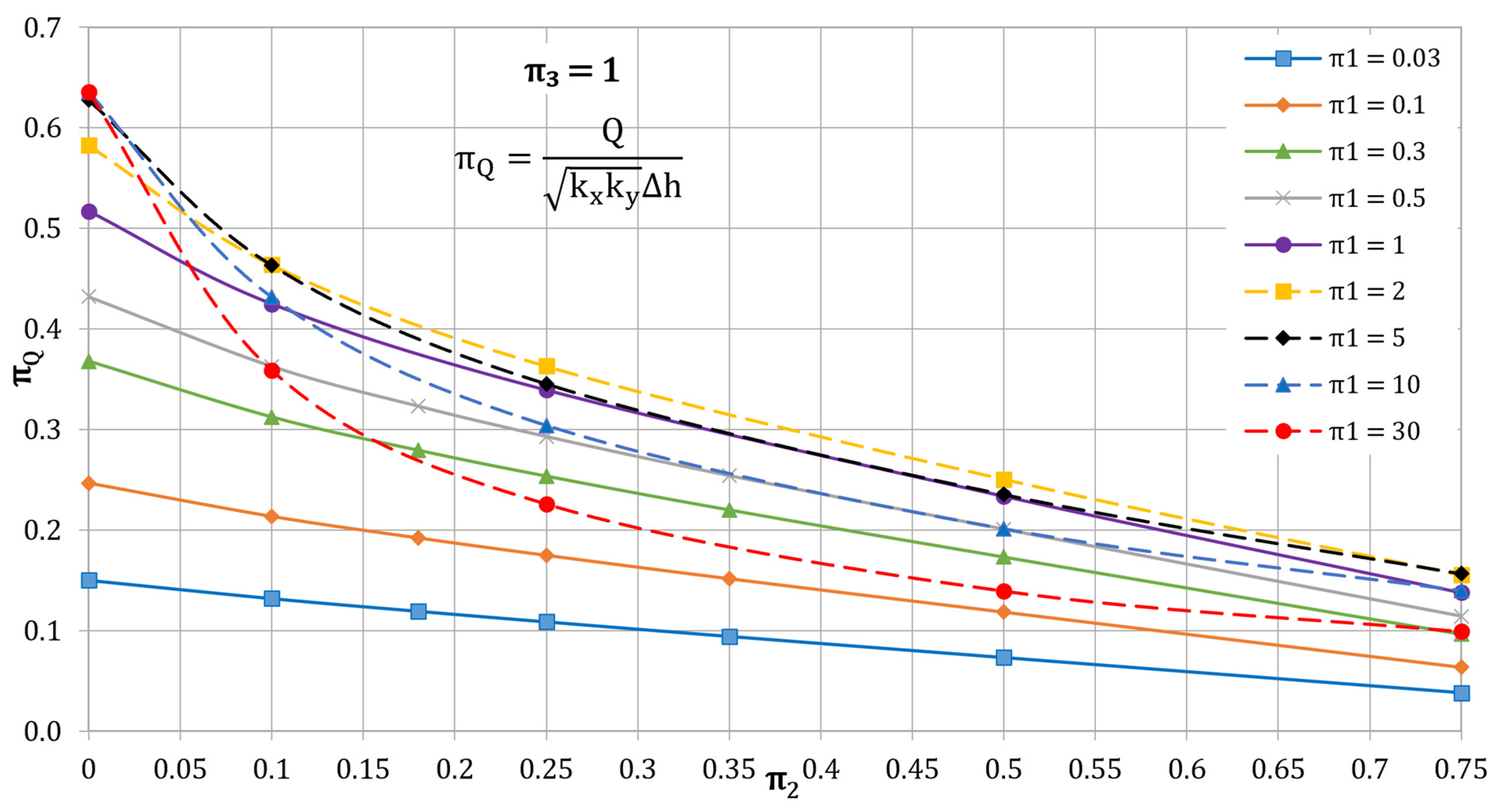
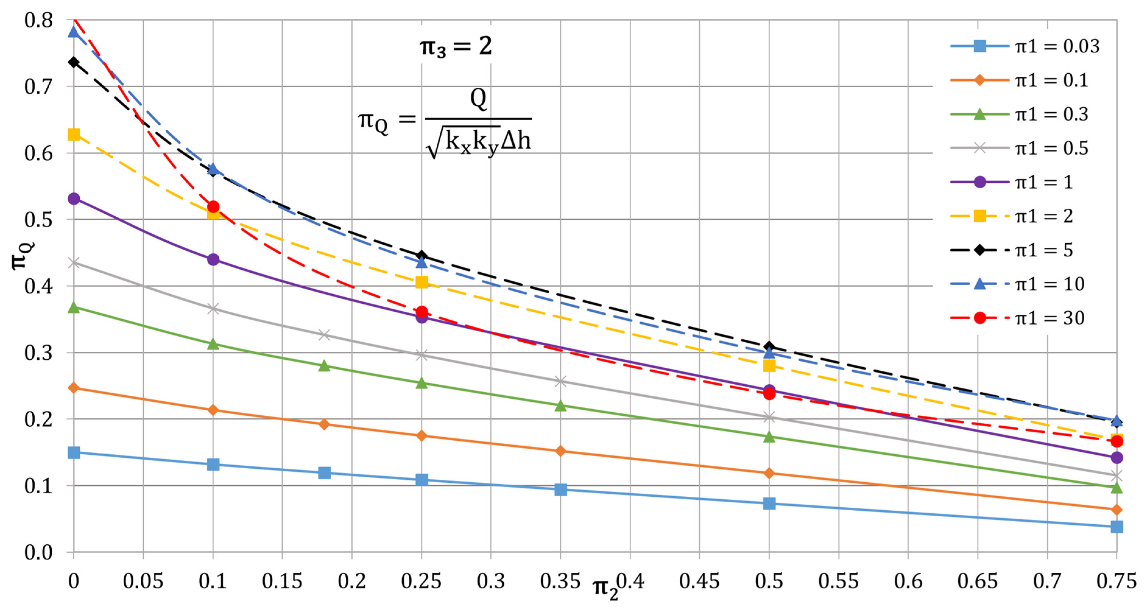
Firstly, the water flow abaci are presented. ${\pi }_2$ is represented in the horizontal axis and the unknown dimensionless variable ${\pi }_Q$ in the vertical axis. Three abaci, one for each value of ${\pi }_3$, are shown (Figure 4, Figure 5 and Figure 6).

According to Figure 4, Figure 5 and Figure 6, the groundwater flow under the retaining structure increases with the value of ${\pi }_1$. This is coherent since this dimensionless group is a comparison of the ease with which the water runs through a porous medium horizontally and vertically. Therefore, as the flow under the gravity dam is essentially horizontal (or at least, that is its nature), the higher ${\pi }_1$, the easier it is for the water to flow through the soil and the higher the total flow obtained. Nevertheless, some exceptions appear for dams with foundation (${\pi }_2$ > 0). When studying ${\pi }_Q$ for high values of ${\pi }_1$ (≥5) but low values of ${\pi }_3$ (1 and 2), the horizontal flow is stimulated and restricted at the same time, respectively. For this reason, in Figure 4, curves for ${\pi }_1$ = 5, 10, and 30 are below those with smaller values, and in Figure 5, the same happens for ${\pi }_1$ = 10 and 30. In Figure 6, where the medium is large enough in the horizontal direction, ${\pi }_1$ affects ${\pi }_Q$ as expected.

In addition, ${\pi }_2$ also seems to be highly decisive for determining the amount of water obtained downstream the dam. The higher the value of this dimensionless group, the deeper the foundation of the dam for the same scenario, leading to an increase in the importance of the vertical flow. For this reason, as the value of ${\pi }_2$ increases, the dimensionless water flow decreases. Finally, the importance of ${\pi }_3$ appears to be reduced as the value of ${\pi }_1$ is decreased, observing that for ${\pi }_1$= 0.03–1, curves of ${\pi }_Q$ are basically the same for all ${\pi }_3$ studied. This effect also occurs for medium-high ${\pi }_1$ (2, 5, and 10) and ${\pi }_3$ (≥5).

When studying the verification results in Table 1, it is seen that for symmetric scenarios where the upstream and downstream horizontal lengths are the same, the dimensionless value ${\pi }_{UF}$ remains constant. Moreover, with the many simulations carried out to develop the abaci for dimensionless groundwater flow and application point of the uplift force, this statement is reaffirmed. Therefore, when studying a symmetrical problem or a problem that can be simplified as symmetrical, the uplift force is as follows:

$${\pi }_{UF}=\frac{F-w_d{\gamma }_w\left(h_2+d\right)}{w_d{\gamma }_w\Delta h}=0.5$$

(24)

The next variable to study is the dimensionless application center, ${\pi }_C$, whose corresponding abaci are shown in Figure 7 and Figure 8.

Paying attention to the effect of ${\pi }_1$ in the value of the application point of the uplift force, the higher the horizontal flow, the bigger the value of ${\pi }_C$. This occurs because the increase in the horizontal flow with respect to the vertical flow means a decrease in the pore pressure in the uplift half of the dam base and an increase of this variable in the downstream half, shifting the application point towards the geometrical center of the dam base.

The effect of the variation of ${\pi }_2$ is also important to observe. If the dimensional position of the application point with respect to the width of the dam is studied, it moves towards the center of the dam as the foundation is deeper. This occurs because the rectangular area of the pore pressure function becomes larger due to the foundation depth. Nevertheless, for (approximately) ${\pi }_2$ > 0.5, the rectangular area continues increasing, whereas the quasi-triangular area hardly varies although the variation of the real application point is not as high as for the previous values of ${\pi }_2$. For this reason, the value of ${\pi }_C$ (which is exclusively associated with the quasi-triangular area) decreases at the end the curve for all values of $\pi$.

The last group to consider, ${\pi }_3$, seems to imply variations in ${\pi }_C$. For those curves of low ${\pi }_1$, ${\pi }_C$ is not affected by ${\pi }_3$. For large values of ${\pi }_1$, as ${\pi }_3$ increases, ${\pi }_C$ decreases, which can be observed in the abaci (Figure 7 and Figure 8).

In this way, the constant value of ${\pi }_{UF}$ is complemented with the ${\pi }_C$ abaci. The shape of the pore pressure distribution is a trapeze, so it can be decomposed in a rectangle, which is basically due to the depth of the foundation, and a quasi-triangle due to the variation of potential along the dam base. As the dimensionless form of the uplift force subtracts the part due to the position of foundation, this is, the rectangular part, the remaining part takes a constant value 0.5 because of the triangular shape. The dimensionless form of the application point of the uplift force is the variable that changes according to the exact shape of the pore pressure distribution when the foundation position part is not considered.

Finally, the last variable to examine is the average exit gradient ${\pi }_{Ie,ave}$, and its abaci are shown in Figure 9 and Figure 10.

The effect of ${\pi }_1$ on this variable is very similar to the effect on ${\pi }_Q$ and ${\pi }_C$; that is, the larger the value of ${\pi }_1$, the larger ${\pi }_{Ie,ave}$ turns out to be. This occurs because, as horizontal flow increases its importance with respect to vertical flow, more change in hydraulic potential occurs on the side of the dam foundation instead of under its base.

When studying how ${\pi }_2$ affects ${\pi }_{Ie,ave}$, this is also quite evident: as the dam foundation becomes deeper, the average gradient decreases. This effect appears because the buried length is increased in a higher proportion than the exit hydraulic potential differences, which leads to a lower value of average exit gradient, and therefore, the dimensionless variable is also lower.

The influence of ${\pi }_3$ is less evident, as it is somehow related to ${\pi }_1$ and ${\pi }_2$, meaning that a concrete effect cannot be found. Figure 9, for which values of ${\pi }_3$ are 1 and 2, shows that for low values of ${\pi }_1$ (<1), values of ${\pi }_{Ie,ave}$ are lower for ${\pi }_3$ = 1 until a certain value of ${\pi }_2$, in which both curves (${\pi }_3$ = 1 and 2) almost join together. ${\pi }_{Ie,ave}$ curves for ${\pi }_1$ = 1 in Figure 9 present a similar behavior although instead of having the same values from a certain value of ${\pi }_2$, the trend is changed, with the values related to ${\pi }_3$ = 1 becoming higher than those of ${\pi }_3$ = 2. For ${\pi }_1$ > 1, values of ${\pi }_{Ie,ave}$ are always lower for curves of ${\pi }_3$ = 2.

Figure 10, which shows the same curves as Figure 9 but for ${\pi }_3$ = 5 and 10, presents a slightly different picture. Low values of ${\pi }_1$ (0.03–0.5) present curves similar to those of Figure 9: the one representing a lower value of ${\pi }_3$ (5 in this case) is below the curve of higher ${\pi }_3$ until a given value of ${\pi }_2$ is reached, and from this, both curves are almost the same. ${\pi }_1$ = 1 curves behave in the same way as in Figure 9 (that is, they change their trend from a certain ${\pi }_2$), and this behavior also appears in curves ${\pi }_1$ = 2–10. Finally, ${\pi }_1$ = 30 curves show similar behavior to that shown in Figure 9, as for all lengths of the dam foundation, ${\pi }_{Ie,ave}$ values are lower for ${\pi }_3$ = 10 than ${\pi }_3$ = 5.

5.2. Comparisons with the Results of Other Authors

Since the universal solutions existing in the literature only refer to the isotropic domain (Muskat [20] for water flow values and Harr [36] for pore pressure under several points of a dam without foundations), comparisons for these results are presented below. The scenario that is compared is a dam with the following geometrical and hydrogeological characteristics:

$a=$100 m;

$b=$ 100 m;

$w_d=$ 10 m;

$d=$ 0 m;

$k_x=k_y=$ 10⁻⁴ m/s;

$H=$ (0.2, 1.25, 2.5, 5, 100) m.

The lowest and highest values of $H$ are only considered for pore pressure verifications since Muskat’s solution only reaches a ratio of $w_d/H$ of 10 and does not report valuable information for $w_d/H$ = 0.1.

Table 2. Verification of groundwater flow values.

H (m)	wd/H	Q (m3/s/m)	${\mathit{Q}}_{\mathit{M}\mathit{u}\mathit{s}\mathit{k}\mathit{a}\mathit{t}}/\left(\mathit{k}\mathbf{\Delta }\mathit{h}\right)$	${\mathit{Q}}_{\mathit{M}\mathit{u}\mathit{s}\mathit{k}\mathit{a}\mathit{t}}$	Error (%)
1.25	8	1.12 × 10−4	0.11	1.10 × 10−4	1.79
2.5	4	2.03 × 10−4	0.20	2.00 × 10−4	1.48
5	2	3.45 × 10−4	0.35	3.50 × 10−4	1.45

shows the values of the water flow given by Muskat as well as the differences between these and the values obtained by us. It is important to highlight that the theoretical solution of Muskat is based on an infinite scenario in the horizontal direction. That is the reason why large values of a and b were chosen although some difference is expected because of this fact. Due to the negligible relative error, calculated in the form $\frac{Q-Q_{Muskat}}{Q}100\%$, in all scenarios, the comparison can be considered very satisfactory.

Referring to the comparison of uplift forces and their application point, since the only author who has addressed this topic does so in terms of pore pressure, comparison was carried out employing this variable.

Table 3. Verification of the pore pressure values under the gravity dam.

			Dimensionless Position
H (m)	H/(wd/2)		0.15	0.25	0.5	0.75	0.85
0.2	0 *	u (kPa)	84.32	74.51	50.00	25.49	15.68
		u (dimensionless)	0.843	0.745	0.500	0.255	0.157
		uHarr	0.840	0.74	0.500	0.260	0.160
		Error (%)	0.356	0.671	0.000	1.961	1.911
1.25	0.25	u (kPa)	81.35	72.37	50.00	27.64	18.65
		u (dimensionless)	0.814	0.724	0.500	0.276	0.186
		uHarr	0.810	0.720	0.500	0.280	0.190
		Error (%)	0.491	0.552	0.500	1.449	2.151
2.5	0.5	u (kPa)	79.01	70.49	50.00	29.51	21.00
		u (dimensionless)	0.790	0.705	0.500	0.295	0.210
		uHarr	0.790	0.700	0.500	0.300	0.210
		Error (%)	0.000	0.709	0.000	1.695	0.000
5	1	u (kPa)	76.64	68.40	50.00	31.58	23.34
		u (dimensionless)	0.766	0.684	0.500	0.316	0.234
		uHarr	0.760	0.680	0.500	0.320	0.240
		Error (%)	0.783	0.585	0.000	1.266	2.564
100	$\infty$ *	u (kPa)	74.19	66.37	50.05	33.73	25.91
		u (dimensionless)	0.742	0.664	0.500	0.337	0.259
		uHarr	0.740	0.660	0.500	0.340	0.260
		Error (%)	0.270	0.602	0.000	0.890	0.386

* tending value.

presents the values of the pore pressure under the dam at points (0.15$w_d$, 0.25$w_d$, 0.5$w_d$, 0.75$w_d$, and 0.85$w_d$) obtained by numerical simulations and compares their related dimensionless values with those given by Harr. In this work, dimensionless pore pressure values are calculated as follows:

$$u_{\left(dimensionless\right)}=\frac{u}{\Delta h{\gamma }_w}-\frac{h_2+d}{\Delta h}=\frac{\frac{u}{{\gamma }_w}-\left(h_2+d\right)}{\Delta h}$$

(25)

According to Table 3, the pore pressure function employed to obtain both the uplift force and its application point is correct when comparing it to Harr solutions in isotropic soils. Relative errors, calculated as $\frac{u_{dimensionless}-u_{Harr}}{u_{dimensionless}}100\%$, are always around or below 2%.

6. Case Study

In this section, an illustrative example is presented in order to explain the use of the universal curves shown in this paper. For this aim, an infinite scenario in the horizontal direction is considered, so the abaci employed in the example are those for ${\pi }_3$ ≥ 5. The parameters that characterize this scenario are the following:

$w_d=$ 20 m;

$H=$ 20 m;

$d=$ 5 m;

$k_x=$ 10⁻⁶ m/s;

$k_y=$ 10⁻⁶ m/s;

$h_1=$ 10 m;

$h_2=$ 0 m.

If the permeability values in both directions are observed, they are the same because an isotropic medium is considered first. In this case, then, the ${\pi }_1$ value is only given by the geometrical parameters, as occurred in the Harr abacus for pore pressure or Muskat’s graph for flow under a gravity dam. ${\pi }_1$ = 1 since $H$ and $w_d$ have the same magnitude, while ${\pi }_2$ = 0.25. Thus, Figure 6 provides a dimensionless water flow ${\pi }_Q$ = 0.35. From this, we obtain the following:

$$Q={\pi }_Q{Q}_{ref}={\pi }_Q\sqrt{k_x{k}_y}\Delta h=0.35\times \sqrt{{10}^{-6}{10}^{-6}}\times 10=3.5\times {10}^{-6}{\mathrm{m}}^3/\mathrm{s}/\mathrm{m}$$

When calculating the uplift force, no graphical solutions are needed since the dimensionless group ${\pi }_{UF}$ maintains a constant value of 0.5. This force is as given below:

$$F={\pi }_{UF}{w}_d{\gamma }_w\Delta h+w_d{\gamma }_w\left(h_2+d\right)=0.5\times 20\times 10\times 10+20\times 10\times \left(0+5\right)=2000\mathrm{kN}/\mathrm{m}$$

As regards the application point of this uplift force, according to Figure 8, ${\pi }_C$ = 0.406, which leads to a dimensional value of c:

$$\begin{array}{cc}c\hfill & =\frac{{\pi }_C\left[F-\left(d+h_2\right)w_d{\gamma }_w\right]+\left(d+h_2\right)w_d{\gamma }_{w}0.5}{F}{w}_d\hfill \\ & =\frac{0.406\times \left[2000-\left(5+0\right)\times 20\times 10\right]+\left(5+0\right)\times 20\times 10\times 0.5}{2000}\times 20=9.06\mathrm{m}\hfill \end{array}$$

Finally, the value of ${\pi }_{Ie,ave}$ can be taken from Figure 10, employing those curves for ${\pi }_3$ = 10, as it is the larger presented. ${\pi }_{Ie,ave}$ is then 0.568, which leads to a dimensional $I_{e,ave}$:

$$I_{e,ave}=\frac{{\pi }_{Ie,ave}\Delta h}{H}=\frac{0.568\times 10}{20}=0.284$$

Similarly, this problem can be solved considering an anisotropic soil. If the same geometrical scenario is taken, but the horizontal permeability is incremented to $k_x$ = 10⁻⁵ m/s, the value of the dimensionless group ${\pi }_1$ is altered, now being equal to 10. The other dimensionless groups, ${\pi }_2$ and ${\pi }_3$, remain constant. From Figure 6, ${\pi }_Q$ = 0.525. This means a dimensional groundwater flow of 1.654 × 10⁻⁵ ${\mathrm{m}}^3/\mathrm{s}/\mathrm{m}$. Since the geometrical characteristics of the example have not been modified, the uplift force ($F$) keeps the same value of 2000 kN/m. Figure 8 also gives the value of ${\pi }_C$ = 0.436 for the new problem, so the dimensional value of $c$ is obtained as 9.36 m. Finally, from Figure 10, ${\pi }_{Ie,ave}$ is 0.861, leading to $I_{e,ave}$ of 0.431.

Thus, it can be concluded that the anisotropy of the medium influences the final solutions of the problem even if the geometry is kept the same. This shows the importance of a rigorous knowledge of the soil permeability, and it should not be assumed to be an isotropic medium. Nevertheless, there is more than one way to achieve a value of ${\pi }_1$ = 10. If the isotropic assumption is maintained, the discriminated dimensionless problem would behave in the same way if $H$ and, therefore, d are changed to 63.25 m and 15.81 m, respectively. The dimensionless value of water flow remains the same, 0.5, as the dimensionless data are kept constant. However, the dimensional flow changes its value to 5.25 × 10⁻⁶ ${\mathrm{m}}^3/\mathrm{s}/\mathrm{m}$ because the permeability values are different. When calculating the uplift force, this value also changes, i.e., $F$ = 4162 kN/m, due to the change in the geometry in the problem. For the dimensionless application point, as occurred for the water flow, the value maintained the same value of 0.436. However, as both the uplift force and the geometry of the problem were changed, the dimensional application point must be recalculated, providing $c$ = 9.692 m. The last parameter to be obtained, $I_{e,ave}$, also changed due to the change of the geometry, now presenting a value of 0.136.

Therefore, with simple mathematical calculations and the universal curves, groundwater flow, average exit gradient, uplift force, and its application point can be obtained, and although the real scenarios might be completely different due to the geometry and/or soil properties, if they are summarized into discriminated dimensionless groups, the method can be easily applied.

7. Final Comments and Conclusions

A new dimensionless group in anisotropic media, $\frac{k_x{H}^2}{k_y{w}_d{}^2}$, was deduced by applying the discrimination technique to the nondimensionalization of the governing equation of seepage under dams. Such a group represents the dependence of the problem–solution patterns on soil and geometric parameters in a more precise and simple way than the groups emerging from classical techniques of dimensional analysis.

In addition, the rest of the dimensionless groups of the problem, involving geometric parameters, were also deduced by employing the discrimination technique. In this way, ratios between magnitudes in the same spatial direction were obtained.

Water flow under the dam, average exit gradient, uplift force, and its application point, all unknowns of interest in these anisotropic problems, were expressed in their dimensionless form as a function of the derived groups. Their solutions are displayed by universal abaci, for which a large number of numerical simulations were carried out. The numerical tool was the network method.

Successful comparisons of curves and universal solutions with those reported in the literature for isotropic soils were carried out. Finally, the application of the curves is illustrated for isotropic and anisotropic scenarios.