A Parameterized Modeling Method for Magnetic Circuits of Adjustable Permanent Magnet Couplers

Abstract

The contactless transmission between the conductor rotor and the permanent magnet (PM) rotor of an adjustable permanent magnet coupler (APMC) provides the device with significant tolerance for alignment errors, making the performance estimation complicated and inaccurate. The first proposal of an edge coefficient in this paper helps to describe the edge effect with better accuracy. Accurate equivalent magnetic circuit (EMC) models of the APMC are established for each region. Models of magnetic flux, magnetic resistance, and eddy current density are established by defining the equivalent dimensional parameters of the eddy current circuit. Furthermore, the concept of magnetic inductance is proposed for the first time, parameterizing eddy currents that are difficult to describe with physical models and achieving the modeling of the dynamic eddy current circuit. The magnetic resistance is subdivided into two parts corresponding to the output and slip according to the power relationship. Furthermore, eddy current loss and dynamic torque models are further derived. The method proposed in this paper enables the APMC to be modeled and calculated in a completely new way. The correctness and accuracy of the model have been fully demonstrated using finite element simulation and an experimental prototype. In addition, the limitations of the proposed method and the reasons are fully discussed and investigated.

1. Introduction

1.1. Types of Adjustable Permanent Magnet Couplers

APMCs have played an irreplaceable role in reducing the vibration and friction losses in various fields of transmission systems due to their advantages of no mechanical connection, low maintenance costs, and strong environmental adaptability. However, the hysteresis in air gap adjustment makes it difficult to accurately estimate and fully utilize their performance, and disadvantages such as the losses caused by eddy current heating have become the main factors hindering the development of APMCs toward higher power levels [1]. Therefore, it is necessary to conduct satisfactory performance estimations to improve their overall behavior.

APMCs can be roughly divided into axial and radial types, as shown in Figure 1, according to the excitation directions of the PMs [2]. From the perspective of practical applications, an axial configuration is selected in this paper due to the smaller axial space required between the motor and the load and higher axial alignment tolerance, and the difficulty of aligning the PM rotor and conductor can be reduced. Axially magnetized PMs are arranged alternately on the back-iron and connected to the load. Each pair of magnetic poles produces the same electromagnetic characteristics and mechanical performance. The primary side is connected to the prime mover using a copper back-iron structure with high conductivity and permeability [3]. It is evident that this connection mode enables absolute mechanical isolation between the prime mover and the load. Once the load is exceeded during operation, the active and passive shafts will automatically decouple, which can be restored after relieving the load, without any damage to the device. Therefore, based on its self-protection mechanism, the APMC is particularly suitable for transmission linkages in high-pressure systems, absolutely sealed systems (e.g., hazardous, corrosive, high cleanliness, etc.), and high-vacuum systems. Electromagnetic torque is generated by the interaction between the reaction field of the induced current and the permanent magnetic field, which are excited by the copper and PMs, respectively [4].

1.2. Methodologies in Adjustable Permanent Magnet Coupler Modeling

APMCs can be studied numerically or analytically. The numerical methods discretize the continuous model and mainly include the finite element method (FEM), finite difference method, and boundary element method. Currently, the FEM is widely used in the research on APMCs [5,6]. It can be found that the FEM can simulate the actual working conditions and thus obtain extremely accurate analysis results. However, this method requires precise meshing, involves massive computational efforts, and imposes harsh requirements in terms of the computer hardware. It is not suitable for the initial design processes, which require frequent parameter modifications. Instead, it is mostly used as a verification tool [7,8,9,10].

Compared to numerical methods, the analytical methods are more flexible and convenient to modify parameters and involve smaller computational efforts, which are more suitable for the initial design of the device. The analytical methods commonly applied for the performance calculations of APMCs include the layer model method and the EMC method [11]. The former divides the research object into different regions based on the consistency of the material properties and establishes corresponding governing equations. These governing equations typically consist of Poisson’s equation, Laplace’s equation, and diffusion equations [12]. These partial differential equations are solved using the separation of variables method, and the unknown constants in the general solution are determined according to the boundary conditions. The layer model method has been a focus of research for many scholars both domestically and internationally, playing an important role in the analytical modeling and analysis of magnetic fields, eddy current fields, and torque performance of APMC [13,14,15]. However, the two-dimensional (2D) model often requires three-dimensional (3D) correction. Although the accuracy of the 3D layer model method is significantly improved, the parameters of the model are complicated, which increases the difficulty of the solution process [16,17,18].

In the past decade, EMCs have been widely used in the analytical modeling of APMCs. This method regards PMs as the magnetic sources, calculates the magnetic resistance in each magnetic circuit branch, establishes the EMC of the whole device, and calculates the magnetic flux in a static state, just like solving the circuit current [19]. Through this operation, abstract and complex magnetic field calculation problems are transformed into concrete circuit analysis problems. Currently, EMCs have been applied in the analysis and design of electromagnetic devices such as transformers, switched reluctance motors, induction motors, and wire-wound synchronous motors [20,21,22]. Compared to the layer model method, this method has clear physical meanings and simple calculations, making it more suitable for the magnetic circuit design of APMCs. Nevertheless, EMCs can only provide results under static conditions (i.e., the conductor rotor is assumed to be purely resistive). Therefore, the inductive properties of the conductor rotor may not be considered [23].

1.3. Summary

The main objective of this paper is to explore an EMC model that parameterizes the eddy current circuit. Different from the existing research methods, the resistance and inductance characteristics of the conductor, as well as the eddy currents and their magnetic flux, are effectively parameterized in the EMC model. A new EMC model is established to flexibly consider the magnetic resistance of the PM–back-iron at different positions and its influence on magnetic flux. The magnetic resistance of the adjacent PMs, PM–back-iron, and air gap–copper are also considered, while the magnetic flux of each branching magnetic circuit is calculated. The comprehensive modeling of these magnetic resistances and magnetic fluxes significantly improves the computational accuracy of the model. Additionally, the concept of the edge coefficient is proposed to reduce the edge effects near the inner and outer radii of the sector-shaped PMs. Furthermore, the concept of magnetic inductance is proposed for the first time, making eddy currents that are difficult to describe using physical models parameterized and modeling the dynamic eddy current circuit. The magnetic resistance is subdivided into two parts corresponding to the output and slip according to the power relationship, and the eddy current loss and the dynamic torque models are further derived. The method utilizes the electromagnetic coupling regularities followed by the device to achieve the parameter solutions, representing a bold attempt and innovation in this field. The strong comparative results involving analysis, finite element analysis, and experiments have demonstrated the feasibility and superiority of the proposed method.

2. Theories and Methods

2.1. Assumptions and Definition

The specifications of the APMC studied in this paper are summarized in

Table 1. The specifications of APMC.

Parameter	Value	Unit
PM remanence BPM	1.25	T
PM inner radius rPM1	105	mm
PM outer radius rPM2	135	mm
Copper inner radius rcop1	90	mm
Copper outer radius rcop2	150	mm
Copper conductivity σcop	58	MS
Number of pole pairs p	9	/
Back-iron thickness of copper hcopb	20	mm
Back-iron thickness of PMs hPMb	20	mm
Copper thickness hcop	10	mm
PM thickness hPM	30	mm

. It is noteworthy that the sector-shaped PMs configured in the APMC have no centrifugal force and they are mechanically protected by the frame.

The goal of this paper is to minimize the reliance on natural material properties to reduce the impact of model assumptions on the performance estimation and improve the accuracy of analytical modeling. The essence of modeling the dynamic process of the APMC is to solve the eddy current problem in moving conductors. To mathematically describe the strong coupling process between the dynamic eddy current field, induced magnetic field, and rotating magnetic field, the following appropriate assumptions should be made:

• The relative velocity between the conductor rotor and the PM rotor is v_re;
• Each layer is homogeneous with uniform material properties, and the air regions outside the two back-iron layers are not considered;
• The thickness of the rotor back-iron is sufficient to prevent magnetic saturation;
• The eddy current effect of the PMs is not considered.

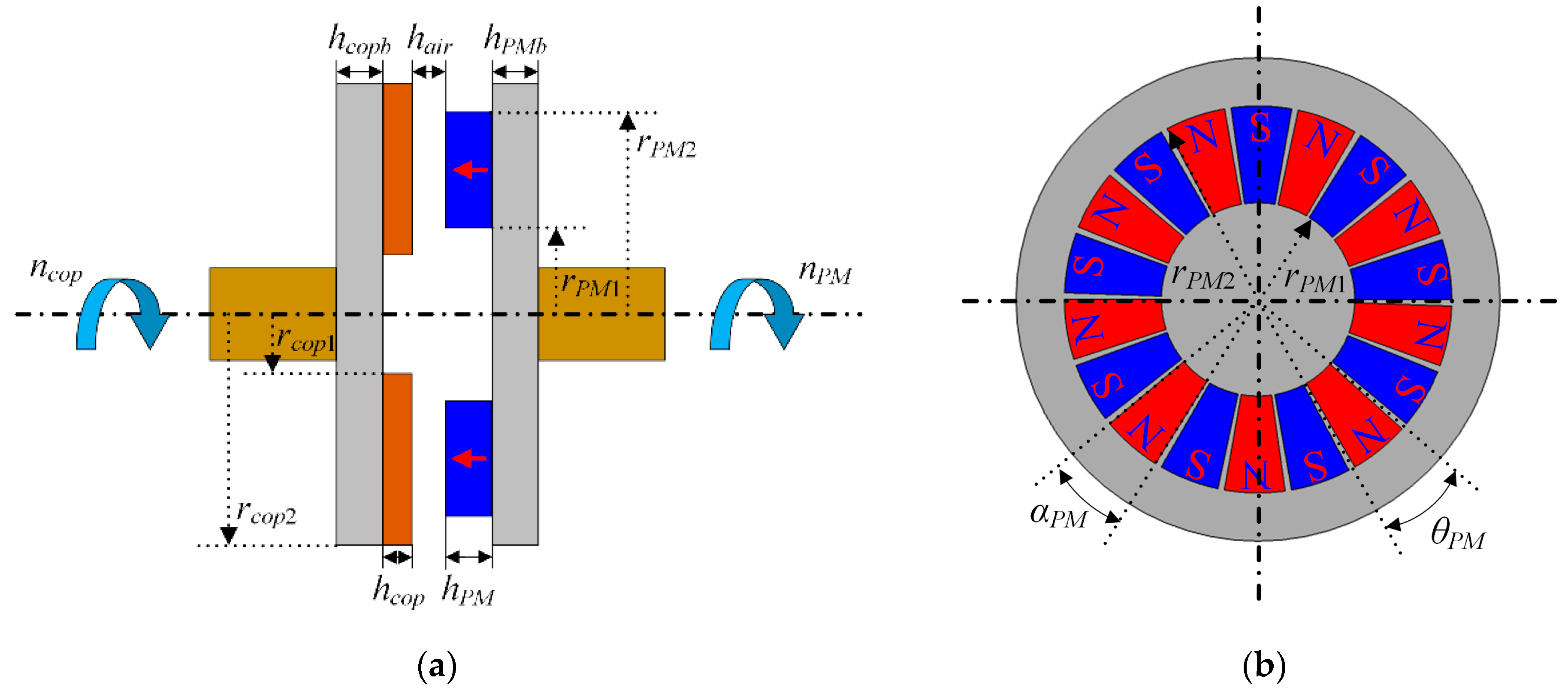
2.2. Geometries and Topologies

The geometrical parameters and a cross-section schematic of the APMC extending along the circumference are shown in Figure 2. The structural parameters h, r, and n in Figure 2 denote thickness, radius, and rotational speed, respectively. The subscripts cop, PM, air, copb, PMb, cop1, cop2, PM1, and PM2 represent the copper plate, PM, air gap, copper plate back-iron, PM back-iron, copper plate inner side, copper plate outer side, PM inner side, and PM outer side, respectively. Moreover, α_PM is the angle of the PMs in the circumferential direction, N and S are the north and south poles of the PMs, and θ_PM is the angle of the 1/2 pole pitch.

2.3. Programming of Magnetic Flux Paths

The 2D finite element qualitative simulation results for the APMC are presented in Figure 3 to intuitively visualize the magnetic flux distribution and rationally plan the magnetic circuit. As shown in Figure 3, the APMC exhibits a typical axisymmetric structure, so only the magnetic flux paths under the pair of poles need to be planned: the main magnetic circuit (solid green line) passes through the copper rotor back-iron, copper rotor, air gap, PM rotor, and PM back-iron, forming a closed loop. The magnetic flux paths consisting of the adjacent PMs, PM, and its back-iron and the copper rotor and its back-iron are all leakage magnetic flux paths (dashed blue line). In particular, the induced eddy current within the copper rotor is indicated in Figure 3 with red dots and cross symbols. The magnetic flux paths generated by the eddy current effect are represented by the long dashed red line, which passes through the conductor region and forms a closed magnetic circuit within the air gap and back-iron. The magnitude of the eddy current reaction varies with slip. In the case of high slip, the proportion of magnetic flux generated by the eddy currents is significant to the total leakage magnetic flux [4,24].

The sector-shaped PMs can not only provide a larger magnetic flux cross-sectional area S_PM but also ensure that the pole-arc coefficients at different radii are the same, thus eliminating numerous approximations and greatly improving the accuracy of the model. They can also be equivalent to other shapes of PMs with the same area and thickness, such as circular or rectangular PMs [2].

$${\alpha }_{PM}=\frac{\pi \alpha }{p}=\alpha {\theta }_{PM}$$

(1)

$$S_{PM}=\frac{{\alpha }_{PM}}{2}(r_{PM2}^2-r_{PM1}^2)$$

(2)

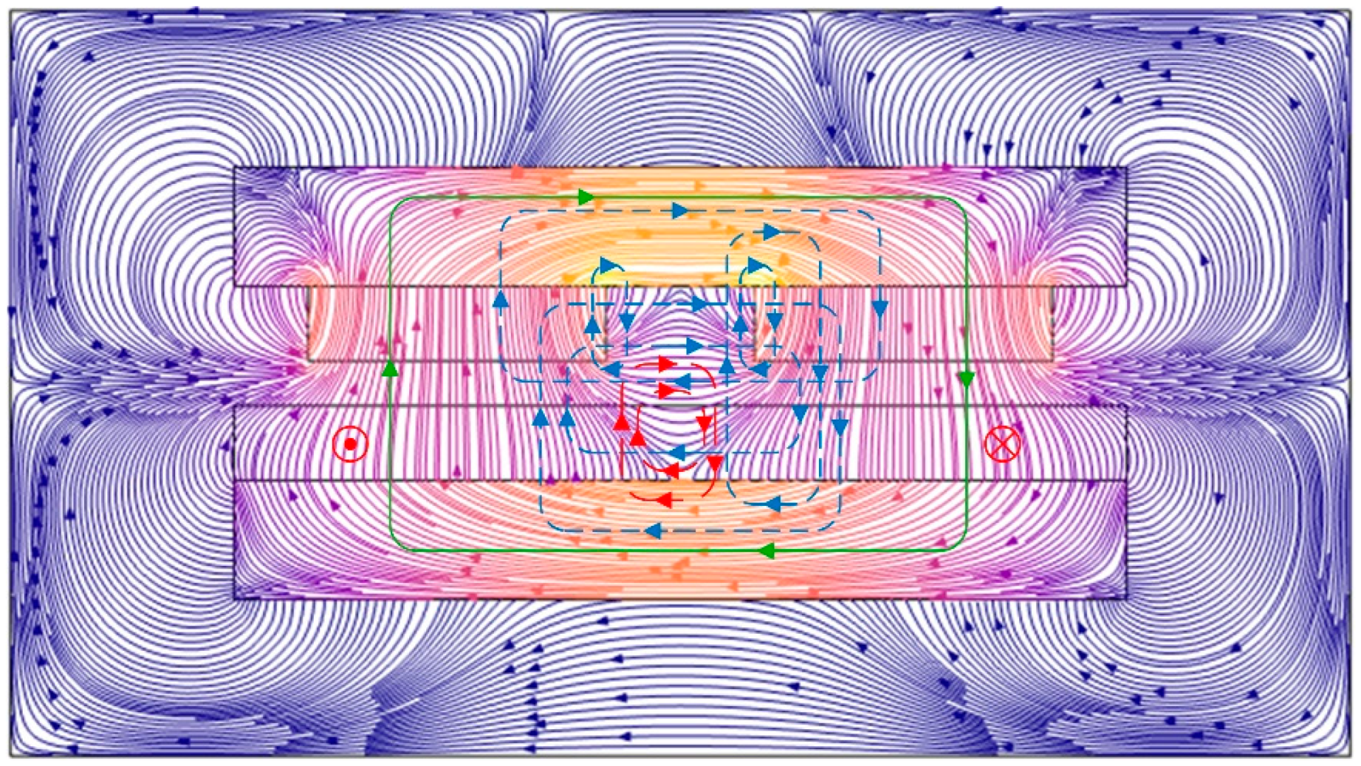
2.4. Equivalent Magnetic Circuit Method

The EMC can consider material properties such as iron saturation, remanence, and coercivity, as well as the complex geometry of the device. However, this method can only be derived under a steady state. Under dynamic conditions, the varying eddy current inside the conductor rotor excites alternating magnetic fields, causing inductive properties to be manifested, rather than purely resistive ones. Thus, a method based on sinusoidal steady-state circuits is no longer applicable.

2.4.1. Novel Equivalent Magnetic Circuit Model

Based on the symmetrical structure of the APMC and the magnetic circuit analysis, an initial EMC model for a half-pole pair shown in Figure 4 is established, where the red dashed line represents the branch magnetic circuit of the eddy current effect. The expressions for PM magnetic flux Φ_PM and magnetic resistance R_PM can be derived. The eddy current circuit contains two parts of magnetic resistance corresponding to the output power (defined as R_out) and slip power (defined as R_slip), as well as the magnetic inductance M_L corresponding to the changing magnetic field.

$${\mathrm{\Phi }}_{PM}=B_{PM}{S}_{PM}$$

(3)

$$R_{PM}=\frac{h_{PM}}{{\mu }_0{\mu }_r{S}_{PM}}$$

(4)

where B_PM, μ₀, and μ_r are the residual magnetic flux density, vacuum permeability, and relative permeability of the PMs, respectively.

In Ref. [24], the magnetic resistance is neglected by assuming an infinite magnetic permeability for the PM back-iron. Although this assumption simplifies the analysis of the moving eddy current problem, it overlooks the influence of the back-iron magnetic flux on the device performance, thereby reducing the accuracy of the model [25].

The arrangement characteristics of axially magnetized PMs are fully considered in this paper, and the back-iron magnetic resistance corresponding to the PMs and the air gap are set, respectively. Based on the power relationships of the APMC in the eddy current path, the magnetic resistance is divided into two parts, corresponding to the output power and slip power [26]. Furthermore, by reasonably transforming the EMC shown in Figure 4, a more analytically favorable Figure 5 is obtained. In Figure 5, the red dashed box still represents the eddy current effect.

The EMC model established at the average radius treats the axial magnetic flux of APMC as a linear actuator, neglecting the curvature effect and the edge effect [23]. The curvature effect primarily manifests in the leakage flux between the adjacent PMs. In previous studies, researchers attempted to calculate the magnetic flux at each radius using modulation functions and then superimpose it in the radial direction. However, there are two drawbacks to employing modulation functions, which can be referred to in Ref. [27]. To avoid repetition, the calculation details will not be reiterated here.

The edge effect will appear near the inner and outer radii of the sector-shaped PMs, resulting in a reduction in the no-load magnetic flux, which is manifested as a saddle-shape defect in the magnetic density waveform at the inner and outer radii [27]. In this paper, the concept of an edge coefficient β is proposed to reduce the influence of the edge effect on the model accuracy, and a strict definition of β is required to avoid distorted magnetic flux paths caused by an excessive air gap length in the non-magnetic regions, which leads to prolonged magnetic circuits and a weakened effective magnetic flux.

$$\beta =1+\frac{\left(r_{cop2}-r_{cop1}\right)-\left(r_{PM2}-r_{PM1}\right)}{4}$$

(5)

$$R_{ac}=\frac{h_{ac}}{{\mu }_0{\beta }^2{S}_{PM}}$$

(6)

where R_ac and h_ac are the magnetic resistance and thickness of the air gap–copper plate, respectively.

Based on the 2D finite element qualitative simulation results of the APMC as shown in Figure 3, the leakage magnetic flux paths and the integral paths are investigated. Figure 6 depicts the leakage magnetic flux between the adjacent PM surfaces and the leakage magnetic flux between the PM surface and its back-iron, respectively. It can be observed that the integral path of the leakage magnetic flux between the adjacent PM surfaces includes a straight segment and two arc segments within the air gap. The integral path of each leakage magnetic flux between the PM surface and its back-iron consists of a straight line segment and an arc segment in the air gap [28]. The magnetic resistance R_adj between the adjacent PMs and the magnetic resistance R_PMb between the PM surface and its back-iron are given in (7) and (8), where r_av is the average radius of the PMs.

$$\frac{1}{R_{adj}}=\frac{{\mu }_0(r_{PM2}-r_{PM1})}{\pi }\ln \left(\frac{{\theta }_{PM}+{\alpha }_{PM}}{{\theta }_{PM}-{\alpha }_{PM}}\right)$$

(7)

$$\frac{1}{R_{PMb}}=\frac{2{\mu }_0(r_{PM2}-r_{PM1})}{\pi }\ln \left(1+\frac{\pi r_{av}{\alpha }_{PM}}{2\left(\pi h_{air}+h_{PM}\right)}\right)$$

(8)

Due to the tight connection between the PMs and the back-iron, the magnetic flux density distribution of the latter is significantly uneven. To effectively distinguish the magnetic flux in different areas, the magnetic resistance of the back-iron is equated to a series connection of three parts, as shown in Figure 6. Consequently, the total magnetic resistance and source flux of the parallel magnetic circuit in Figure 6 can be obtained smoothly.

$$R_{b-sum}=R_{b-air}+2R_{b-PM}$$

(9)

$$R_{b-air}=\frac{r_{av}({\theta }_{PM}-{\alpha }_{PM})}{{\mu }_0{\mu }_{b-air}{h}_{PMb}(r_{PM2}-r_{PM1})}$$

(10)

$$R_{b-PM}=\frac{{\alpha }_{PM}{\theta }_{PM}{r}_{av}}{{\mu }_0{\mu }_{b-PM}\left({\alpha }_{PM}{\theta }_{PM}{r}_{av}/2+h_{PMb}\right)(r_{PM2}-r_{PM1})}$$

(11)

$$R_{par}=\frac{2R_{adj}{R}_{PMb}\left(4R_{PM}+R_{b-sum}\right)}{2R_{adj}{R}_{PMb}+\left(4R_{PM}+R_{b-sum}\right)\left(2R_{PMb}+R_{adj}\right)}$$

(12)

$${\mathrm{\Phi }}_{es}=\frac{2{\mathrm{\Phi }}_{PM}{R}_{ac}}{4R_{PM}+R_{b-sum}}$$

(13)

In (9)~(13), the magnetic resistances R_b-sum, R_b-air, R_b-PM, and R_par associated with the PMs correspond to the total back-iron, air gap–back-iron, PM–back-iron, and parallel magnetic resistance, respectively. Φ_es is the source magnetic flux of the PMs.

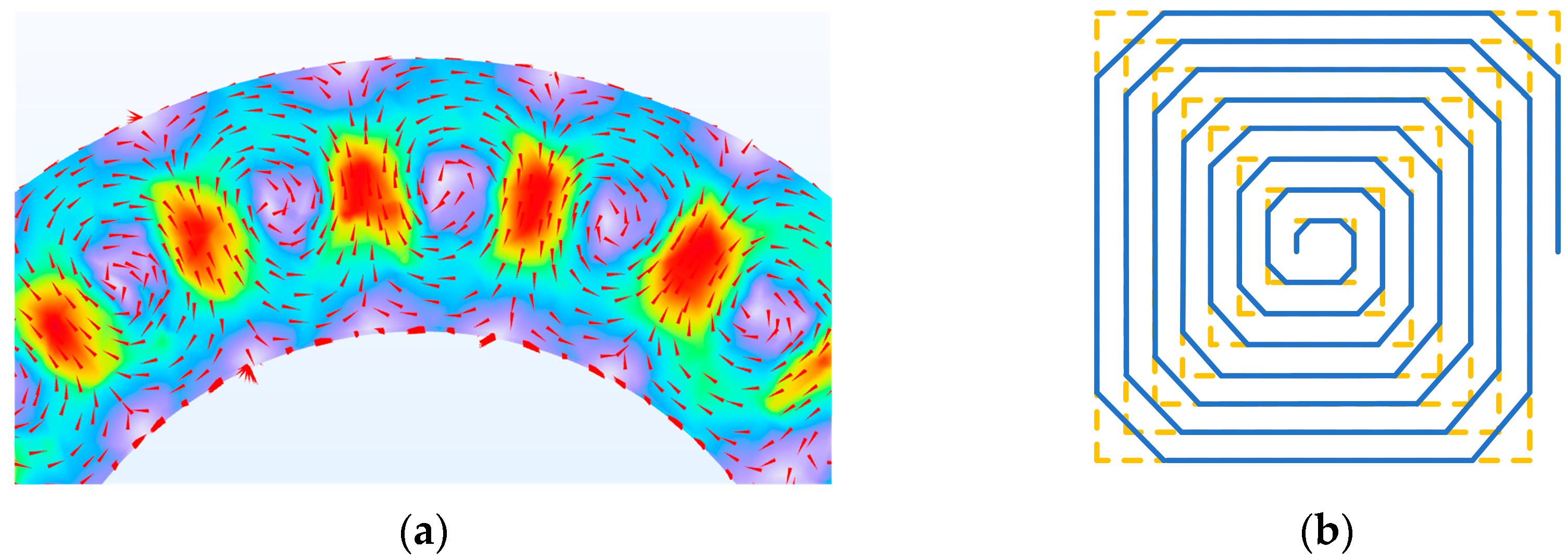
2.4.2. Eddy Current Circuit Modeling

According to Ampere’s law, the magnetic flux Φ_cop, magnetic flux density B_cop, and average eddy current density J_cop within the copper can be expressed as follows [29].

$${\mathrm{\Phi }}_{cop}=\frac{2R_{par}{C}_{av}{S}_{PM}{\mathrm{\Phi }}_{es}}{C_{av}{S}_{PM}\left(R_{par}+4R_{ac}\right)+{\mu }_0{\mu }_r{S}_{av}{R}_{par}{\sigma }_{cop}{h}_{cop}{\alpha }_{PM}{r}_{av}}$$

(14)

In Equation (14), σ_cop, s, and n_cop are the conductivity, slip, and rotational speed of the copper rotor, respectively. C_av and S_av correspond to the perimeter and area at the average radius of the sector-shaped PM.

$$B_{cop}=\frac{2{\mathrm{\Phi }}_{cop}}{S_{PM}}$$

(15)

$$J_{cop}=\frac{2{\sigma }_{cop}{v}_{re}{\mathrm{\Phi }}_{cop}}{S_{PM}}$$

(16)

$$S_{av}=\frac{{\alpha }_{PM}{r}_{av}^2}{2}$$

(17)

$$C_{av}=\pi \left(r_{PM2}+r_{PM1}\right)$$

(18)

$$v_{re}=\frac{C_{av}s{n}_{cop}}{60}$$

(19)

According to the previous analysis, it is known that there is a correspondence between the eddy current circuit and the PMs. Using the concept of the edge coefficient proposed in this paper to define the equivalent size of the eddy current circuit (equivalent area S_eddy in Equation (20) and equivalent length L_eddy in Equation (21) of the eddy current path), the eddy current, which is difficult to describe using a physical model, are expressed parametrically, so that the eddy current circuit can be modeled and calculated in a completely new way.

$$S_{eddy}={\beta }^2{S}_{PM}$$

(20)

$$L_{eddy}={\beta }^2{L}_{PM}$$

(21)

$$I_{eddy}=\frac{J_{cop}{h}_{cop}{\alpha }_{PM}{r}_{av}}{2}$$

(22)

$${\mathrm{\Phi }}_{eddy}=\frac{{\mu }_0{\mu }_r{S}_{eddy}{I}_{eddy}}{L_{eddy}}$$

(23)

The 3D finite element simulation results of the magnetic flux and corresponding eddy current density on the surface of the copper rotor at a slip speed of 100 rpm are shown in Figure 7.

It can be seen from the results that the eddy currents distributed along the radial direction in the copper plate excite the magnetic field and form a closed loop with the PMs in the main magnetic circuit to generate the output torque. The magnetic flux varies periodically with the arrangement of PMs, and the number of eddy current circuits is also the same as the number of PMs. The eddy currents distributed along the circumference, although they excite the magnetic field, do not contribute to the output torque but generate heat, corresponding to the eddy current losses.

The relative velocity v_re can be expressed more intuitively as Equation (24). By applying Equations (16) and (20)–(24), the relationship between the magnetic fluxes Φ_eddy and Φ_cop can be obtained in Equation (25). Obviously, the magnetic flux Φ_eddy under steady-state conditions is also a function of the rotational speed difference (n_cop-n_PM), which is of great significance for solving the dynamic output torque.

$$v_{re}=\frac{30\left(n_{cop}-n_{PM}\right)}{\pi r_{av}}$$

(24)

$${\mathrm{\Phi }}_{eddy}=\frac{30{\mu }_0{\mu }_r{h}_{cop}{\alpha }_{PM}{\sigma }_{cop}\left(n_{cop}-n_{PM}\right)}{\pi L_{PM}}{\mathrm{\Phi }}_{cop}$$

(25)

The magnetic resistance R_slip is established using the eddy current I_eddy and the magnetic flux Φ_eddy of the eddy current circuit based on Kirchhoff’s law, and the magnetic resistance R_out is further obtained according to the power relationship.

$$R_{slip}=\frac{s\left(2{\mathrm{\Phi }}_{cop}{R}_{ac}-I_{eddy}\right)}{{\mathrm{\Phi }}_{eddy}}$$

(26)

$$R_{out}=\frac{1-s}{s}{R}_{slip}$$

(27)

In fact, the existing research results are unable to describe the eddy currents accurately, which is a core factor limiting the modeling accuracy of the APMC. This paper attempts to model the eddy current circuit and parameterize the magnetic flux paths from the perspective of an EMC. According to Faraday’s law of electromagnetic induction, eddy currents are excited on the conductor when they cut through the rotating magnetic field of the PM rotor. The changing magnetic field will generate an induced electromotive force to resist the variation in the closed loop, causing the inductive characteristics of the conductor. The inductive characteristics are an inherent property of the closed circuit and should not be ignored.

This paper combines both field and circuit theories to develop a quantity that can describe the inductive characteristics, called the magnetic inductance M_L. Equation (25) reflects the relationship between Φ_eddy and Φ_cop under steady-state conditions, while they will be redistributed into Φ_eddy′ and Φ_cop′ due to the presence of M_L under dynamic conditions. Ohm’s law of magnetic circuits is introduced into Figure 5 and Equation (28) is given. The differential dΦ_eddy′/dt in Equation (28) can be converted into the differential of the rotational speed difference over time according to Equation (25). Moreover, this conversion can enable a measurable dynamic torque to be obtained.

$$4R_{ac}\frac{{\mathrm{\Phi }}_{cop}{}^{\prime }}{2}=\left(R_{slip}+R_{out}\right){\mathrm{\Phi }}_{eddy}{}^{\prime }+M_L\frac{d{\mathrm{\Phi }}_{eddy}{}^{\prime }}{dt}$$

(28)

The physical rules do not depend on the choice of measurement units, and the application of dimensional analysis allows for the exploration of this invariance, so as to deeply reflect the intrinsic relationships among physical quantities. Via dimensional analysis of Equation (28), the expression of M_L is reversely derived: M_L can be equivalent to the ratio of time t to inductance L.

Ref. [30] takes square inductors as an example to establish the closed form expression of inductance. The difference from other modeling methods is that the inductance calculation is based on the average segment interactions, rather than summing the individual segment interactions one by one. Hence, the total inductance consists of self-inductance and mutual inductance, including all negative and positive interactions between all segments. It should be noted that there are just the geometry parameters but no unphysical fitting factors in the model.

There is a lack of modeling for magnetic induction in existing EMCs. Therefore, the idea of modeling square inductors in Ref. [30] is extended to model the magnetic inductance of the APMC eddy current circuit shown in Figure 8a. The eddy current path is modeled as the n-turn polygonal symmetric spiral shape shown in Figure 8b. Considering the convenience of modeling, a single-turn eddy current is divided into eight segments at the average radius in Figure 8b. Of course, any position and any number of segments can be applied.

At the average radius, the length of the octagonal spiral is C_av, and then the self-inductance of the straight segment shown in Equation (7) of Ref. [30] can be obtained. Equation (29) is defined as the total square inductor length in Equations (8) and (9) in Ref. [30], since 45°-inclined segments can be decomposed into their vertical and horizontal contributing components. Therefore, the total inductance L of an octagonal spiral with a length of C_av is Equation (30). The relationship between time and relative velocity shown in Equation (31) can be obtained according to Equation (28). Based on the above analysis, the expression of M_L shown in Equation (32) can be obtained from Equations (30) and (31).

$$l_{seg}=4\times \left(\frac{C_{av}}{8}+\frac{C_{av}}{8}\sin 45°+\frac{C_{av}}{8}\cos 45°\right)=1.21C_{av}$$

(29)

$$\begin{array}{l}L=\frac{{\mu }_0{C}_{av}}{2\pi }\left(\ln \frac{C_{av}}{h_{cop}+r_{av}{\alpha }_{PM}/2}-0.9\right)-0.47\frac{{\mu }_0}{2\pi }{l}_{seg}\\ =\frac{{\mu }_0{C}_{av}}{2\pi }\left(\ln \frac{C_{av}}{h_{cop}+r_{av}{\alpha }_{PM}/2}-0.5687\right)\end{array}$$

(30)

$$t=\frac{r_{av}{v}_{re}}{n_{cop}-n_{PM}}=\frac{30}{\pi }$$

(31)

$$M_L=\frac{60}{{\mu }_0{C}_{av}\left(\ln \frac{C_{av}}{h_{cop}+r_{av}{\alpha }_{PM}/2}-0.5687\right)}$$

(32)

The parallel magnetic resistance of the two branches in Figure 5 is defined as R_// in Equation (33). The redistributed magnetic fluxes Φ_eddy′ and Φ_cop′ can be solved by constructing the magnetic circuit Equation (34) and associating it with Equation (28).

$$R_{//}=\left(4R_{PM}+R_{b-sum}\right)//\left(2R_{PMb}//R_{adj}\right)$$

(33)

$$\left({\mathrm{\Phi }}_{es}-{\mathrm{\Phi }}_{eddy}{}^{\prime }-{\mathrm{\Phi }}_{cop}{}^{\prime }\right)R_{//}=4R_{ac}\frac{{\mathrm{\Phi }}_{cop}{}^{\prime }}{2}$$

(34)

2.4.3. Calculation of Eddy Current Losses and Torque

It can be observed from Equation (28) that the magnetic inductance and magnetic resistance of a conductor represent two different energy exchange modes. The magnetic field generated by the induced current serves as the carrier of energy, making the magnetic inductance an energy storage element. The conductor plate, on the other hand, is a metal with a certain conductivity, resulting in heat generation and power losses, making the magnetic resistance an energy dissipation element. The eddy current loss P_eddy and output torque T can be further obtained by applying the above model, which does not ignore the contribution of the eddy currents in the back-iron. The detailed derivation process has been provided in Appendix A.

$$P_{eddy}=\frac{2p{\sigma }_{cop}{v}_{re}^2{h}_{cop}{\left({\mathrm{\Phi }}_{eddy}{}^{\prime }+{\mathrm{\Phi }}_{cop}{}^{\prime }/2\right)}^2}{S_{PM}}$$

(35)

$$T=\frac{2p{\sigma }_{cop}{v}_{re}{r}_{av}{h}_{cop}{\left({\mathrm{\Phi }}_{eddy}{}^{\prime }+{\mathrm{\Phi }}_{cop}{}^{\prime }/2\right)}^2}{S_{PM}}$$

(36)

3. Verification and Discussion for Proposed Model

3.1. Description of 3D Finite Element Model

A 3D finite element model based on Table 1 is conducted to verify the accuracy of the EMC model, and the meshes are divided according to the materials of each part of the APMC and their influence on the magnetic field. Figure 9 shows the division of 969,944 elements using a fixed calculation method, which allows for the simulation of the magnetic field and output torque separately, collecting more actual results that are difficult to acquire experimentally.

3.2. Parameter Sensitivity Analysis

In this section, the structural parameters of the APMC in Table 1 are used as benchmarks to investigate the effects of the conductor plate thickness, air gap thickness, and number of pole pairs on the device performance. The parameter sensitivity analysis on the one hand verifies the effectiveness and accuracy of the proposed method by establishing a 3D finite element model and an experimental prototype. On the other hand, it provides a research basis and reference data for optimizing the design.

3.2.1. Torque–Slip Speed Characteristics Related to Conductor Plate Thickness

The conductor plate serves as a carrier for eddy currents, which directly influence the eddy currents and torque. In practice, it is impossible to make the conductor plate infinitely large considering the material costs and device volume. Therefore, the thickness of the conductor plate becomes one of the important constraints in optimization tasks.

Figure 10 makes an arithmetic progression with 2 mm to 16 mm as the interval and 2 mm as the common difference to study the torque variation under different conductor plate thicknesses. In general, the torque increases significantly when increasing the slip speed and conductor plate thickness. At low slip, the effective magnetic field in the air gap mainly comes from the permanent magnetic field of the PMs, and the increase in the conductor plate thickness leads to an increase in the leakage magnetic flux, which reduces the effective magnetic field in the air gap. As the slip increases gradually, the induced magnetic field excited by eddy currents and the effective magnetic field in the air gap increase with the increase in the conductor plate thickness, manifested as the increase in torque. However, when the conductor plate thickness increases to a certain value, the growth rate of torque decreases at the same slip speed. Therefore, the relationship between the conductor plate thickness and the device volume cost should be considered comprehensively in the design and optimization of the APMC, so as to obtain the optimal matching scheme.

3.2.2. Torque–Slip Speed Characteristics Related to Air Gap Thickness

As mentioned above, the APMC realizes torque regulation by changing the thickness of the air gap between the conductor and PMs, which in turn regulates the output speed of the device, i.e., it is used as a governor. Figure 11 shows the analytical and finite element calculation results of the torque and errors at different slip speeds with air gap thicknesses of 1 mm, 3 mm, and 5 mm, respectively. It can be seen that the error between the analytical and finite element results is larger when the air gap thickness is 1 mm at low slip speeds. The reason is that when the air gap thickness and slip speed are both very small, the main magnetic circuit will experience relatively severe distortion, which makes the difference between the two calculation results larger. Therefore, in order to ensure a stable output performance in practical applications, the air gap thickness is generally controlled to be around 3 mm without being too small.

3.2.3. Eddy Current Loss–Slip Speed Characteristics Related to Air Gap Thickness

The results of the analytical and finite element calculations of the eddy current losses under different air gap thicknesses and the error between the two methods corresponding to Figure 11 are shown in Figure 12. The error is larger for an air gap thickness of 5 mm at low slip speed. The reason for this situation is that the eddy current mainly generates losses in the form of heat. When the air gap thickness is relatively large, the magnetic resistance of the air gap and the energy consumption increase, which ultimately leads to the deviation of the calculation results. Other than that, the errors of the analytical and finite element calculation results fluctuate within an acceptable small range, proving that the model proposed in this paper can calculate the eddy current losses accurately.

3.2.4. Torque–Slip Speed Characteristics Related to the Number of Pole Pairs

The establishment of the initial magnetic field and the generation of eddy currents in the APMC all originate from the PMs. The number of pole pairs of the PMs determines the distribution and periodicity of the magnetic field in the air gap and the eddy currents in the conductor plate, which plays a decisive role in the output performance: it is then one of the most important design parameters of the device. The output torque characteristic curves for the number of pole pairs vary from 6 to 11 and are given in Figure 13. It can be seen that the output torque increases with an increase in the number of pole pairs, but the growth rate decreases. In other words, there must be a critical pole pair value so that the torque no longer increases with the number of pole pairs. In addition, PMs cannot be used in large quantities due to their expensive prices in practical engineering applications. Therefore, it is particularly important to balance the relationship between the number of PMs and output performance in the optimization of APMCs.

3.2.5. Dynamic Torque Characteristics

The dynamic torque characteristics of the APMC at an air gap thickness of 2 mm and different slip speeds are shown in Figure 14. The startup process of the APMC is essentially the establishment and action process of the magnetic field. At the initial stage, there are no eddy currents inside the copper rotor. The increasing slip speed causes the eddy currents to gradually increase, and the output torque also increases accordingly. However, the torque will not reach its maximum immediately due to the magnetic resistance of the copper rotor. Ultimately, the output torque will achieve dynamic stability.

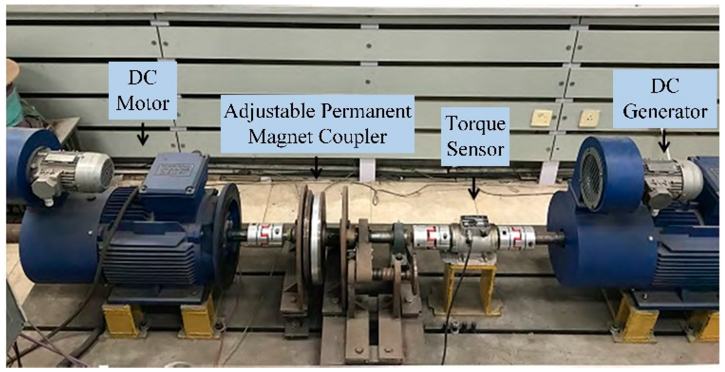
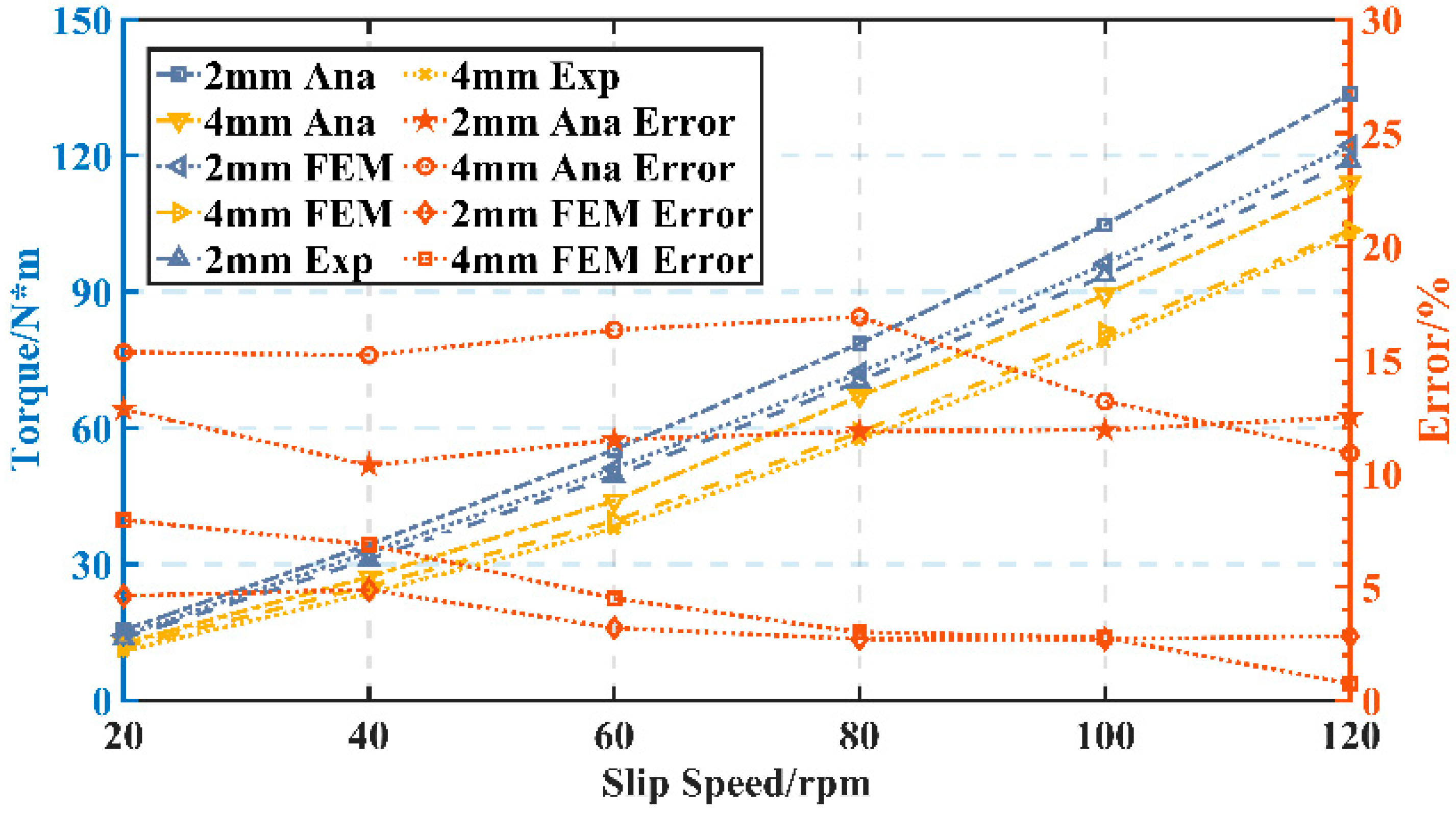
3.3. Experimental Prototype Validation

The experimental prototype was manufactured based on the structural parameters shown in Table 1 to verify the accuracy of torque, and an experimental platform as shown in Figure 15 was built. The platform consists of a drag motor, an APMC prototype, and a generator. To measure the output torque of the drag motor and the rotational speed of the load, a torque–speed sensor is installed between the APMC and the load generator. The speed of the drag motor is measured using an encoder mounted on it. The measurement data collected by the torque–speed sensor and the encoder can be uploaded to a computer for storage.

The measured torque characteristic curves of the prototype at the air gap thicknesses of 2 mm and 4 mm and their error curves with analytical and finite element methods are given in Figure 16. According to the experimental results, it can be concluded that: (1) The increase in the air gap thickness significantly reduces the output torque at the same slip speed. (2) The error rate of the two methods is within 18%; although they are relatively accurate, there is still great room for improvement. (3) The 3D FEM is more consistent with the actual test results with an error rate of 5–8%. Therefore, in the absence of a measured prototype, the results of the 3D FEM can serve as a verification benchmark, which provides convenience for the optimization of the device. (4) The possible sources of the errors are mainly the influence of the conductor plate temperature rise on the characteristics of the APMC and the deviation generated by the sensor data.

4. Conclusions and Future Highlights

A novel parameterized EMC modeling method for an APMC is proposed in this paper. According to the electromagnetic coupling characteristics of the APMC, the resistance and inductance characteristics of the conductor eddy current loop are introduced into the EMC model as a branch circuit. The analytical method based on the EMC makes the performance prediction for the APMC simple and practical. The concept of the edge coefficient effectively reduces the edge effect near the inner and outer radii of the sector-shaped PMs without 3D correction. The magnetic flux, magnetic resistance, and eddy current density of each branch magnetic circuit are established under steady-state conditions. The concept of magnetic inductance is first proposed to parameterize eddy currents that are difficult to accurately describe using physical models. On this basis, Ohm’s law of a dynamic eddy current circuit is established to obtain the dynamic eddy current model. In addition, the magnetic resistance is subdivided into two parts corresponding to the output and slip according to the power relationship, from which the eddy current loss and dynamic torque models are further derived. The method proposed in this paper is verified by comparing the analytical prediction with the finite element calculation. It can achieve satisfactory results within a reasonable range of slip speed and structural parameters. The method proposed in this paper is suitable for different PM geometries, thus providing a theoretical basis for the design and optimization of the APMC. Compared with existing analytical methods, the EMC is easy to program and implement, and the calculation process is short, making it very suitable for the initial design stage of devices. The processing technology regarding the eddy current branch also provides a feasible method for effectively evaluating the EMC modeling, including the induced eddy current problem of the moving conductors.

The method proposed in this paper is a bold attempt and breakthrough of an EMC for an APMC. The parameter sensitivity analysis verifies the validity and accuracy of the method in terms of the conductor plate thickness, air gap thickness, and number of pole pairs. The 3D finite element simulation model and experimental prototype further demonstrate the reliability of the analytical method in modeling the APMC. However, concerns are expressed about the shortcomings of its generalization capability, which will be the motivation of and main work for further exploration in the future.

References

1. Ye, L.; Li, D.; Ma, Y.; Jiao, B. Design and Performance of a Water-Cooled Permanent Magnet Retarder for Heavy Vehicles. IEEE Trans. Energy Convers. 2011, 26, 953–958. [Google Scholar] [CrossRef]
2. Wang, J.; Lin, H.; Fang, S.; Huang, Y. A General Analytical Model of Permanent Magnet Eddy Current Couplings. IEEE Trans. Magn. 2014, 50, 1–9. [Google Scholar] [CrossRef]
3. Atallah, K.; Wang, J. A Brushless Permanent Magnet Machine with Integrated Differential. IEEE Trans. Magn. 2011, 47, 4246–4249. [Google Scholar] [CrossRef]
4. Yang, X.; Liu, Y.; Wang, L. Nonlinear Modeling of Transmission Performance for Permanent Magnet Eddy Current Coupler. Math. Probl. Eng. 2019, 2019, 1–14. [Google Scholar] [CrossRef]
5. Shin, H.-J.; Choi, J.-Y.; Jang, S.-M.; Lim, K.-Y. Design and Analysis of Axial Permanent Magnet Couplings Based on 3D FEM. IEEE Trans. Magn. 2013, 49, 3985–3988. [Google Scholar] [CrossRef]
6. Potgieter, J.H.J.; Kamper, M.J. Optimum Design and Comparison of Slip Permanent-Magnet Couplings with Wind Energy as Case Study Application. IEEE Trans. Ind. Appl. 2014, 50, 3223–3234. [Google Scholar] [CrossRef]
7. Gay, S.E.; Ehsani, M. Parametric Analysis of Eddy-Current Brake Performance by 3-D Finite-Element Analysis. IEEE Trans. Magn. 2006, 42, 319–328. [Google Scholar] [CrossRef]
8. Canova, A.; Cavalli, F. Design Procedure for Hysteresis Couplers. IEEE Trans. Magn. 2008, 44, 2381–2395. [Google Scholar] [CrossRef]
9. Zhang, B.; Wan, Y.; Li, Y.; Feng, G. Optimized Design Research on Adjustable-Speed Permanent Magnet Coupling. In Proceedings of the 2013 IEEE International Conference on Industrial Technology (ICIT), Cape Town, South Africa, 25–28 February 2013; IEEE: New York, NY, USA, 2013; pp. 380–385. [Google Scholar]
10. Erasmus, A.S.; Kamper, M.J. Analysis for Design Optimisation of Double PM-Rotor Radial Flux Eddy Current Couplers. In Proceedings of the 2015 IEEE Energy Conversion Congress and Exposition (ECCE), Montreal, QC, Canada, 20–24 September 2015; IEEE: New York, NY, USA; pp. 6503–6510. [Google Scholar]
11. Canova, A.; Vusini, B. Design of Axial Eddy-Current Couplers. IEEE Trans. Ind. Appl. 2003, 39, 725–733. [Google Scholar] [CrossRef]
12. Canova, A.; Vusini, B. Analytical Modeling of Rotating Eddy-Current Couplers. IEEE Trans. Magn. 2005, 41, 24–35. [Google Scholar] [CrossRef]
13. Shin, H.-J.; Choi, J.-Y.; Cho, H.-W.; Jang, S.-M. Analytical Torque Calculations and Experimental Testing of Permanent Magnet Axial Eddy Current Brake. IEEE Trans. Magn. 2013, 49, 4152–4155. [Google Scholar] [CrossRef]
14. Park, M.-G.; Choi, J.-Y.; Shin, H.-J.; Jang, S.-M. Torque Analysis and Measurements of a Permanent Magnet Type Eddy Current Brake with a Halbach Magnet Array Based on Analytical Magnetic Field Calculations. J. Appl. Phys. 2014, 115, 17E707. [Google Scholar] [CrossRef]
15. Lubin, T.; Rezzoug, A. Steady-State and Transient Performance of Axial-Field Eddy-Current Coupling. IEEE Trans. Ind. Electron. 2015, 62, 2287–2296. [Google Scholar] [CrossRef]
16. Lubin, T.; Rezzoug, A. 3-D Analytical Model for Axial-Flux Eddy-Current Couplings and Brakes Under Steady-State Conditions. IEEE Trans. Magn. 2015, 51, 1–12. [Google Scholar] [CrossRef]
17. Lubin, T.; Rezzoug, A. Improved 3-D Analytical Model for Axial-Flux Eddy-Current Couplings with Curvature Effects. IEEE Trans. Magn. 2017, 53, 1–9. [Google Scholar] [CrossRef]
18. Jang, G.-H.; Koo, M.-M.; Kim, J.-M.; Choi, J.-Y. Torque Characteristic Analysis and Measurement of Axial Flux-Type Non-Contact Permanent Magnet Device with Halbach Array Based on 3D Analytical Method. AIP Adv. 2017, 7, 056647. [Google Scholar] [CrossRef]
19. Lubin, T.; Mezani, S.; Rezzoug, A. Two-Dimensional Analytical Calculation of Magnetic Field and Electromagnetic Torque for Surface-Inset Permanent-Magnet Motors. IEEE Trans. Magn. 2012, 48, 2080–2091. [Google Scholar] [CrossRef]
20. Sheikh-Ghalavand, B.; Vaez-Zadeh, S.; Hassanpour Isfahani, A. An Improved Magnetic Equivalent Circuit Model for Iron-Core Linear Permanent-Magnet Synchronous Motors. IEEE Trans. Magn. 2010, 46, 112–120. [Google Scholar] [CrossRef]
21. Qu, R.; Lipo, T.A. Analysis and Modeling of Air-Gap and Zigzag Leakage Fluxes in a Surface-Mounted Permanent-Magnet Machine. IEEE Trans. Ind. Appl. 2004, 40, 121–127. [Google Scholar] [CrossRef]
22. Momen, M.F.; Datta, S. Analysis of Flux Leakage in a Segmented Core Brushless Permanent Magnet Motor. IEEE Trans. Energy Convers. 2009, 24, 77–81. [Google Scholar] [CrossRef]
23. Aberoomand, V.; Mirsalim, M.; Fesharakifard, R. Design Optimization of Double-Sided Permanent-Magnet Axial Eddy-Current Couplers for Use in Dynamic Applications. IEEE Trans. Energy Convers. 2019, 34, 909–920. [Google Scholar] [CrossRef]
24. Wang, J.; Zhu, J. A Simple Method for Performance Prediction of Permanent Magnet Eddy Current Couplings Using a New Magnetic Equivalent Circuit Model. IEEE Trans. Ind. Electron. 2018, 65, 2487–2495. [Google Scholar] [CrossRef]
25. Lubin, T.; Mezani, S.; Rezzoug, A. Simple Analytical Expressions for the Force and Torque of Axial Magnetic Couplings. IEEE Trans. Energy Convers. 2012, 27, 536–546. [Google Scholar] [CrossRef]
26. You, S.-A.; Wang, S.-H.; Tsai, M.-C.; Mao, S.-H. Characteristic Analysis of Slotted-Type Axial-Flux Permanent Magnetic Couplers. In Proceedings of the 2012 15th International Conference on Electrical Machines and Systems, Sapporo, Japan, 21–24 October 2012; p. 5. [Google Scholar]
27. de la Barriere, O.; Hlioui, S.; Ben Ahmed, H.; Gabsi, M.; LoBue, M. 3-D Formal Resolution of Maxwell Equations for the Computation of the No-Load Flux in an Axial Flux Permanent-Magnet Synchronous Machine. IEEE Trans. Magn. 2012, 48, 128–136. [Google Scholar] [CrossRef]
28. Chen, J.T.; Zhu, Z.Q. Influence of the Rotor Pole Number on Optimal Parameters in Flux-Switching PM Brushless AC Machines by the Lumped-Parameter Magnetic Circuit Model. IEEE Trans. Ind. Appl. 2010, 46, 1381–1388. [Google Scholar] [CrossRef]
29. Yang, F.; Zhu, J.; Yang, C.; Ding, Y.; Hang, T. A Simple Method to Calculate the Torque of Magnet-Rotating-Type Axial Magnetic Coupler Using a New Magnetic Equivalent Circuit Model. IEEE Trans. Magn. 2022, 58, 1–12. [Google Scholar] [CrossRef]
30. Jenei, S.; Nauwelaers, B.; Decoutere, S.; Nacm, A. Closed form inductance calculation for integrated spiral inductor compact modeling. In Proceedings of the 2000 Topical Meeting on Silicon Monolithic Integrated Circuits in Rf Systems, Digest of Papers, Garmisch Partenki, Germany, 26–28 April 2000. [Google Scholar]
Figure 1. Two types of APMC: (a) excitation in axial direction; (b) excitation in radial direction.
Mathematics 11 04793 g001
Figure 2. Geometrical parameters and cross-section schematic of APMC: (a) axial topology of APMC; (b) circumferential distribution of PMs.
Mathematics 11 04793 g002
Figure 3. Planning of magnetic flux paths.
Mathematics 11 04793 g003
Figure 4. Initial EMC model.
Mathematics 11 04793 g004
Figure 5. Simplified EMC model.
Mathematics 11 04793 g005
Figure 6. Magnetic flux paths of leakage flux.
Mathematics 11 04793 g006
Figure 7. FEM results of magnetic flux and eddy current on the surface of copper rotor.
Mathematics 11 04793 g007
Figure 8. Eddy current path and octagonal spiral model of APMC: (a) eddy current path based on COMSOL; (b) octagonal spiral model.
Mathematics 11 04793 g008
Figure 9. Mesh partition model based on FEM.
Mathematics 11 04793 g009
Figure 10. Torque–slip speed characteristics related to conductor plate thickness.
Mathematics 11 04793 g010
Figure 11. Torque–slip speed characteristics related to air gap thickness.
Mathematics 11 04793 g011
Figure 12. Eddy current loss–slip speed characteristics related to air gap thickness.
Mathematics 11 04793 g012
Figure 13. Torque–slip speed characteristics related to number of pole pairs.
Mathematics 11 04793 g013
Figure 14. Dynamic torque characteristics.
Mathematics 11 04793 g014
Figure 15. The experimental platform of APMC.
Mathematics 11 04793 g015
Figure 16. Torque-slip speed characteristics related to air gap thickness.
Mathematics 11 04793 g016