Article

Dimensionality Reduction with Variational Encoders Based on Subsystem Purification

1
Department of Physics and Astronomy, Purdue University, West Lafayette, IN 47907, USA
2
Department of Chemistry, Purdue University, West Lafayette, IN 47907, USA
3
Oak Ridge National Laboratory (ORNL), Oak Ridge, TN 37830, USA
4
Purdue Quantum Science and Engineering Institute, West Lafayette, IN 47907, USA
*
Author to whom correspondence should be addressed.
Mathematics 2023, 11(22), 4678; https://doi.org/10.3390/math11224678
Submission received: 26 October 2023 / Revised: 13 November 2023 / Accepted: 15 November 2023 / Published: 17 November 2023
(This article belongs to the Special Issue Quantum Algorithms and Quantum Computing)

Abstract

:
Efficient methods for encoding and compression are likely to pave the way toward the problem of efficient trainability on higher-dimensional Hilbert spaces, overcoming issues of barren plateaus. Here, we propose an alternative approach to variational autoencoders to reduce the dimensionality of states represented in higher dimensional Hilbert spaces. To this end, we build a variational algorithm-based autoencoder circuit that takes as input a dataset and optimizes the parameters of a Parameterized Quantum Circuit (PQC) ansatz to produce an output state that can be represented as a tensor product of two subsystems by minimizing T r ( ρ 2 ) . The output of this circuit is passed through a series of controlled swap gates and measurements to output a state with half the number of qubits while retaining the features of the starting state in the same spirit as any dimension-reduction technique used in classical algorithms. The output obtained is used for supervised learning to guarantee the working of the encoding procedure thus developed. We make use of the Bars and Stripes (BAS) dataset for an 8 × 8 grid to create efficient encoding states and report a classification accuracy of 95% on the same. Thus, the demonstrated example provides proof for the working of the method in reducing states represented in large Hilbert spaces while maintaining the features required for any further machine learning algorithm that follows.
MSC:
81P68

1. Introduction

Variational quantum algorithms in the NISQ [1] era provide a promising route toward developing useful algorithms that allow for optimizing states in higher dimensional spaces by tuning the polynomial number of parameters. The most prominent techniques within variational methods include the Variational Quantum Eigensolver (VQE) [2], Quantum Approximate Optimization Algorithm (QAOA) [3], and other classical machine learning-inspired ones. We ask the readers to refer to [4] for an exhaustive study on quantum machine learning with applications in chemistry [5], physics [6], supervised learning and optimization [7]. Within the context of optimization and machine learning in general, some of the major problems that need to be addressed include encoding classical data, finding an expressible enough ansatz (Expressibility) [8], and efficiently computing gradients (Trainability) [9], generalizability [10]. These problems are interlinked and thus not treated independently in general.
As we move away from the NISQ era toward deep parameterized quantum circuits (PQC), one of the major problems with regard to trainability that needs addressing is the problem of vanishing gradients referred to as barren plateaus [11]. This might be an effect of working with a large number of qubits [11], expressive circuit ansatz [12], noise inducement [13] or the use of global cost functions in the learning [14]. Having efficient procedures to reduce the dimensionality the representation of the input quantum state helps create efficient encoding schemes that could later be used as inputs to other machine learning algorithms, where the cost functions on higher dimensional spaces with expressive ansatz are less likely to be trainable. To this end, we develop machine learning techniques that allow for compact representations of a given input quantum state.
Within the classical machine learning community, autoencoders have been effectively used to develop low-dimensional representation of samples generated from a given probability distribution [15]. Inspired by these techniques, work on Quantum Autoencoders [16,17] have allowed for people to develop compact representations against a fixed finite state. It is not clear that such tensor product states with a fixed finite state are always possible while retaining the maximal possible information. Here, we show that if one were to relax the condition toward maintaining a fixed finite state, a better compact representation can be generated that can be post-processed toward classification. We develop techniques to create subsystem purifications for a given set of inputs and follow it by creating superpositions of these purifications indexed using the subsystem number. This representation is further used for doing classification achieved by applying variational methods over parameterized quantum circuits restricted to this compact representation and showing the learning of the method. We apply an ansatz to create subsystem purification on the Bars and Stripes (BAS) dataset and show that one can reduce the number of qubits required to represent the data by half and achieve a 95% classification accuracy on the Bars and Stripes (BAS) dataset. The demonstrated example shows proof for the working of the method in reducing states represented in large Hilbert spaces while maintaining the features required for any further machine learning algorithm that follows. The scheme thus proposed can be extended to problems with states in large Hilbert spaces where dimensionality reduction plays a key role with regard to the trainability of the parameterized quantum circuit.

2. Method

Given an ensemble of input states, E = { | ψ i } , the objective is to construct a low-dimensional representation of states sampled from this distribution E. Let | ψ i be a state over n A + n B qubits. We design a protocol that allows for us to create an equivalent compact representation of | ψ with m a x ( n A , n B ) + 1 qubits. To simplify the discussion, let us assume that n A = n B , and thus, we create a representation using half the qubits. We do this in 2 stages.
Stage 1:
In the first stage, we apply a unitary U ( θ ) that decomposes | ψ i A , B into | α ( θ ) i A | β ( θ ) i B . To produce such a tensor product structure, we could minimize the entropy on either subsystem A or B till a zero entropy is achieved. Thus, we could optimize the cost function,
C B ( θ ) = S t r A U ( θ ) | ψ A B ψ | A B U ( θ ) { | ψ }
where t r A represents the tracing operation over the qubits of subsystem A, < . > { | ψ } represents the averaging over the { | ψ } , and S ( ρ ) = t r ( ρ l o g ( ρ ) ) is the entropy of a given density matrix ρ . The cost function C B ( θ ) attains a maximum value equal to l o g ( n B ) when ρ B is maximally mixed and equal to 0 when ρ B is in a pure state. Figure 1 shows a schematic representation of the ansatz used for U ( θ ) . The hardware efficient ansatz used here is restricted to R y gates on each qubit followed by a ladder of CNOT operators that couples adjacent qubits. This is sufficient for our purpose as the input data vectors used here, associated with bars and stripes, are vectors with real amplitudes.
Variational quantum algorithms have been studied in the past to create thermal systems by minimizing the free energy of the output state [18,19]. The main problem tackled in these papers involves developing techniques that allow one to compute the gradients of Entropy required to be optimized over the training. The issue arises from not having exact representations that can compute the logarithm of a given density matrix efficiently. Furthermore, to avoid numerical instabilities in the entropy function arising from the density matrix of pure states being singular, here, we alternatively maximize over the cost function,
C A B ( θ ) = 1 2 T r A ( ρ A 2 ) + T r B ( ρ B 2 ) { | ψ }
where ρ A = T r B ( U ( θ ) | ψ A B ψ | A B U ( θ ) ) and ρ B = T r A ( U ( θ ) | ψ A B ψ | A B U ( θ ) ) . C A B attains a maximum value of 1 when ρ A or ρ B are pure states resulting in T r ( ρ A / B 2 ) = T r ( ρ A / B ) = 1 and attains a least value 2 / 2 n . C A B is a convex function as T r ( ρ A / B 2 ) is a convex function of ρ A / B [18]. Figure 2 shows a schematic representation to compute T r ( ρ 2 ) using a destructive swap test. The optimization landscape thus has one local minimum dictated by the expressivity of the ansatz used to capture it.
The parameters θ are variationally optimized to obtain θ * = argmax θ C A B ( θ ) . If C A B ( θ ) reaches an optimal value of zero, we can express | ψ A B = | ϕ A | η B , thus expressing a state with 2 n + m degrees of freedom, effectively using 2 n + 2 m degrees of freedom. Having expressed the input state as a tensor product of subsystems, we now move to stage 2 of the algorithm.
Stage 2:
Note that the above representation still makes use of 2 n qubits to capture the features of | ψ . If the subsystems are not equal in size, additional ancillary qubits are included to match the system size. We now show how this representation can be compressed using n + 1 qubits. To carry this out, we apply an ancillary CSWAP (controlled swap/Fredkin) gate acting on the qubits of systems A and B. The additional ancillary qubit works as an index register for these states. Thus, we obtain | 0 | ϕ | η + | 1 | η | ϕ . If | η and | ϕ are not orthogonal states, then there exists at least one basis element | g in the computational basis with a nonzero coefficient in both these states. Without a loss of generality, let us assume that the measurement collapses onto | g , giving rise to 1 1 + c 2 ( | 0 | ϕ + c e i α | 1 | η ) | g , where c and α are real numbers. The factor c e i α is generated from the relative difference in the coefficients of the state corresponding to | g . Figure 3 shows a schematic representation of the main steps involved in creating a superposition, with the ancilla register being used as an index to the subsystem outputs of Stage 1.
Output:
Thus, we have successfully managed to map the input state | ψ to 1 1 + c 2 ( | 0 | ϕ + c e i α | 1 | η ) , apart from an arbitrary relative phase ϕ and amplitude c in the representation. Note that this procedure is reversible, thus preserving all information content encoded into input state | ψ . To show that it is reversible, one just needs to take two copies of the output state 1 1 + c 2 ( | 0 | ϕ + c e i α | 1 | η ) , measure the corresponding ancilla to project out | ϕ | η , and then apply the inverse of U ( θ ) , giving back | ψ . Thus, the encoding scheme allows for us to create a representation of the input state | ψ with 2 n qubits into only n + 1 qubits. We now show that the presence of the arbitrary phase and relative coefficient can be ignored if we work with an ansatz with a specific structure for an L2 cost function, which can be generalized to other cost functions as well.
Let V ( α ) be the ansatz used for classification after creating the compact state representation. We calculate the label corresponding to each state by averaging the expectation value across an ensemble of representative states for each datapoint obtained via projection of the second state. The expected label for a datapoint indexed by t is thus given by
Expected Label = i P ( i ) ψ ˜ i , t | V ( α ) [ Z I n ] V ( α ) | ψ ˜ i , t
where i indexes the projection of the second subsystem and P ( i ) is the probability of that projection. Using the L2 norm, the classification cost function with respect to this ansatz is given by
Classification Cost = t ( l t i P ( i ) ψ ˜ i , t | V ( α ) [ Z I n ] V ( α ) | ψ ˜ i , t ) 2
where | ψ = 1 1 + c 2 ( | 0 | ϕ + c e i α | 1 | η ) . Note here V ( α ) is an ansatz that acts on n + 1 qubits. The cost expression chosen abive can be re-expressed on the non-projected state as follows:
Classification Cost = t ( l t ψ | V ( α ) I n [ Z I n I n ] V ( α ) I n | ψ ) 2
where | ψ = | 0 | ϕ | η + | 1 | η | ϕ . The above extension is supported by the presence of P ( i ) in the original expression. We now choose an ansatz that allows us to get rid of the effects of arbitrary relative phase and amplitude via the projection of the second subsystem in our original expression. Let V ( α 1 , α 2 ) = | 0 0 | V 0 ( α 0 ) + | 1 1 | V 1 ( α 1 ) , where α = ( α 0 , α 1 ) . Thus we obtain
Classification Cost = t ( l t ϕ | V 0 ( α 0 ) [ Z I n 1 ] V 0 ( α 0 ) | ϕ η | V 1 ( α 1 ) [ Z I n 1 ] V 1 ( α 1 ) | η ) 2
The above expression thus obtained is akin to the averaging over the ensemble for each datapoint producing a state that is oblivious to the relative amplitude and phase factor produced via the projection. For both V 0 ( α 0 ) and V 1 ( α 1 ) , we use the hardware efficient ansatz, as shown in Figure 1, which we shall employ for supervised learning in the next section.

3. Results

To demonstrate the working of the method described above, we pick a toy dataset with images of Bars and Stripes (BAS) and build a compact representation of it. The BAS dataset we consider is a square grid with either some columns being only vertically filled (Bars) or some rows being horizontally filled (Stripes) [21]. One can easily generate such a supervised dataset and realize that the distribution from which these images are sampled has a low entropy characterization. We randomly sample 1000 data points from a grid size of 16 × 16 from the BAS dataset consisting of 131,068 datapoints represented using amplitude encoding on eight qubits. Note that, despite other classically trained and more efficient encodings that could be straightforwardly employed, here, we use amplitude encoding, as the representation is efficient in the number of qubits while remaining data-agnostic.
Applying the protocol described above, we reduce the representation of the state into a tensor product of two subsystems of equal size. 
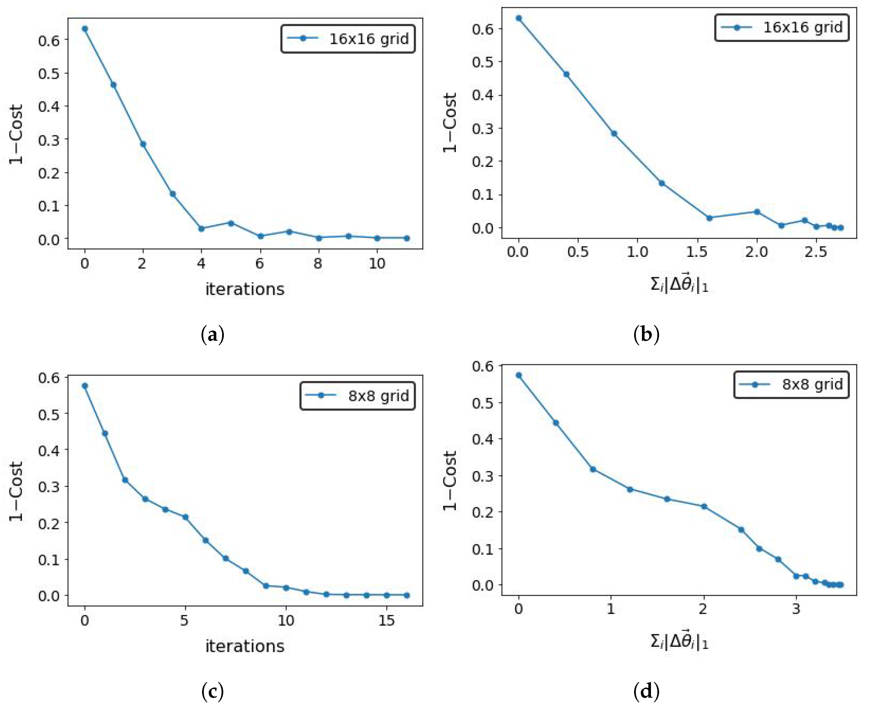
Figure 4 shows the learning of optimal parameters θ as the cost function falls. Note that the dataset has been factorized from a non-trivially entangled state. We use the standard gradient descent [22] approach in performing the training. Note that the cost function drops to zero, implying that the representation thus created is exact with a lossless transformation created by U ( θ ) . For the 16 × 16 grid case, the ansatz U ( θ ) is made of D = 5 layers, while that for the 8 × 8 grid is made of D = 3 layers. At this point, we apply a layer of swap gates to reduce the eight-qubit representation of 16 × 16 grid samples into five qubits and the six-qubit representation of 8 × 8 grid samples into four qubits.
We now use this as input for performing supervised classification. We use approximately 80% of the samples from the output of the encoded samples for training and keep the remaining 20% of the samples for testing. An ansatz V ( α 1 , α 2 ) = | 0 0 | V 0 ( α 0 ) + | 1 1 | V 1 ( α 1 ) with the same number of qubits as that of the input samples is trained, with the expectation value of pauli-Z operator being used as a label for differentiating between bars and stripes. The input image is classified as an image of bars if the expectation value is positive and as stripes image if it is negative. We use the sum of two norm errors over the dataset labels (1 for bars and 1 for stripes) as the cost function (6) to be minimized over, i.e,
Classification Cost = t ( l t ϕ | V 0 ( α 0 ) [ Z I n 1 ] V 0 ( α 0 ) | ϕ η | V 1 ( α 1 ) [ Z I n 1 ] V 1 ( α 1 ) | η ) 2
where the summation index i labels the dataset, l i refers to the labels corresponding to the sample input and | ψ i is used to denote the compact representation of the state that the above encoding scheme provides. For the 8 × 8 grid, a total of 508 bars and stripe images are produced, with half of them belonging to each category. We use 400 of these samples for training and 108 samples for testing. By default, we have used 8192 shots for each measurement during the training for creating subsystem purifications and carrying out the classification. We use 1000 representative samples corresponding to each datapoint, which are characterized by an arbitrary relative phase and amplitude. Figure 5 shows the cost of optimizing the parameters of V ( θ ) as a function of the number of iterations. We achieved a 95% accuracy on the testing data, showing that the method used to generate the compact representation did not destroy the features of the input state.

4. Runtime Analysis of Encoding Scheme

Here we shall analytically compute the required runtime for the protocol described above. Let us assume that the input ensemble of N quantum states over n qubits supports a compact representation, allowing us to use the above protocol to encode with half the number of qubits. Let our ansatz to be optimized be made of d layers. Thus, stage 1 involves optimization over 2 n d N parameters for N samples. Using a destructive swap test to compute fidelity with an error ϵ , we would require O ( 1 / ϵ 2 ) samples. Thus, the runtime complexity scales evaluate O ( n d N / ϵ 2 ) quantum circuits per iteration for Stage 1. Stage 2 involves sampling output states after measuring the second system in a fixed basis. If K representative samples characterized by arbitrary phase and amplitude are used for each data point, then the overall runtime is bounded by O ( K N T n d / ϵ 2 ) .

5. Discussion and Conclusions

We discuss a scheme that allows for a compact representation of states in higher-dimensional Hilbert spaces using half the number of qubits. The output thus created serves as a good starting state for any further machine learning algorithm that might follow. The protocol is based on designing a quantum circuit that allows creating a tensor product subsystems and demonstrates results on bars and stripes datasets for 8 × 8 grid and 16 × 16 grid. We further use this output to create compact representations with half the number of qubits as compared to the starting state. To show that this representation is a lossless encoding, we use it to perform supervised learning using variational circuits on the entire dataset of an 8 × 8 grid and reproduce a 95% accuracy on the training dataset (consisting of 108 samples). Unlike quantum autoencoders where the compact representations rely on being able to optimize against a fixed garbage state, here, the relaxed restriction on the tensor product helps provide compact representations in cases where a fixed garbage state would not be feasible. The protocol described works in the absence of noise, as it requires creating pure tensor product subsystems. Further future investigation with regard to how one might overcome this hurdle is required across all quantum autoencoder protocols that aspire to create efficient codes. One might also be interested in carrying out machine learning by using weighted quantum circuits that run on the subsystems independently and compare their performance against the compact representations created thereby. One can also imagine using low entropic entangled states that stage 1 protocol outputs as input states for entanglement forging [23] and look for useful applications with them. We would like to conclude by saying that efficient methods for encoding and compression are likely to pave the way toward the problem of efficient trainability on higher-dimensional Hilbert spaces, and this work serves as a step in that direction.

Author Contributions

Conceptualization, R.S. and M.S.; Validation, M.S.; Formal analysis, R.S. and M.S.; Investigation, R.S.; Resources, T.S.H.; Writing—original draft, R.S.; Visualization, S.K.; Supervision, T.S.H. and S.K.; Project administration, T.S.H. and S.K.; Funding acquisition, T.S.H. and S.K. All authors have read and agreed to the published version of the manuscript.

Funding

This material is based upon work supported by the U.S. Department of Energy, the Office of Science, the National Quantum Information Science Research Centers, and the Quantum Science Center. This manuscript has been authored by UT-Battelle, LLC under contract DE-AC05-00OR22725 with the US Department of Energy (DOE). Sabre Kais would like to acknowledge the support from the National Science Foundation under award number 1955907.

Data Availability Statement

Data are contained within the article.

Conflicts of Interest

The authors declare no conflict of interest.

References

  1. Preskill, J. Quantum computing in the NISQ era and beyond. Quantum 2018, 2, 79. [Google Scholar] [CrossRef]
  2. Peruzzo, A.; McClean, J.; Shadbolt, P.; Yung, M.H.; Zhou, X.Q.; Love, P.J.; Aspuru-Guzik, A.; O’brien, J.L. A variational eigenvalue solver on a photonic quantum processor. Nat. Commun. 2014, 5, 4213. [Google Scholar] [CrossRef]
  3. Farhi, E.; Goldstone, J.; Gutmann, S. A quantum approximate optimization algorithm. arXiv 2014, arXiv:1411.4028. [Google Scholar]
  4. Sajjan, M.; Li, J.; Selvarajan, R.; Sureshbabu, S.H.; Kale, S.S.; Gupta, R.; Singh, V.; Kais, S. Quantum machine learning for chemistry and physics. Chem. Soc. Rev. 2022, 51, 6475–6573. [Google Scholar] [CrossRef]
  5. Xia, R.; Kais, S. Quantum machine learning for electronic structure calculations. Nat. Commun. 2018, 9, 4195. [Google Scholar] [CrossRef]
  6. Selvarajan, R.; Sajjan, M.; Kais, S. Variational quantum circuits to prepare low energy symmetry states. Symmetry 2022, 14, 457. [Google Scholar] [CrossRef]
  7. Selvarajan, R.; Dixit, V.; Cui, X.; Humble, T.S.; Kais, S. Prime factorization using quantum variational imaginary time evolution. Sci. Rep. 2021, 11, 20835. [Google Scholar] [CrossRef]
  8. Sim, S.; Johnson, P.D.; Aspuru-Guzik, A. Expressibility and entangling capability of parameterized quantum circuits for hybrid quantum-classical algorithms. Adv. Quantum Technol. 2019, 2, 1900070. [Google Scholar] [CrossRef]
  9. Du, Y.; Hsieh, M.H.; Liu, T.; You, S.; Tao, D. Learnability of quantum neural networks. PRX Quantum 2021, 2, 040337. [Google Scholar] [CrossRef]
  10. Banchi, L.; Pereira, J.; Pirandola, S. Generalization in Quantum Machine Learning: A Quantum Information Standpoint. PRX Quantum 2021, 2, 040321. [Google Scholar] [CrossRef]
  11. McClean, J.R.; Boixo, S.; Smelyanskiy, V.N.; Babbush, R.; Neven, H. Barren plateaus in quantum neural network training landscapes. Nat. Commun. 2018, 9, 4812. [Google Scholar] [CrossRef]
  12. Holmes, Z.; Sharma, K.; Cerezo, M.; Coles, P.J. Connecting ansatz expressibility to gradient magnitudes and barren plateaus. PRX Quantum 2022, 3, 010313. [Google Scholar] [CrossRef]
  13. Wang, S.; Fontana, E.; Cerezo, M.; Sharma, K.; Sone, A.; Cincio, L.; Coles, P. Noise-Induced Barren Plateaus in Variational Quantum Algorithms. arXiv 2020, arXiv:2007.14384. [Google Scholar] [CrossRef]
  14. Cerezo de la Roca, M.V.S.; Sone, A.; Volkoff, T.J.; Cincio, L.; Coles, P.J. Cost function dependent barren plateaus in shallow parametrized quantum circuits. Nat. Commun. 2021, 12, 1791. [Google Scholar] [CrossRef]
  15. Kingma, D.P.; Welling, M. An Introduction to Variational Autoencoders. Found. Trends® Mach. Learn. 2019, 12, 307–392. [Google Scholar] [CrossRef]
  16. Romero, J.; Olson, J.P.; Aspuru-Guzik, A. Quantum autoencoders for efficient compression of quantum data. Quantum Sci. Technol. 2017, 2, 045001. [Google Scholar] [CrossRef]
  17. Wan, K.H.; Dahlsten, O.; Kristjánsson, H.; Gardner, R.; Kim, M. Quantum generalisation of feedforward neural networks. NPJ Quantum Inf. 2017, 3, 36. [Google Scholar] [CrossRef]
  18. Wang, Y.; Li, G.; Wang, X. Variational Quantum Gibbs State Preparation with a Truncated Taylor Series. Phys. Rev. Appl. 2021, 16, 054035. [Google Scholar] [CrossRef]
  19. Chowdhury, A.N.; Low, G.H.; Wiebe, N. A Variational Quantum Algorithm for Preparing Quantum Gibbs States. arXiv 2020, arXiv:2002.00055. [Google Scholar] [CrossRef]
  20. Cincio, L.; Subaşı, Y.; Sornborger, A.T.; Coles, P.J. Learning the quantum algorithm for state overlap. New J. Phys. 2018, 20, 113022. [Google Scholar] [CrossRef]
  21. Benedetti, M.; Garcia-Pintos, D.; Perdomo, O.; Leyton-Ortega, V.; Nam, Y.; Perdomo-Ortiz, A. A generative modeling approach for benchmarking and training shallow quantum circuits. NPJ Quantum Inf. 2019, 5, 45. [Google Scholar] [CrossRef]
  22. Wierichs, D.; Izaac, J.; Wang, C.; Lin, C.Y.Y. General parameter-shift rules for quantum gradients. Quantum 2022, 6, 677. [Google Scholar] [CrossRef]
  23. Eddins, A.; Motta, M.; Gujarati, T.P.; Bravyi, S.; Mezzacapo, A.; Hadfield, C.; Sheldon, S. Doubling the size of quantum simulators by entanglement forging. PRX Quantum 2022, 3, 010309. [Google Scholar] [CrossRef]
Figure 1. Ansatz used for the Encoding circuit U ( θ ) in stage 1. The circuit shows D repeating layers of a unit consisting of R y gates parameterized by one independent angle each and a ladder of C N O T operators. The circuit is optimized over the dataset to generate equivalent states with a subsystem tensor product structure. Thus, we obtain U ( θ ) | ψ = | ϕ | η . ϕ is the first subsystem and shall be indexed later with an ancilla state | 0 and | η is the second subsystem, which shall be indexed by | 1 .
Mathematics 11 04678 g001
Figure 2. The quantum circuit above implements a destructive swap test. Given 2 different density matrices as inputs, the circuit computes the fidelity of states F ( γ , σ ) = ( T r ( γ σ γ ) 2 , where γ and σ are 2 density matrices. Here, we use γ = σ = | ρ ρ | . Post-processing of measurements with the input as 2 copies of | ρ is used to compute T r ( ρ 2 ) [20].
Mathematics 11 04678 g002
Figure 3. A schematic representation of the steps involved in Stage 2 to prepare the superposition state using an extra ancilla from the product state output of Stage 1. Controlled swap gates are used to generate 1 1 + c 2 ( | 0 | ϕ + c e i α | 1 | η ) . Following this, the second subsystem is measured in the computational basis imparting relative phase and amplitude (not shown in the above representation).
Mathematics 11 04678 g003
Figure 4. The above graphs show the cost of training the parameters of U ( θ ) according to Equation (2) as a function of iterations and the 1 norm change in the absolute gradients for 1000 samples from a 16 × 16 grid on 8 qubits and 508 samples from 8 × 8 grid on 6 qubits. The unitary circuit thus trained creates equivalent tensor product representations using two equal half subsystems of 4 and 3 qubits for samples from the 16 and 8 grids, respectively. Notice that in (a,c), 1–Cost eventually saturates at 0, allowing us to create pure state product subsystems, while in (b,d), the variation in angle as computed using the gradient of Equation (2) is minimized as one gets near the saturation point ( | Δ θ | 1 measures the 1 norm increase in the angle contribution from the computed gradients with increasing epochs). (a) Stage 1: Training cost vs. iterations for 16 × 16 grid; (b) stage 1: Training cost vs. i | Δ θ i | 1 for 16 × 16 grid; (c) stage 1: Training cost vs. iterations for 8 × 8 grid; (d) stage 1: Training cost vs. i | Δ θ i | 1 for 8 × 8 grid.
Mathematics 11 04678 g004
Figure 5. Optimization of parameters of V ( θ ) towards classification on a compact representation of images of 8 × 8 BAS dataset generated using the variational method described above. (a) shows the saturation of classification cost as per Equation (7) after 13 iterations. (b) shows that the variation in angle as computed using the gradient of Equation (7) is minimized as one gets near the saturation point. ( | Δ θ | 1 measures the 1 norm increase in the angle contribution from the computed gradients with increasing epochs). (a) Classification cost vs. iterations for 8 × 8 grid. (b) Classification cost vs. i | Δ θ i | 1 for 8 × 8 grid.
Mathematics 11 04678 g005
Disclaimer/Publisher’s Note: The statements, opinions and data contained in all publications are solely those of the individual author(s) and contributor(s) and not of MDPI and/or the editor(s). MDPI and/or the editor(s) disclaim responsibility for any injury to people or property resulting from any ideas, methods, instructions or products referred to in the content.

