1. Introduction
Let
be a polynomial ring over a field
K with standard grading, that is,
, for all
i. Let
M be a finitely generated graded
-module. Suppose that
M admits the following minimal free resolution:
The projective dimension of
M is defined as
. The
of
M is defined to be the common length of all maximal
M-sequences in the unique graded maximal ideal
. Let
M be a finitely generated
-graded
-module. For a homogeneous element
and a subset
,
denotes the
K-subspace of
M generated by all homogeneous elements of the form
, where
v is a monomial in
. The
K-subspace,
, is called a
Stanley space of dimension
if it is a free
-module, where
denotes the number of indeterminates in
A. A
Stanley decomposition of
M is a presentation of the
K-vector space
M as a finite direct sum of Stanley spaces:
The Stanley depth of decomposition
is defined as
. The
Stanley depth of
M is defined as
Stanley conjectured in [
1] that
; this conjecture was later disproved by Duval et al. [
2] in 2016. However, it is still important to prove Stanley’s inequality for some special classes of ideals. Herzog et al. gave a method in [
3] to compute the Stanley depth of modules of the form
, where
are monomial ideals. But in general, it is still too hard to compute Stanley depth even using their method. For further details, we refer the reader to [
4,
5,
6].
Let
be a graph, where
is the vertex set and
is the edge set of graph
G. All graphs considered in this paper are simple and undirected. The edge ideal
of the graph
G is the ideal generated by all monomials of the form
such that
. In the last decade, the study of edge ideals has gained considerable attention. Various findings on these ideals have demonstrated how combinatorial and algebraic aspects interact; see, for instance, [
7,
8]. The algebraic invariant depth, Stanley depth, and projective dimension have significant importance in the field of commutative algebra. Establishing the relationship of these invariants with other invariants of commutative algebra and invariants of graph theory are current trends in research.
In general, the invariant depth, Stanley depth, and projective dimension are hard to compute. There are very few classes of ideals for which the formulae of these invariants are known; see, for instance, [
4,
9,
10]. We prove that when we consider the
r-fold graph of a ladder graph, circular ladder graph, some king’s graphs, and some circular king’s graphs, then the value of depth, Stanley depth, and projective dimension of the quotients rings of the edge ideals of these graphs are functions of
r. We also prove that Stanley’s inequality also holds for these quotient rings. Furthermore, our results give strong motivation for further studies in this direction. For our main results, see Theorem 3, Corollary 4, Theorem 4, Theorem 6, Corollary 4, and Theorem 7.
2. Preliminaries
In this section, we will recall some definitions and notations from graph theory. For terminology and definitions from graph theory, we refer the reader to [
11,
12,
13,
14]. Some known results related to depth and Stanley depth are also given in this section. If
I is a monomial ideal then
denotes its unique minimal set of monomial generators. If
u is a monomial of
, then
, and for a monomial ideal
I, we define
. The
degree of a vertex
denoted by
is the number of edges that are incident to
. Let
, a
path of length
, denoted by
, be a graph with
and
(if
, then
). Let
, a
cycle of length
denoted by
, be a graph with
and
. A graph is said to be a
tree if it is acyclic. A vertex
is called a
pendant vertex if
. For
, an
r-star denoted by
is a tree with
leaves and a single vertex with degree
. A
caterpillar is a tree in which the removal of all pendants leaves a path.
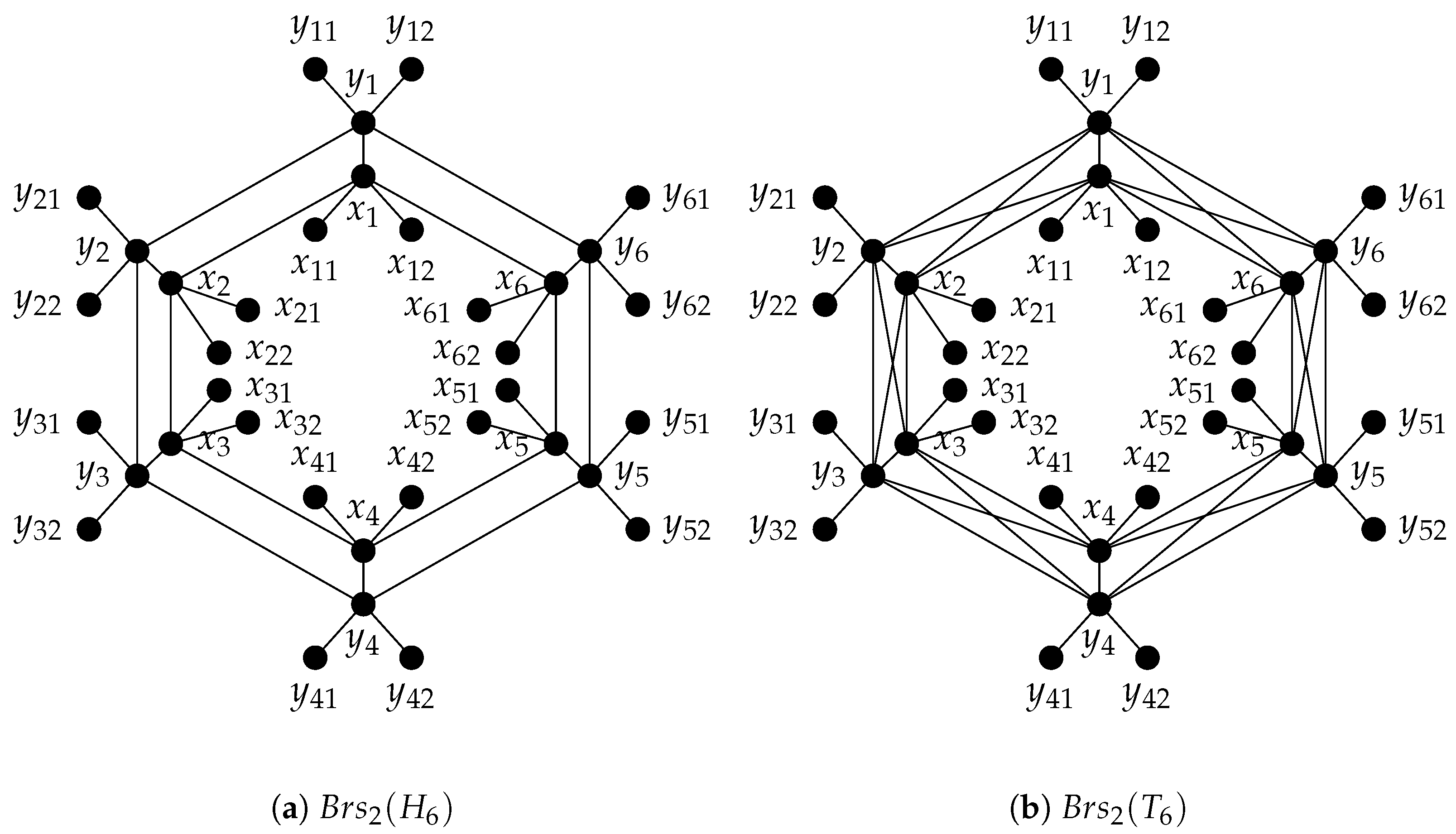
Definition 1 ([15]). Let G be a graph and be an integer. The graph obtained by attaching r pendant vertices to each vertex of G is called the r-fold bristled graph of G. The r-fold bristled graph of G is denoted by . Definition 2 ([
16])
. The Cartesian product of graphs and is a graph with vertex set and , whenever- 1.
and ;
- 2.
and .
Definition 3 ([
16])
. The strong product of graphs and is a graph with vertex set and , whenever- 1.
and ;
- 2.
and ;
- 3.
and .
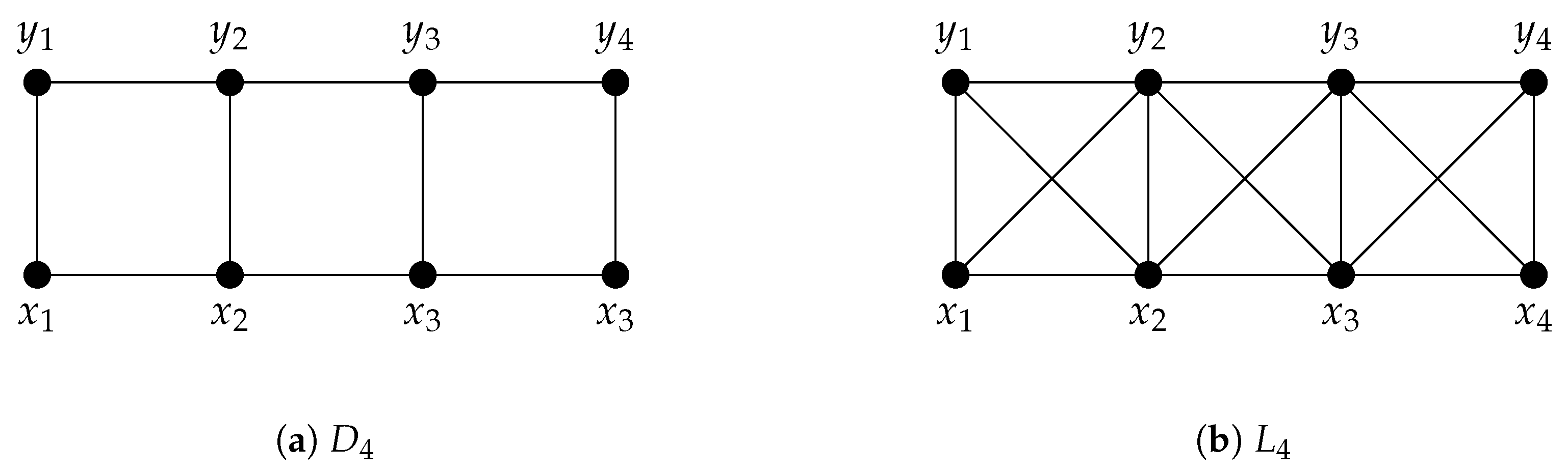
Here we introduce some notations that will be used throughout the paper. For
, let
and
be graphs. The graph
is known as a
ladder graph, whereas the graph
is called
()-king’s graph. See
Figure 1 for examples of
and
. For
, let
and
; the graph
is called a
circular ladder graph. We define the graph
as
circular ()-king’s graph.
Now we recall some known results that are frequently used in this paper. The following lemma, which is also known as the Depth Lemma, has a crucial role in all proofs of our results concerning depth.
Lemma 1 ([
17])
. If is a short exact sequence of modules over a local ring , or a Noetherian graded ring with local, then- 1.
.
- 2.
.
- 3.
.
A similar result for Stanley depth as given in the subsequent lemma is proved by Rauf.
Lemma 2 ([
18])
. Let be a short exact sequence of -graded -module. Then Here is a list of some preliminary lemmas that are referred to many times in the proofs of our results.
Lemma 3 ([
3])
. Let be a monomial ideal. If then and Lemma 4 ([
19])
. If is an edge ideal of υ-star, then Lemma 5 ([
20])
. Let , be monomial ideals, where and . Then Lemma 6 ([
20])
. Let and be monomial ideals, where and . Then The following results are useful in finding upper bounds for depth and Stanley depth.
Corollary 1 ([
18])
. Let be a monomial ideal. Then for all monomials . Proposition 1 ([
21])
. Let be a monomial ideal. Then for all monomials , Lemma 7 ([
22])
. Let be a squarefree monomial ideal with , let , such that , for all . Then The following result says that once the value of depth of a module is know then one can find its projective dimension.
Theorem 1 ([
17])
. (Auslander–Buchsbaum formula) If is a commutative Noetherian local ring and M is a non-zero finitely generated -module of finite projective dimension, then For and , if , then clearly is a caterpillar and we have the following values for depth and Stanley depth.
Theorem 2 ([
23])
. Let and . Then Throughout this paper, we set , where r and are positive integers. Also,
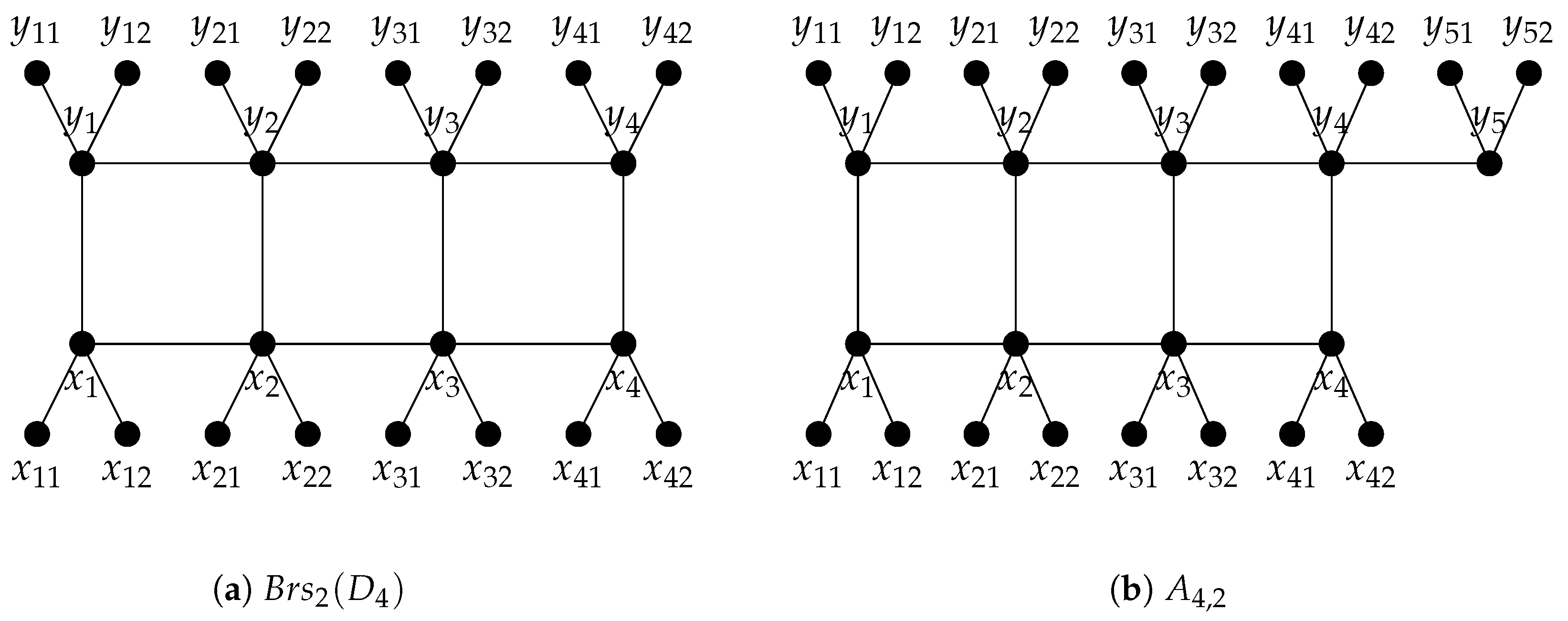
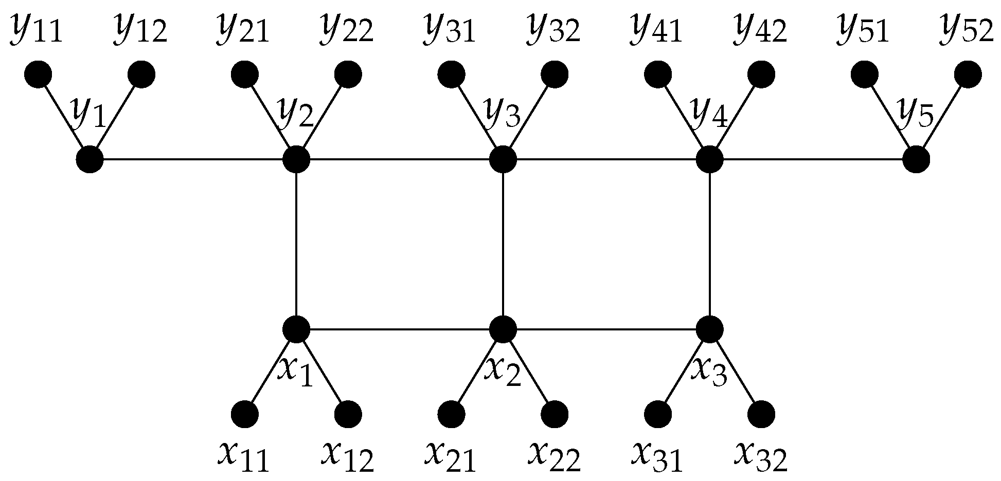
3. Depth and Stanley Depth of r-Fold Bristled Graph of Ladder Graph and Some King’s Graph
In this section, we determine depth, projective dimension, and Stanley depth of the quotient rings associated with edge ideals of
r-fold bristled graphs of graphs
and
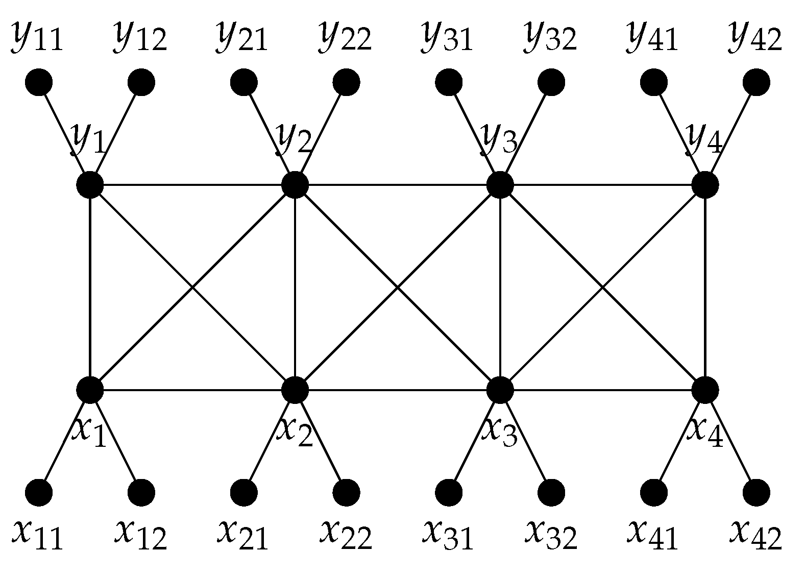
. See
Figure 2a and
Figure 3 for 2-fold bristled graph of graphs
and
, respectively. We label the vertices of
and
, as shown in
Figure 2a and
Figure 3, respectively. For
, let
and
. If
denotes the minimal set of monomial generators of the monomial ideal
I, using our labeling, we have
and
If
, then we have
and
Note that
and
. We also define a modified graph of
denoted by
with the set of vertices
and
. See
Figure 3b for an example of graph
and labeling of vertices of this graph. We set
and
. Clearly,
. Note that
,
and
. To determine depth and Stanley depth of
, we shall first determine the depth and Stanley depth of
.
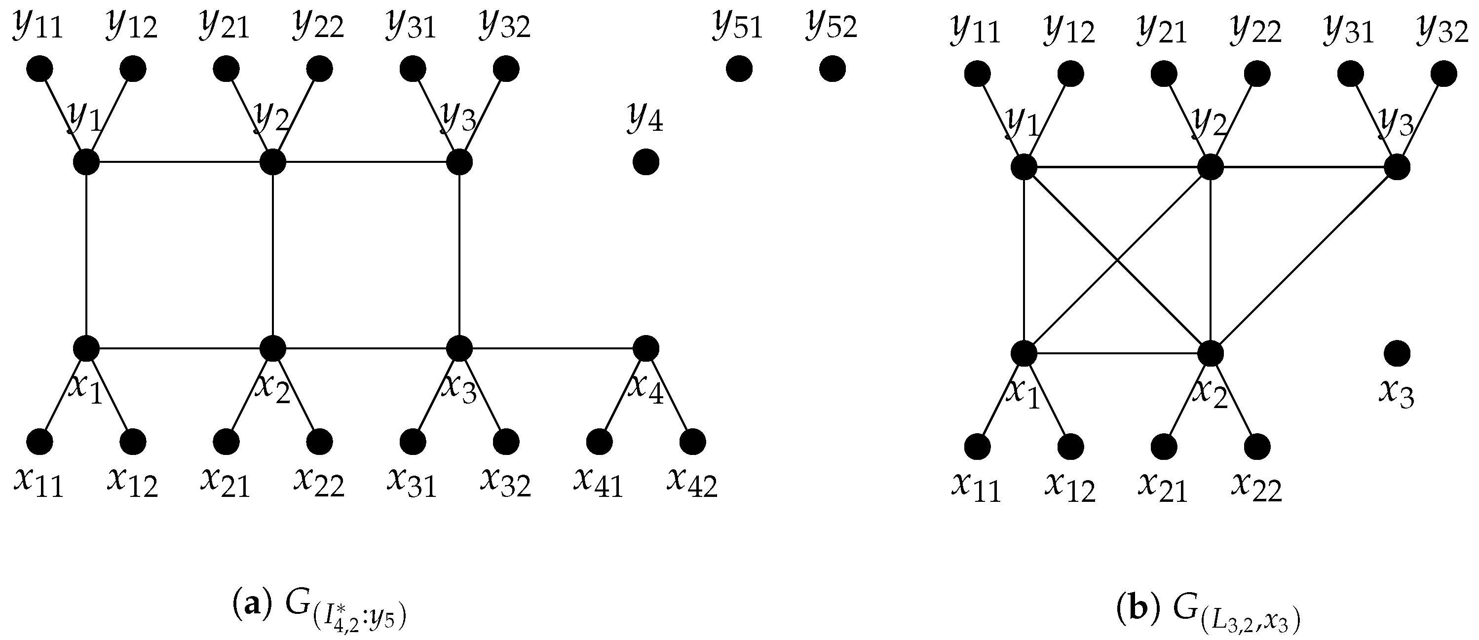
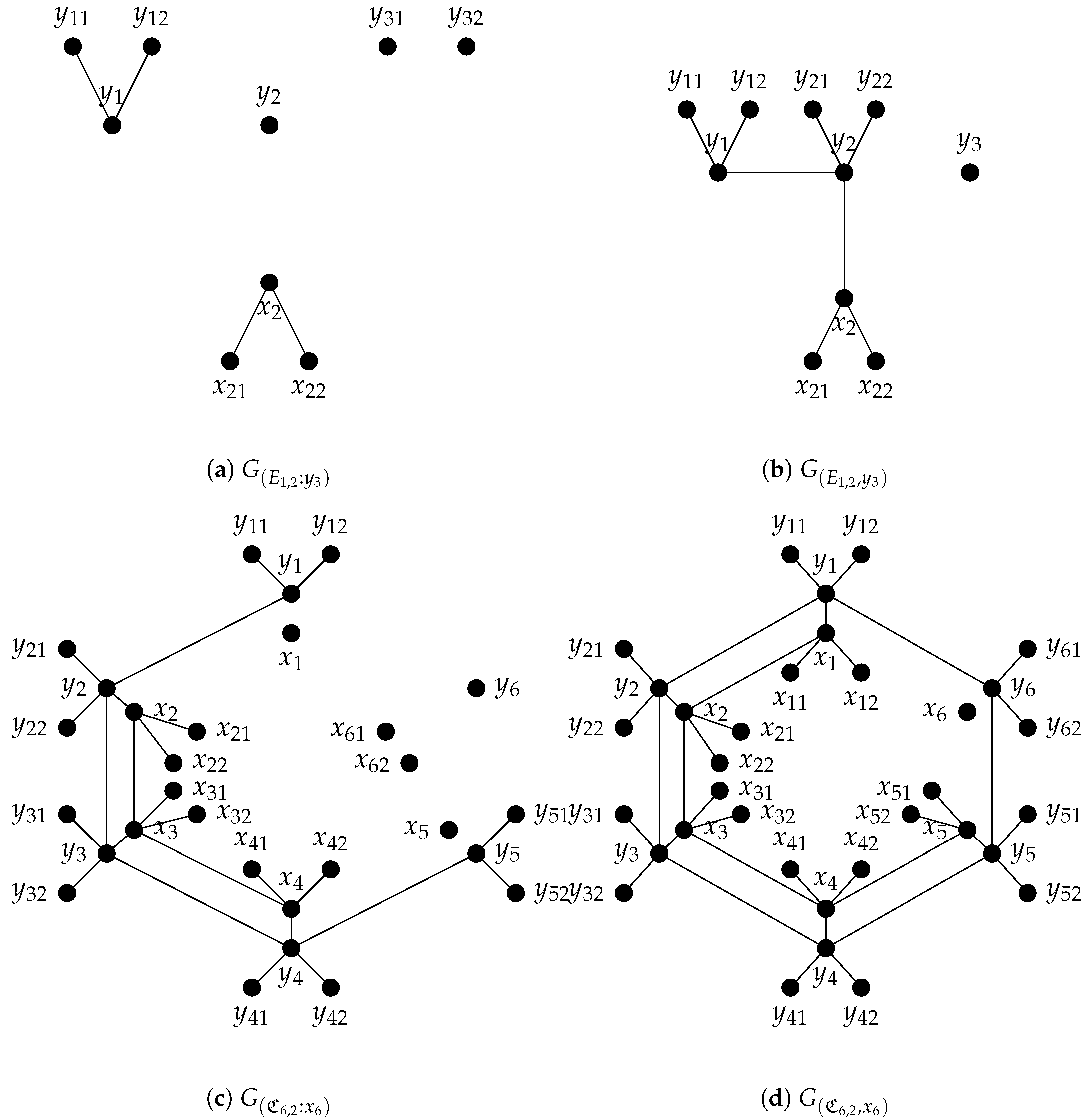
Remark 1. Let I be a squarefree monomial ideal of whose monomial generators have degrees of at most 2. We associate a graph to the ideal I with and . Let be a variable of the polynomial ring such that . Then and are monomial ideals of such that and are subgraphs of . See Figure 4a and Figure 4b for graphs and , respectively. Remark 2. While proving our results by induction on , the special cases, say and , that might appear in the proofs need to be addressed first. We define and . Thus, we have , and by Lemma 4, we have .
Lemma 8. Let . Then
Proof. First we will prove the result for depth. We will prove this by induction on
. We consider the following short exact sequence:
If
, then by Theorem 2,
, as required. Let
. After renumbering the variables, we have
Thus, by induction and Lemma 3,
Also,
Using induction and Lemma 4,
By Equation (
1), we have
Now we prove the other inequality. We have
by Lemma 3,
By induction, we have
As , so by Corollary 1 This completes the proof for depth.
Now we prove the result for Stanley depth. If , then by Theorem 2, . For , the required result follows by applying Lemma 2 instead of the Depth Lemma, Lemma 6 instead of Lemma 5, and Proposition 1 instead of Corollary 1. □
Corollary 2. Let . Then
Proof. The required result follows by using Lemma 8 and Theorem 1. □
Now using the previous lemma, we are able to prove one of the main results of this section.
Theorem 3. Let . Then
Proof. First we will prove the result for depth. Consider the following short exact sequence:
When
, it is clear from Theorem 2 that
. Let
. We have
By Lemma 3, we have
By Lemma 8,
Now clearly
and
, and using Lemma 3,
By Lemma 8,
Applying the Depth Lemma,
Now we prove the result for Stanley depth. If
, then by Theorem 2, we have
Let
. Applying Lemma 2 on the short exact sequence, we obtain
Proceeding on the same lines as we did for the depth, we obtain
and
and by Equation (
2), we have
. For the other inequality, since
and
, by Lemma 8,
By Proposition 1, we have
This completes the proof for Stanley depth. □
Corollary 3. Let . Then
Proof. The required result follows by using Theorem 3 and Theorem 1. □
Now we find the depth and Stanley depth of .
Theorem 4. Let . Then
Proof. First we will prove the result for depth. We will prove this by induction on
. Consider the following short exact sequence:
By the Depth Lemma,
When
, it is clear from Theorem 2 that
.
Let
,
Using Lemma 3 and induction on
, clearly
Now let
and
Consider the following short exact sequence:
Again, using the Depth Lemma, we have
Here
Using Lemma 3 and induction on
, we have
As
and
By Lemma 3 and induction on
, we obtain
Now by using Equation (
3), we obtain
For upper bound as and . By Corollary 1, This completes the proof for depth. Now we prove the result for Stanley depth. When , it is clear from Theorem 2 that . For , the required result follows by applying Lemma 2 instead of the Depth Lemma and Proposition 1 instead of Corollary 1. □
Corollary 4. Let . Then
Proof. The result follows by using Theorem 4 and Theorem 1. □
Example 1. If and , then by Theorem 4, we have . Also, by Corollary 4, we have
4. Depth and Stanley Depth of r-Fold Bristled Graph of Circular Ladder Graph and Some Circular King’s Graph
In this section, we determine the depth and Stanley depth of the quotient rings associated with the edge ideal of
r-fold bristled graph of circular ladder graph and
graph.
Figure 5a,b are examples of 2-fold bristled graphs of a circular ladder graph and
graph, respectively. For positive integers
such that
and
, the minimal set of monomial generators of the edge ideal
is given as
. For
, we also define a new graph
with
and
See
Figure 6 for an example of
graph. We set
and
. Let
and
. Clearly,
.
To determine the depth and Stanley depth of the quotient rings associated with the edge ideal of the
r-fold bristled graph of the circular ladder graph, we shall first determine the depth and Stanley depth of the quotient ring associated with the edge ideal of
graph. In
Figure 7 we give examples of graphs associated to squarefree monomial ideals
,
,
and
, as discussed in Remark 1. These examples will be helpful in understanding the proofs of our next results.
Remark 3. While proving our results by induction on υ, we have special case , so we define . By using Theorem 2, .
Proof. First we will prove the result for depth by using induction on
. Consider the following short exact sequence:
Let
. We have
, and by Lemmas 3–5, we have
Also, we can see that
. By Lemma 3 and Theorem 2, we have
Since
, then by then Depth Lemma,
This prove the result for
Let
and
. Now consider the following short exact sequence:
Thus, by using Lemma 3, we obtain and We consider two cases:
Case 1. If
is even, then by induction on
,
Similarly, by induction on
, we have
Since
Applying the Depth Lemma, we obtain
Now
By Lemmas 3 and 8, we have
. Again, since
, then by the Depth Lemma,
Case 2. If
is odd, then by induction on
,
Also, by induction on
, we have
By the Depth Lemma,
It is easy to see that
By Lemma 3, we have
. Using the Depth Lemma,
. For upper bound as
, and
Thus, by Lemmas 3 and 4 and induction on
,
Using Corollary 1, This completes the proof for depth.
For Stanley depth, when
, by applying Lemma 2 instead of the Depth Lemma and Lemma 6 instead of Lemma 5 on the short exact sequence, we obtain
For upper bound, consider
; clearly
, for all
. Therefore, by Lemma 7,
. For
, the required result follows by applying Lemma 2 instead of the Depth Lemma, Lemma 6 instead of Lemma 5, and Proposition 1 instead of Corollary 1. If
is even, then we obtain
. For upper bound, consider
Clearly
, for all
; therefore, by Lemma 7,
. Hence,
If
is odd, then we obtain
. For upper bound, consider
Clearly
, for all
; therefore, by Lemma 7,
. This completes the proof for Stanley depth. □
Corollary 5. Let and . Then Proof. The required result can be obtained by using Theorem 5 and Theorem 1. □
Now we find depth, Stanley depth, and projective dimension of the edge ideals of the r-fold bristled graph of the circular ladder graph.
Theorem 6. Let and . Then Proof. First we will prove the result for depth. Consider the following short exact sequence:
After a suitable renumbering of variables, we have
Let
and
Consider the following short exact sequence:
After renumbering of variables, we have
and
Case 1. When
is even, using Lemma 3,
. As
is even, so
will be an odd number. So by Theorem 5, we have
Similarly, by Lemma 3 and Theorem 3,
By the Depth Lemma,
Now by Theorem 5,
Applying the Depth Lemma on short exact sequence
5, we obtain
This completes the proof when
is even.
Case 2. If
is odd, using Lemma 3,
. As
is odd, so
will be an even number. So by Theorem 5, we have
Now by Lemma 3 and Theorem 3,
By the Depth Lemma,
By Theorem 5,
Applying the Depth Lemma on short exact sequence
5, we obtain
This completes the proof for depth.
For Stanley depth, the required result follows by applying Lemma 2 instead of the Depth Lemma and Lemma 6 instead of Lemma 5. When
is even, we have
. For upper bound as
and
, by Theorem 5 and Proposition 1
Similarly, when
is odd, we obtain
For upper bound as
and
, by Theorem 5 and Proposition 1,
. Hence,
□
Corollary 6. Let and . Then Proof. The required result can be obtain by using Theorem 6 and Theorem 1. □
We also have formulae for values of depth, Stanley depth, and projective dimension of the quotient rings of the edge ideals of the graph, as given in the next theorem and corollary.
Theorem 7. Let and . Then Proof. First we will prove the result for depth. We will prove this for
. Consider the following short exact sequence:
After renumbering the variables, we have
Using Lemma 3 and Theorem 4,
Let
, where
Consider the following short exact sequence:
After renumbering the variables, we have
By Lemma 3 and Theorem 4,
Now
and
Using Lemma 3 and Theorem 4, we have
By the Depth Lemma,
Applying the Depth Lemma on short exact sequence
6,
This completes the proof for depth.
For Stanley depth, the required result follows by applying Lemma 2 instead of the Depth Lemma. We obtain
For upper bound as
we have
by Theorem 4 and Proposition 1,
This completes the proof. □
Corollary 7. Let and . Then Proof. The required result can be obtain by using Theorem 7 and Theorem 1. □
Example 2. If and , then by Theorem 7, we have . Also, by Corollary 4 we have pdim

 ,
, 


