Individualized Prediction of Blood Glucose Outcomes Using Compositional Data Analysis

Abstract

This paper presents an individualized multiple linear regression model based on compositional data where we predict the mean and coefficient of variation of blood glucose in individuals with type 1 diabetes for the long-term (2 and 4 h). From these predictions, we estimate the minimum and maximum glucose values to provide future glycemic status. The proposed methodology has been validated using a dataset of 226 real adult patients with type 1 diabetes (Replace BG (NCT02258373)). The obtained results show a median balanced accuracy and sensitivity of over 90% and 80%, respectively. A information system has been implemented and validated to update patients on their glycemic status and associated risks for the next few hours.

1. Introduction

Type 1 diabetes (T1D) is a metabolic disorder that causes abnormal regulation of blood glucose (BG), which can lead to short- and long-term health complications and even death if not adequately controlled [1]. Prediction models can learn personalized glucose and insulin dynamics based on sensor measurements and daily activity of each individual. Notwithstanding the widespread use of machine learning techniques for glucose prediction [2,3,4,5,6,7,8], a dearth of up-to-date literature reviews exists on the subject of modeling strategies applied to personalized BG prediction, as pointed out in [9]. Currently, glucose prediction models exhibit significant discrepancies with reality due to factors such as sensor noise and delays. As a result, long-term glucose prediction remains poor and continues to be a very challenging task despite the increase in data availability [10].

Chronic hyperglycemia is the main risk factor for the development of complications in diabetes mellitus; however, it is believed that large or frequent glucose fluctuations may contribute independently to these complications. Glycemic variability (GV) refers to this fluctuation of glucose levels, describing variations throughout the day, including hypoglycemic episodes and postprandial increases, as well as variations in glucose levels at different times of the day and at the same time on different days [11,12].

Glycemic control can be assessed by continuous glucose monitoring (CGM) using time in range (TIR), serving as a surrogate for glycated hemoglobin (HbA1c) for use in clinical management [13]. Compositional data (CoDa) are data that transmit information about the parts of a whole expressed in proportions or percentages, as is the case of the vector of daily times in each of the glucose ranges: time below range (TBR) (<70 mg/dL), TIR (70–180 mg/dL), and time above range (TAR) (>180 mg/dL) [14], where all the components are positive and of constant sum. Previous studies have treated the percentage of time in the glucose range as a composition, yielding favorable outcomes, and this variable is of paramount importance in this field [15,16,17]. Furthermore, regression models have demonstrated favorable results overall, both in scalar variables and CoDa, due to their simplicity of implementation and robustness in prediction outcomes. Several studies have developed models for prediction in the field of diabetes, such as the relationship between HbA1c and glucose values, adaptive adjustment of bolus calculator parameters, and glucose prediction [18,19,20]. In the literature, regression models for the prediction of diabetes have been previously reported [21]. In [22], a total of 89 studies published between 2011 and 2021 were included.

Although regression analysis is a widely used statistical technique, there is limited literature available when it comes to CoDa [23,24,25,26,27,28,29]. No research has been found that specifically examines the application of CoDa to individualized regression models for diabetes. None of them were related to glucose prediction, mean, or coefficient of variation (CV). Although short-term prediction reviews have been found, there are not many publications with relevant metrics for long-term glycemic state predictions [30,31,32,33].

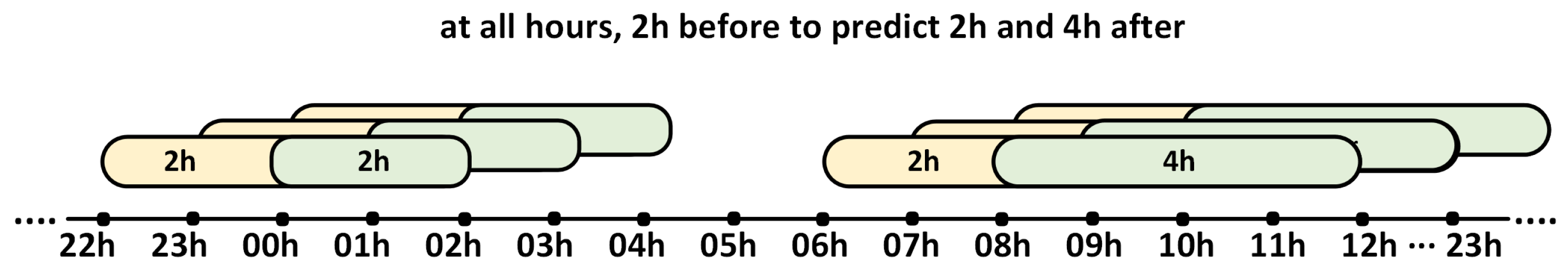
This study presents individualized multiple regression models for each hour of the day aimed at predicting blood glucose (BG) and the CV over extended prediction horizons. The models incorporate a CoDa type regressor (TBR, TIR, TAR), along with other scalar variables that proved valuable in distinguishing when compositional variables exhibited similarities. The dependent variables in the models are the mean and CV of glucose measurements for the next 2 and 4 h.

2. Materials and Methods

2.1. Dataset

The REPLACE-BG dataset, publicly available (NCT02258373) [34], was employed and consists of 226 adult subjects with T1D who underwent CGM for 26 weeks. The study was conducted between May 2015 and March 2016 in adult participants with T1D of more than 1-year duration and with HbA1c of 9.0% (75 mmol/mol) or less. All participants used the Dexcom G4 Platinum CGM system.

Data Preprocessing

The CGM measurements of the patients’ glucose profiles contain gaps in the measurements, thus the data were linearly interpolated when the missing data gap did not exceed 30 consecutive minutes (6 measurements). After interpolating the data, the days with gaps were filtered to obtain valid days. Subsequently, the measurements were organized for the 2 h before and 2 h and 4 h after each hour of the day (00 h, 01 h, 02 h, …, 23 h) (Figure 1). With these measurements already divided into groups of 2 h and 4 h, the times in the different glucose ranges for the 2 h prior to the prediction were calculated, which were treated as three-part CoDa (<70, 70–180, >180) whose sum is constant at 100%.

2.2. CoDa

A compositional vector of D parts, whose sample space is the simplex $S^D$, is defined as a vector in which the only relevant information is contained in the relationships between its components (Equation (1)). One way to simplify the use of compositions is to represent them in closed form, that is, as positive vectors, whose parts add up to a positive constant k (in our case 100%). From any vector, it is possible to obtain a composition X of $S^D$ by conveniently scaling the components so that their sum is equal to constant k. In other words, applying the closure operator defined by Equation (2) [23]:

$$\left\{\begin{array}{cc}{x}_i>0,\hfill & i=1,2,\dots ,D.\hfill \\ \sum _{i=1}^D{x}_i=k\hfill & k=cte.\hfill \end{array}\right.$$

(1)

$$\complement \left(X_1,X_2,\cdots ,X_D\right)=\left(\frac{X_1}{{\sum }_{i=1}^D{X}_i},\frac{X_2}{{\sum }_{i=1}^D{X}_i},\cdots ,\frac{X_D}{{\sum }_{i=1}^D{X}_i}\right).$$

(2)

The importance of the scale invariance principle has been demonstrated where the value of k is not relevant, and it has been observed that its practical implementation requires working with component ratios. Therefore, the analysis of logarithmic ratios was implemented for composition problems. Logarithms of ratios are mathematically more manageable than ratios, which has led to the use of log-ratio functions for obtaining the components [23].

The centered log-ratio function ($clr$) (Equation (3)) is symmetric, where $g\left(x\right)$ is the geometric mean by Equation (4).

$$\begin{array}{cc}\hfill clr\left(x\right)& =\left[cl{r}_{1}x,cl{r}_{2}x,\dots ,cl{r}_{D}x\right]\hfill \\ \hfill & =\left[ln\frac{x_1}{g\left(x\right)},ln\frac{x_2}{g\left(x\right)},\dots ,ln\frac{x_D}{g\left(x\right)}\right].\hfill \end{array}$$

(3)

$$\begin{array}{c}\hfill g\left(x\right)={\left(\prod _{i=1}^D{x}_i\right)}^{\frac{1}{D}}.\end{array}$$

(4)

Let $e_1,e_2,\dots ,e_{D-1}$ be an $olr$-basis in $S^D$, the function that assigns coordinates with respect to $e_1,e_2,\dots ,e_{D-1}$ to a composition $x\in S^D$ is called the isometric transformation log-ratio ilr: $S^D\to {\Re }^{D-1}$ (Equation (5)) [24]. The olr base associated with a sequential binary partition (SBP) can be defined in several ways. The word isometric in $ilr$ refers to the preservation of distance. In [35], the name $olr$ was introduced to avoid confusion because the $clr$ transformation is also an isometric log-ratio transformation.

$$ilr\left(x\right)=[{\langle x,e_1\rangle }_a,\dots ,{\langle x,e_{D-1}\rangle }_a].$$

(5)

The study methodology is described in Figure 2, which includes the analysis of BG measurements, data processing, and implementation of the multiple regression model, whose inputs are the olr-coordinates (olr1(x), olr2(x)) corresponding to the CoDa vector (TBR, TIR, TAR), transformed scalar variables (mean, CV, minimum, and maximum) of the 2 h before and the outputs are the transform of the mean and CV of 2 and 4 h after, model validation, and, finally, the application of “traffic light with symbols” as a decision support system (DSS).

2.3. Regression Model with CoDa

In general, there are three types of linear regression models (LRM) that involve CoDa [23,36,37]. Type I (multivariate model) has a composition as the response and one or more non-compositional (scalar) variables as explanatory [23]. Type II has composition as explanatory and a non-compositional response; if the response is univariate, it is a multiple LRM. Finally, type III has both composition as explanatory and composition as response, becoming a multivariate multiple LRM. For each type, the regression model can be constructed using the Euclidean structure of the simplex or the $olr$ coordinates or transformed $clr$ scores. However, because there are infinite possibilities to construct $olr$ coordinates [24], it is important to focus on those that allow interpretation of the model and the corresponding regression coefficients.

2.3.1. LRM with Compositional Predictor and Scalar Response

Multiple linear regression (MLR) models are a statistical technique widely used to predict a response variable (y) from one or more explanatory variables (x). In the context of an MLR model, the compositional vector x (belonging to the simplex composition space, $S^D$) is used as the explanatory variable of the model to predict the response variable y. In this type of model, no statistical assumptions are made about the composition of x, but only about the residuals u of the response variable y that is being predicted. It is assumed that the residuals are normally distributed and have constant variance. Residual diagnostics are performed in the same way as in a standard MLR and a single equation model is fitted, whose coefficient of determination (${\Re }^2$) is directly interpretable [38].

Steps for the Creation of the Model Based on CoDa

• An $olr$ base is selected in $S^D$ using an SBP (

  Table 1. Sequential binary partition.

  i	${\mathit{X}}_{<70}$	${\mathit{X}}_{70-180}$	${\mathit{X}}_{>180}$	$\mathit{p}(+)$	$\mathit{n}(-)$
  1	+1	+1	−1	2	1
  2	+1	−1	0	1	1

  ) [38].
• The predictor is represented in $olr$-coordinates (Equation (6)). The compositions are, by definition, multivariate and therefore must be mapped in some way, linear or non-linear, to a single number. To compute such a regression model, the principle of working in coordinates is used to transform the model into a multiple regression problem. The $olr$-coordinate $x^{\ast }$, of a composition x with respect to a base linked to a SBP, is calculated as Equation (7).

  $$x_j^{\ast }=olr\left(x\right)\in {\Re }^{D-1}.$$

  (6)

  $$x_j^{\ast }=\sqrt{\frac{p_j\ast n_i}{p_j+n_i}}ln\frac{{(x_{k_1}\dots x_{k_{p_j}})}^{1/p_i}}{{(x_{l_1}\dots x_{l_{n_j}})}^{1/n_i}}$$

  (7)

  where $k_1,\dots ,k_{p_j}$ are the labels of the parts in the numerator (encoded by +1 in the ith row of SBP), $l_1,\dots ,l_{n_j}$ are the labels of the parts in the denominator (encoded by −1 in the same row) and $j:1,\dots ,D-1$.
• The ordinary regression model is solved to obtain the coefficients ${\beta }^{\ast }$ with Equation (8) for $i=1,\dots ,n$.

  $$y_i={\beta }_0+{\beta }_1^{\ast }{x}_{i1}^{\ast }+\dots +{\beta }_{D-1}^{\ast }{x}_{iD-1}^{\ast }+u_i.$$

  (8)

The $ilr$ transformation has been used, as it satisfies the requirement that the analysis has to be permutation invariant. On the other hand, the $clr$ transformation is not easy to interpret with compositional explanatory variables because it produces numerical problems with singular matrices in the tests [26].

2.3.2. Data Preprocessing

The compositional input could contain zeros if some of the parts of the CoDa vector were zero; therefore, a pre-treatment was done because CoDa is based on log-ratios of parts. The detection matrix (dL) used in the imputation of the zeros was interpreted as in [17], taking into account the consecutive zeros. In this case, where we are only analyzing three parts, there could only be two consecutive zeros; the dL value will then be calculated by dividing 5 min (sensor measurement interval) by 120 min, which is the time analyzed from the previous 2 h, dL = 0.04166. We consider that the further zero is from the non-zero value, the smaller this value should be in the dl matrix, as presented in

Table 2. Detection limit matrix for 2 and 4 h.

Consecutive Zeros	Position 1	Position 2
For 2 h, 5/120 = 0.04166
1	dL = 0.04166
2	dL/3 = 0.01388	2 dL/3 = 0.0277
For 4 h, 5/240 = 0.02083
1	dL = 0.02083
2	dL/3 = 0.00694	2 dL/3 = 0.01388

. To make the replacement, we used the multRepl (multiplicative simple replacement) function implemented in the package “zCompositions” of R version 4.1.2; this method provides a compositional counterpart to the common simple substitution by a fixed fraction of the censoring threshold. The remaining components are multiplicatively adjusted to preserve the relative multivariate structure of the data [39,40,41]. The scalar variables have also been transformed (function ln) beforehand to estimate the ordinary regression models (Step 3). This decision is shared by all LRMs because it is an option due to the nature of the covariate (sample space, distribution, etc.). In addition, an outlier analysis could be performed at this step [38].

In this study, 24 multiple LRMs were implemented for each hour of the day. We utilized a compositional input based on the time vector within each BG range, starting from 2 h before, and obtained scalar outputs representing the mean and coefficient of variation (CV) of glucose levels 2 h and 4 h later. Subsequently, a multiclass classifier was implemented (Figure 3), utilizing the predictions of mean and CV, as well as estimates of minimum and maximum glucose levels, to categorize the periods into 3 and 5 classes. Following this, validation was conducted using 80% of the data for training and the remaining 20% for validation. Although it is an individualized model, the results are presented for the entire cohort.

2.4. Prediction of Minimum and Maximum Glucose

CV is calculated according to Equation (9). It is a measure of variability relative to the mean [42]; solving for Equation (10) (glucose standard deviation (STD)) is obtained, knowing the mean and CV previously predicted by the multiple LRM for the next 2 h and 4 h. Under the assumption of normality, it can be said that the minimum and maximum glucose values are in the range of $\pm 3STD$ (99.7∼100%), where $\overline{x}$ is the mean glucose.

$$CV=\frac{STD}{\overline{x}}\ast 100.$$

(9)

$$STD=\frac{CV\ast \overline{x}}{100}.$$

(10)

2.5. Confusion Matrix—Metrics for Multi-Class Classification

In machine learning, “multi-class classification” tasks involve categorizing data into more than two classes [43,44,45]. Performance metrics are valuable for assessing and comparing various classification models or machine learning methods (

Table 3. Metrics for multi-class classification.

Metrics	Equation
Accuracy metric accounts for the correct classifications (TP and TN) and incorrect classifications in the confusion matrix.	$Accuracy=\frac{TP+TN}{TP+TN+FP+FN}$
Balanced Accuracy (BA) calculates the average recall for each true class, considering class imbalances to provide a fair assessment of model performance across all classes.	$\mathrm{BA}=\frac{\frac{AA}{\sum ro{w}_1}+\frac{BB}{\sum ro{w}_2}+\frac{CC}{\sum ro{w}_3}}{tota{l}_{class}}$
BA Weighted (BAW) leverages the BA formula by incorporating class weights, determined by class frequencies in the dataset. This enables the monitoring of algorithm performance for individual classes and highlights the impact of each class based on its frequency.	$\mathrm{BAW}=\frac{\frac{AA}{\sum ro{w}_1}\ast AA+\frac{BB}{\sum ro{w}_2}\ast BB+\frac{CC}{\sum ro{w}_3}\ast CC}{AA+BB+CC}$
Precision	$Precisio{n}_{class}=\frac{T{P}_{class}}{T{P}_{class}+F{P}_{class}}$
Recall	$Recal{l}_{class}=\frac{T{P}_{class}}{T{P}_{class}+F{N}_{class}}$
Macro Average Precision (MaAP)	$\mathrm{MaAP}=\frac{{\sum }_{calss=1}^{clas{s}_{max}}Precisio{n}_{class}}{clas{s}_{max}}$
Macro Average Recall (MaAR)	$\mathrm{MaAR}=\frac{{\sum }_{calss=1}^{clas{s}_{max}}Recal{l}_{class}}{clas{s}_{max}}$
Micro F1-Score	$\mathrm{Micro}\mathrm{F}1-\mathrm{Score}=\frac{{\sum }_{calss=1}^{clas{s}_{max}}T{P}_{class}}{\mathrm{Total}}$
Macro F1- Score	$\mathrm{Macro}\mathrm{F}1-\mathrm{Score}=2\ast \frac{\mathrm{MAP}\ast \mathrm{MAR}}{\mathrm{MAP}+\mathrm{MAR}}$
Macro F1- Score	$\mathrm{Macro}\mathrm{F}1-\mathrm{Score}=2\ast \frac{\mathrm{MAP}\ast \mathrm{MAR}}{\mathrm{MAP}+\mathrm{MAR}}$
Micro Average Precision (MiAP)	$\mathrm{MiAP}=\frac{{\sum }_{calss=1}^{clas{s}_{max}}T{P}_{class}}{\mathrm{total}\mathrm{per}\mathrm{column}}$
Micro Average Recall (MiAR)	$\mathrm{MiAR}=\frac{{\sum }_{calss=1}^{clas{s}_{max}}T{P}_{class}}{\mathrm{total}\mathrm{per}\mathrm{row}}$
Matthews Correlation Coefficient (MCC) where K is the number of classes, $n_{ii}$ is the number of samples correctly classified in class i, and $n_{ij}$ is the number of samples that were classified as i but belong to class j. The numerator of the formula represents the covariance between the predictions and the true labels, whereas the denominator is a normalization to bring the result in the range [−1, 1].	$\mathrm{MCC}=\frac{{\sum }_{i=1}^K{\sum }_{j=1}^K{n}_{ii}{n}_{jj}-{\sum }_{i=1}^K{n}_{ii}{\sum }_{j=1}^K{n}_{ij}}{\sqrt{\left({\sum }_{i=1}^K{n}_{ii}-{\sum }_{i=1}^K{\sum }_{j=1}^K{n}_{ij}\right)\left({\sum }_{i=1}^K{n}_{ii}-{\sum }_{j=1}^K{n}_{ij}\right)}}$

). The confusion matrix, represented in

Table 4. Confusion matrix.

	Predicted Data
	Class	A	B	C
Real Data	A	AA	AB	AC
	B	BA	BB	BC
	C	CA	CB	CC

, quantifies agreements and discrepancies between actual and predicted classifications. It displays classes in a consistent order in both rows and columns, with accurate predictions located on the main diagonal, indicating the frequency of correct predictions.

3. Results

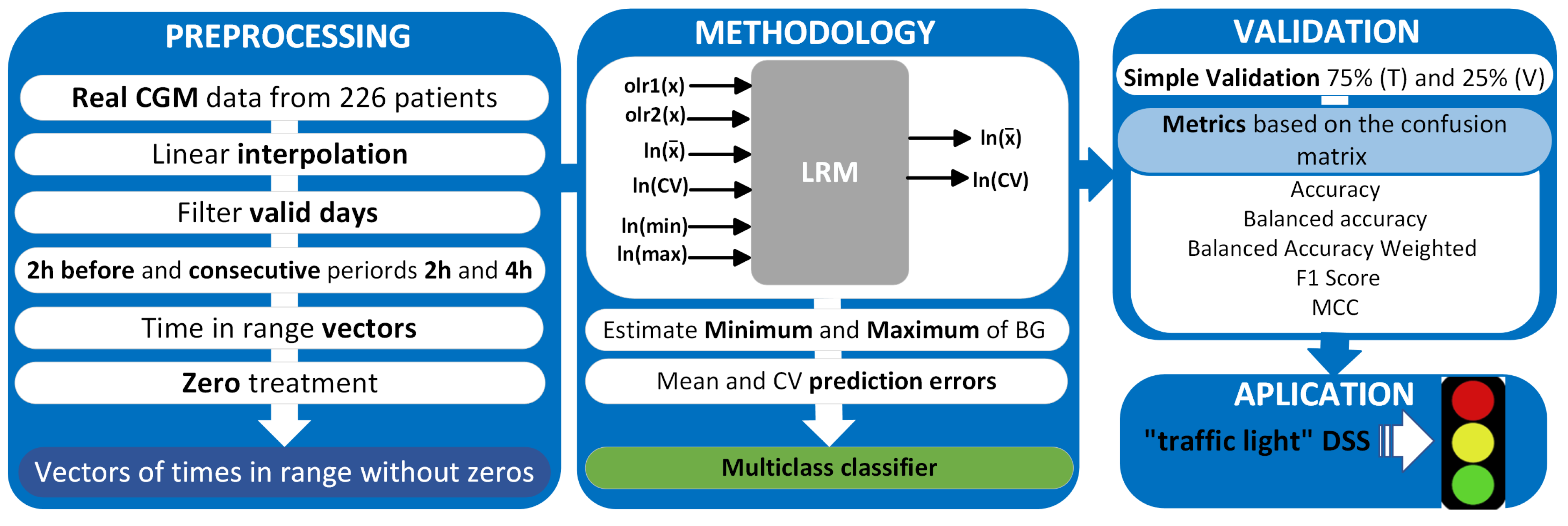
Below are the detailed results for glucose mean and CV prediction as well as metrics for the classification and DSS.

3.1. Overall LRM Test Results

Compared to univariate linear regression, it is not possible to display the strength of the relationship between multiple composition variables (orthogonal basis of different time in ranges of glucose) and a dependent variable (mean, CV) in a single XY scatter plot because X has several potentially influential components [26].

To test the normality assumption of the residuals, the Shapiro–Wilk test was used, which showed a p-value > 0.05, suggesting that we cannot reject the null hypothesis that the data come from a normally distributed population.

Non-constant variance score and Breusch–Pagan tests were performed to verify the homoscedasticity assumption, that is, “all errors have the same variance”. The results showed a p-value > 0.05, suggesting that the homoscedasticity assumption is met. Additionally, the independence assumption of the errors was checked using the Durbin Watson test, and no evidence of violation of this assumption was found (p-value > 0.05).

3.2. Validation of the Multivariable LRM of Mean and CV Prediction

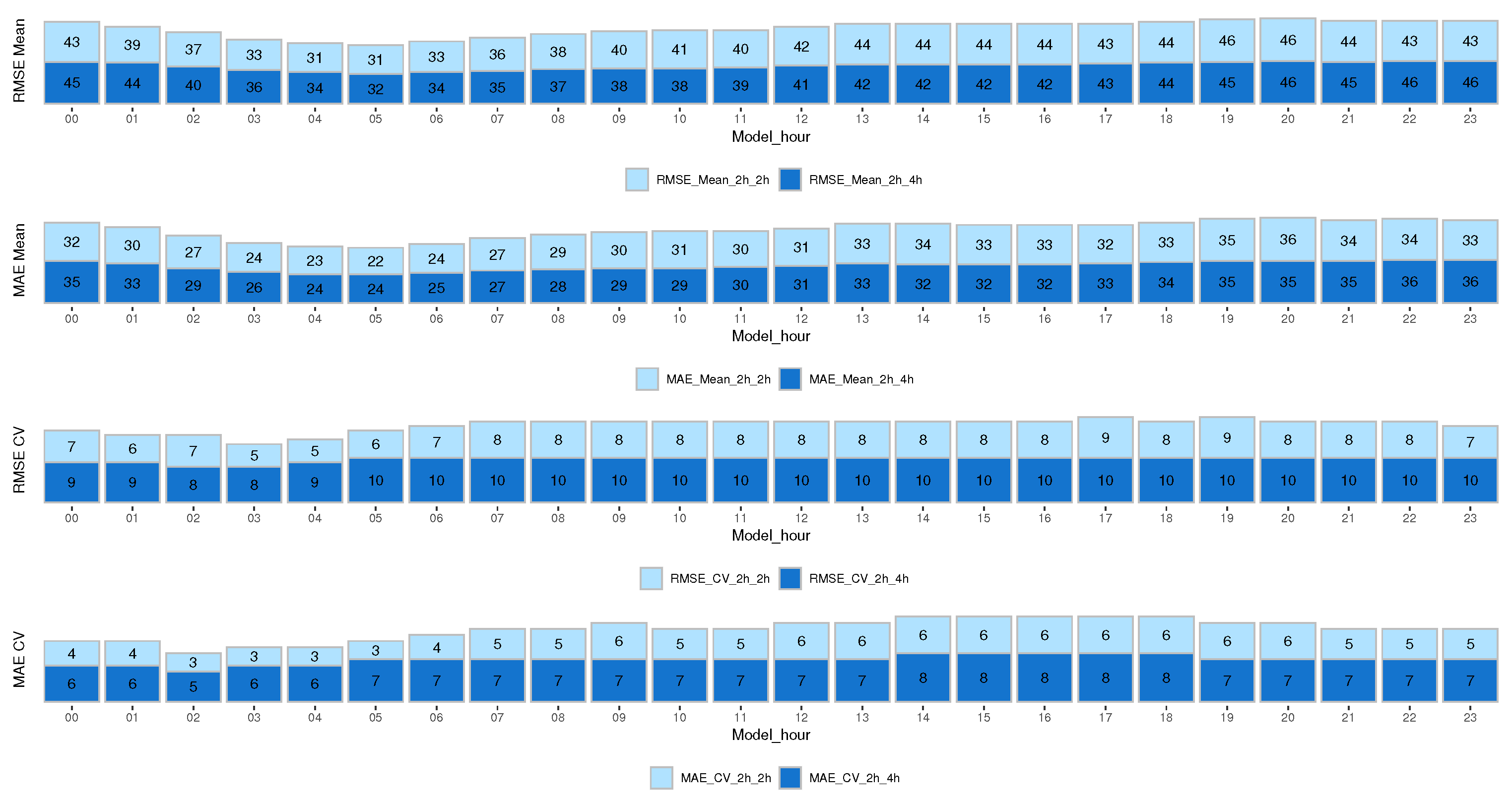
The results are presented in terms of root mean squared error (RMSE) and mean absolute error (MAE) to estimate performance and evaluate the model fit for the entire cohort at different times of the day. Figure 4 shows the results for the mean and CV prediction model for the next 2 h and 4 h. We analyzed both errors since the MAE error is more robust and does not give much importance to outliers, unlike the RMSE, which gives more importance to outliers by squaring the absolute value of the difference. As expected, the RMSE error is higher than the MAE error.

The results show that for the CV prediction, both the RMSE and MAE errors for all models were higher when predicting the next 4 h than when predicting the next 2 h. However, this did not happen with the mean glucose prediction, which remained more uniform.

It is very useful to identify glycemic trends at different times of the day, quantify glycemic variability, and stratify the risk of hypoglycemia based on the hours. In the early morning hours (01:00 to 08:00 h), the RMSE and MAE errors were lower for the mean model compared to the rest of the hours. Similarly, for the CV model, the RMSE error during the hours from 00:00 to 07:00 h was lower than the rest of the hours, and the MAE error was lower from 23:00 to 07:00 h. This shows that our model is capable of predicting early morning hours with higher reliability (lower errors). This factor is significant for both the risk of experiencing nocturnal hypoglycemia and the dawn phenomenon, which typically happens between 04:00 and 08:00 h in the morning.

Also, the distributions between the real and predicted means and CV were compared to detect if there were differences between them. The Kolmogorov–Smirnov statistic was used. The main advantage of this statistic is that it is sensitive to differences in both the location and shape of the cumulative distribution function. The results showed a p-value > 0.05 in all time periods, suggesting that we cannot reject the null hypothesis that the analyzed data follow the same distribution.

3.3. Application, Example of the “Traffic Light” Proposed for a Specific Patient

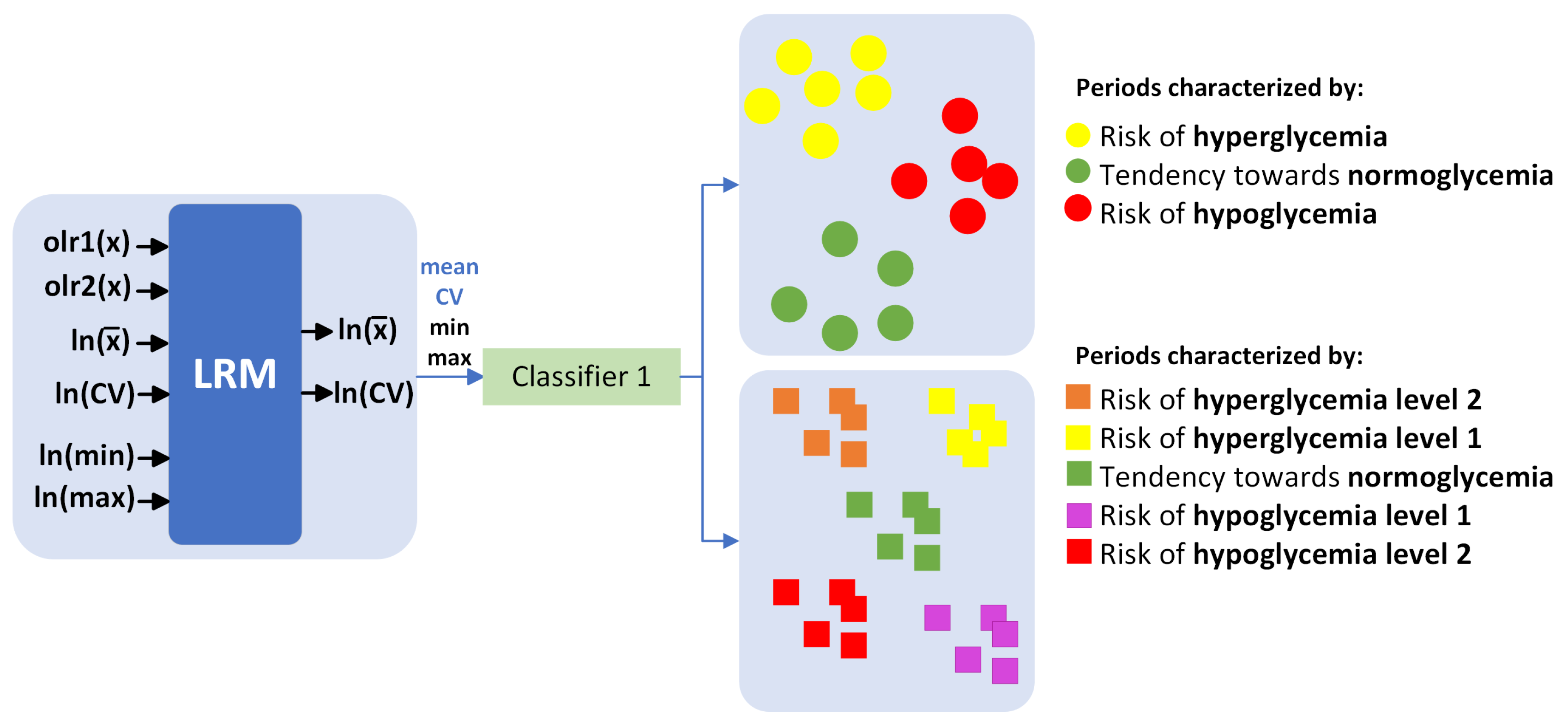
“Traffic light” systems for clinical information and clinical support are well known [46,47]. Using the multiple linear regression model’s predictions for mean and coefficient of variation, in addition to the estimates for minimum and maximum glucose levels over the next 2 and 4 h, a methodology was implemented to categorize each hour of the day into 3 and 5 categories, as illustrated in Figure 3. The categorization criteria were defined based on the standards outlined in [13]. The glucose time in range percentages were as follows: for three categories, $BG<70$ mg/dL, $70\le BG\le 180$ mg/dL, and $BG>180$ mg/dL. The criteria for the five categories were more stringent: $BG<54$ mg/dL, $54\le BG<70$ mg/dL, $70\le BG\le 180$ mg/dL, $180<BG\le 250$ mg/dL, and $>250$ mg/dL. This system provides qualitative information about the future glucose state based on these estimates.

Patient 1, Day 3 Characterized by High Variability

Table 5. Example of “traffic light” for patient 1, day 3, with 3 and 5 class to predict the next 2 h.

	3 Class		5 Class
Hour	Predicted State	Real State	Predicted State	Real State	Characteristics of the States
00:00					3 class
01:00
02:00
03:00
04:00
05:00
06:00
07:00					5 class
08:00
09:00
10:00
11:00
12:00
13:00
14:00
15:00
16:00
17:00
18:00
19:00
20:00
21:00
22:00
23:00

presents an example of the proposed “traffic light” system for patient 1. We have analyzed day 3, as it is a day with high glucose variability (36.53%), severe hyperglycemia both during the day and at night, and also the presence of hypoglycemia. Column 4 shows the description for each of the previously mentioned classes. Analyzing the predictions of the states for 3 class (column 2 of Table 5), it can be seen that from 00:00 to 18:00 h, for every hour in that interval, the model predicted that the patient would be there for the next 2 h in hyperglycemia (>180 mg/dL); the actual states validate that the model was correct every time. During the night period, from 22:00 h of the previous day to 8:00 h, this patient experienced a glucose variability of 6.5%, with a minimum reading of 269 mg/dL and a maximum of 371 mg/dL, indicating severe hyperglycemia.

From 19:00 to 20:00 h, he was in the target glucose range (70–180 mg/dL), a situation that the model also correctly predicted. However, from 21:00 to 23:00 h, the patient was in hypoglycemia, a situation predicted by the model.

Still considering the prediction of 2 h, by analyzing the results for 5 class, from 00:00 to 17:00 h, the model predicted severe hyperglycemia, being more specific than when it was analyzed for 3 class. It was found that the minimum glucose was 244 mg/dL and the maximum was 329 mg/dL, and the CV for 2 h was between 2% and 8%. However, at 18:00 h, the model predicted risk of hyperglycemia; here we verified that the patient had a minimum of 70 mg/dL and a maximum of 321 mg/dL with a CV of glucose for the next 2 h of 40%, and vector time in range was 0% below 70 mg/dL, and 50% for both TIR and hyperglycemia above 180 mg/dL, that is, half of the next 2 h was spent time in normoglycemia and the rest in hyperglycemia.

Hence, at 19:00 and 20:00 h, the patient will behave in range time. At 21:00 and 22:00 h, the model predicted risk of hypoglycemia; however, the validation corroborated that it was accurate for 21:00 h, but for 22:00 h, the real state reported severe hypoglycemia. The time vector in range glucose reported 66% of time below 70 mg/dL, 33.3% in TIR, and 0% above 180 mg/dL. For 23:00 h, both the model and reality reported severe hypoglycemia. In practice, as we have shown in this example, it is expected that the patient will have the 24 models for each hour of the day, and the prediction model will update him on his future status for the next 2 h.

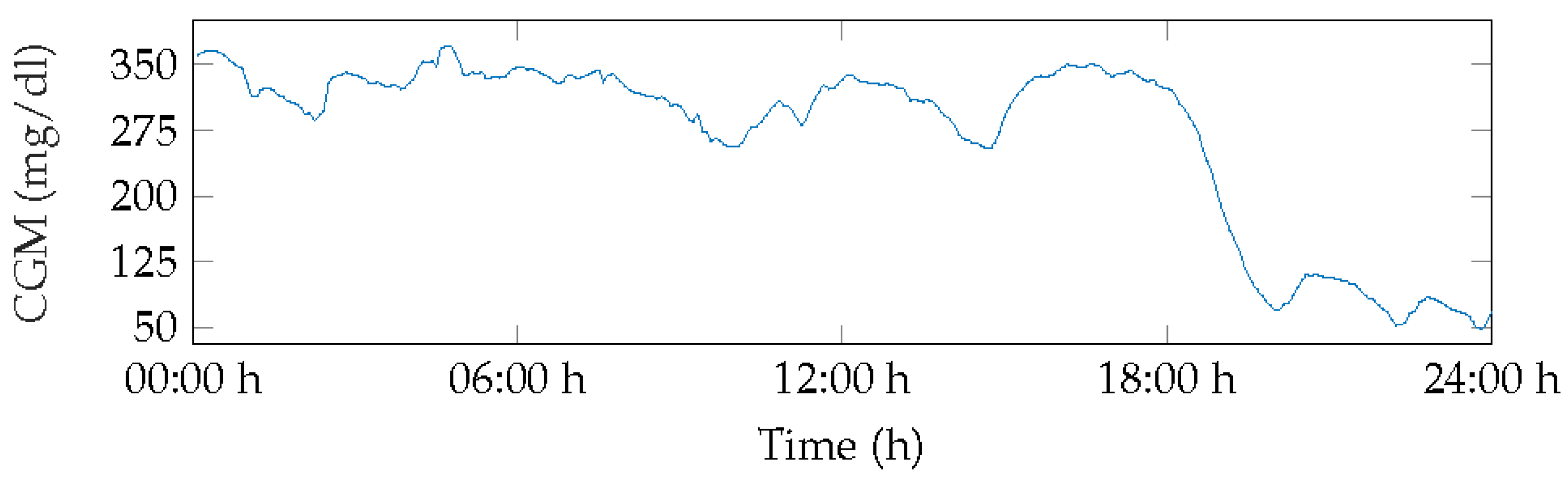
Figure 5 displays the BG measurements for Patient 1 for day 3. This day showed severe hyperglycemia for over 50% of the time, with the first minimum peak at 70 mg/dL occurring at 20:00 h, increasing glucose levels, and levels remaining in range until 22:00 h before dropping to hypoglycemia level 1 with few normoglycemic measurements.

3.4. Results of the Metrics for Multi-Class Classification

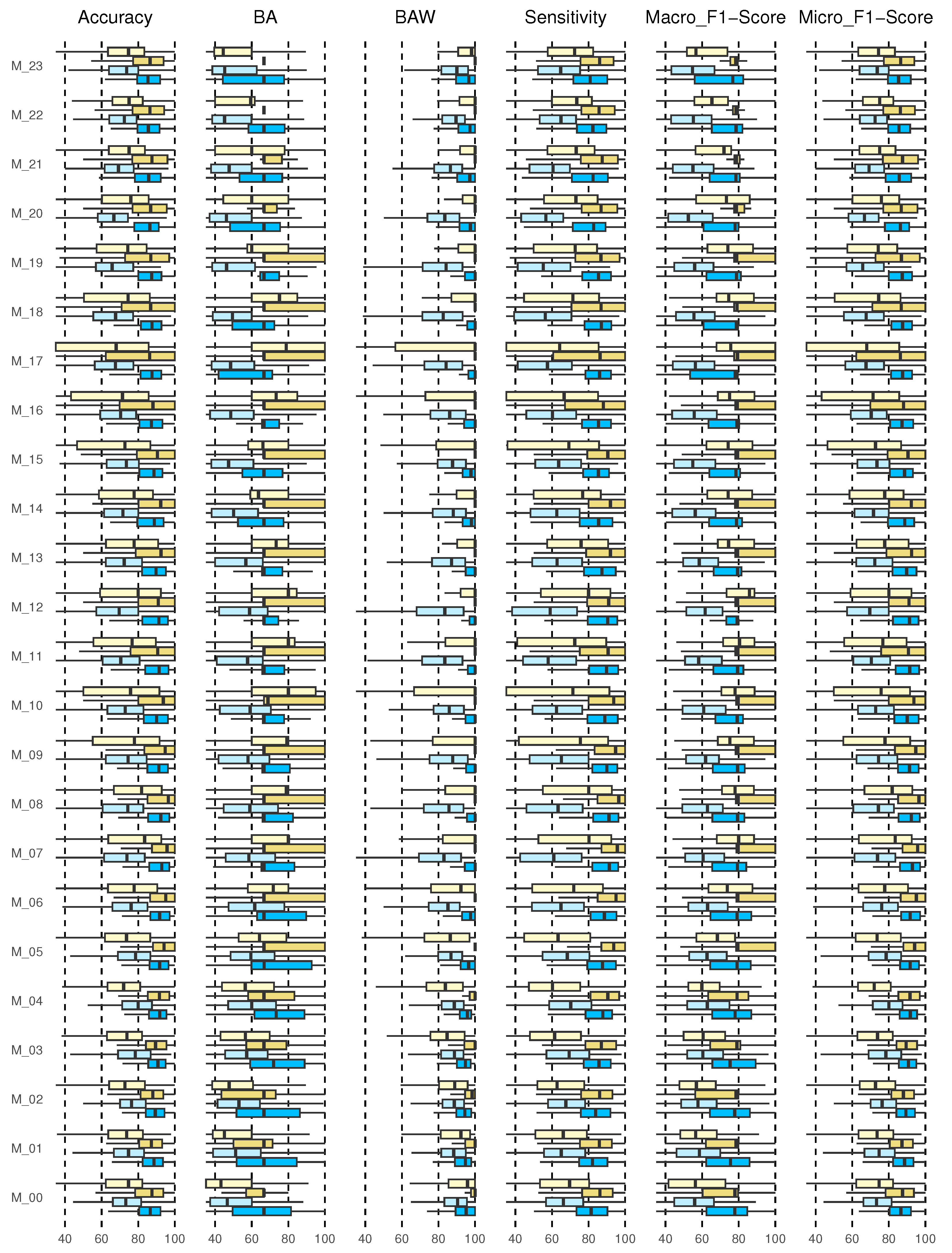
Once the actual and predicted data from the validation data were classified, the confusion matrix was created for each of the 24 models and each of the 226 patients. Although this is an individualized model, the metrics results are shown for the entire cohort. Figure 6 shows the results for accuracy, BA, BAW, sensitivity, and macro and micro F1-scores. Each of the results will be discussed below.

3.4.1. Accuracy Results

The accuracy returns a general measure of how correctly the model predicts for all samples. The results for the entire cohort are shown in the boxplot in Figure 6 (first graph on the left).

The diagrams show the results of the predictions of the 24 models (M_00, M_01, …, M_23) corresponding to each hour of the day. The prediction of 2 h and 4 h with 3 and 5 classes are shown. This type of graph allows us to identify outliers and compare distributions, as well as knowing in a comfortable and fast way how 50% of the central values are distributed. The dimensions of the boxes are determined by the distance of the 25th–75th interquartile ranges. At all times, these distances were greater when the prediction horizon (PH) was longer (4 h), and they increased for the 5-class categorization.

For the prediction of 2 h, 3 and 5 classes, it is evident that the median is located in the center of the box, then the distribution is symmetric and the mean, median, and mode coincide, except for 2 h 3 class (M_04, M_07, M_11, M_14, M_20) and for 2 h, 5 class (M_07, M_08). For the prediction of 4 h, 3 class for schedules M_00 and M_06 to M_18, negative asymmetry is shown, as the longest part is the lower part of the median. Therefore, the data were concentrated in the upper part of the distribution. Here, the mean is usually less than the median; this shows dispersion in the data, not a greater value. For the prediction of 2 h and 4 h for 3 classes at all times, an accuracy greater than 85% was reached at all times of the day with a 75th quartile close to 100%. For 5 classes, the 4 h forecast presented better performance, although the data were more dispersed, with a 75th close to 90% for all times.

3.4.2. Balanced Accuracy and Balanced Accuracy Weighted Results

Figure 6 shows the results of the BA and BAW (second and third graph, respectively, from left to right). The results of the BA for 2 h, 3 classes for schedules M_00 to M_05 and M_15 behave symmetrically; however, the model for schedules M_13, M_17, M_20, M_21, and M_23 show negative asymmetry. For the 4 h forecast, except for the hours M_00 to M_02, there was positive asymmetry. For M_22 and M_23, all the results were concentrated in the median. At all times, the 75th quartile was above 70%. For the prediction to 5 classes, symmetry was observed only for 2 h in M_03, M_04, and M_07 to M_10. For the rest, there was generally positive asymmetry. Here, the 75th quartile was above 60%; however, it improved for the 4 h forecast, exceeding 80%. The results for 3 classes are satisfactory, although no symmetric distribution was observed in the results for any model. In all cases, the median was greater than 90% and the 75th quartile close to 100%. For the prediction with 5 classes, the results were observed to be more dispersed, especially in the hours from M_08 to M_10, M_16, and M_17. Symmetry was not observed.

3.4.3. Sensitivity Results

The results show that, for the prediction with 3 classes, the median was above 80% in all cases, with the 75th quartile close to 100%. However, the cohort data were more dispersed when 5 classes were evaluated, finding the median close to 75% for all hours and with a greater dispersion in daytime hours from M_05 to M_20 (Figure 6 (fourth graph from left to right)).

3.4.4. F1-Score

In this study for the prediction with 3 classes, the results of the median for the entire model for the prediction at both 2 h and 4 h was higher than 80%, with a 75th quartile close to 100%, thus, the same in the hours from M_05 to M_19, indicating that the algorithm performs well in all classes. However, for 5 classes, the median for 2 h in all cases was above 60% but for 4 h in some cases above 70% (M_06 to M_21).

Micro-average considers all units together, without taking into account possible differences between classes, just like accuracy. Both measures give more importance to large classes, because they only consider all units together. In our case, all classes are important, so we should not underestimate the small ones. In addition, at some times the large classes for our model are usually TIR, which, although they provide information, do not suggest any corrective action. Even so, the results showed a median higher than 8% and 75% for when there are 3 classes and 5 classes, respectively. Very scattered results were not observed in any case, although there was a difference between the prediction with 3 and 5 classes.

3.4.5. Matthews Correlation Coefficient for Multi-Class Classification

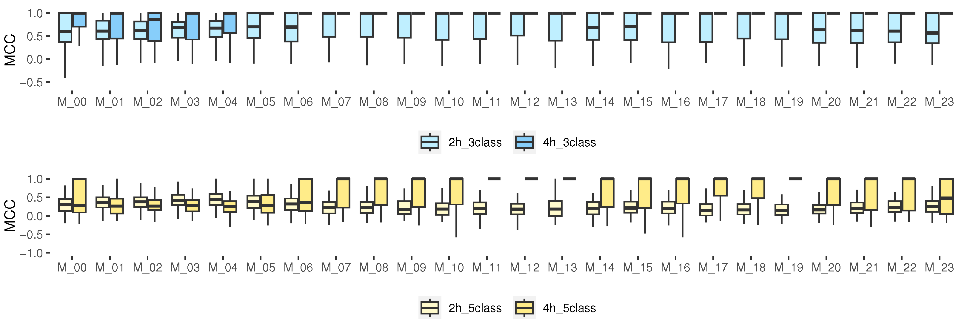
Among the advantages of this metric, we can see that MCC includes all the entries of the confusion matrix in both the numerator and the denominator [48,49]. Our results (Figure 7) show that, for the prediction with 3 classes, especially for 4 h, the median for the hours from M_05 to M_23 was 1, indicating a perfect prediction. However, for 5 classes, such a median was only obtained for the models from M_07 to M_22 for 4 h. The rest of the hours, the median was close to 0.5 (greater than 0.5 is considered good). For some isolated cases, it was close to 0, which corresponds to a random prediction of the model, and some very isolated samples were below zero, which indicated a totally incorrect prediction. For 3 classes, it could be considered as an accurate model; however, for some schedules of 5 classes, it indicates that the model is not better than a random prediction.

4. Discussion

DSSs have proven to be useful tools for patients and physicians [2,46,47]. Although glucose profiles have been treated as CoDa vectors in previous studies [15,16,17], there is no application in this branch of mathematics that is focused on predicting the mean and the CV as an information system or DSS tool for patients with T1D at specific hours of the day oriented to wide PH (2 h and 4 h). In this work, CoDa variables and transformed scalars have been used to predict the mean and CV of glucose in patients with T1D. In addition, the different times of the day of the patients have been categorized to provide an idea of the behavior of glucose in the next 2 h and 4 h. The results have been validated using a sample of 226 adult patients from a real cohort.

Although no study was found that predicted the mean and CV for patients with T1D at a PH of 120 and 240 min, prior research has focused on glucose prediction within time horizons ranging from 15 to 120 min [3,4,5,6,7,8]. As expected, the longer the forecast horizon, the greater the error. Specifically, for a 120 min PH, errors typically exceed 45 mg/dL, as reported in previous studies [5,6,8,50].

The results show that the MAE mean prediction error is between 23 and 36 mg/dL for all times, when predicting at both 2 h and 4 h. The CV is between 4 and 7% for the 2 h prediction and between 6 and 8% for the 4 h prediction. The RMSE and MAE prediction error of the mean and CV at all times of the day was higher for the 4 h forecast horizon in the entire cohort, but the early morning times presented a lower error. It was confirmed that the CV at this time was lower than during the daytime hours.

Previous studies have used some of these metrics based on the confusion matrix to evaluate the performance of different methodologies [48,49]. In [48], population outcomes for the mid-term continuous prediction module to predict hypoglycemia and population outcomes for the nocturnal hypoglycemic events predictor module are reported, with average mean of accuracy of 86.1% and 80.1%, respectively. Also, mean sensitivity of 48.5% and 44%, respectively, was reported. Here, there was a mean MCC of 0.51 with a minimum of −0.18 and a maximum of 0.86 for the mid-term continuous prediction module to predict hypoglycemia. In [49], a cohort of 10 real patients was studied using support vector machines. The researchers presented the results, which evaluated the model’s performance with and without including physical activity measures. The findings showed that the median sensitivity for both scenarios was 71% and 70%, respectively. Furthermore, analyzing individual patients revealed that the median F1-scores ranged from 37% (patient 12) to 80% (patient 45), indicating varying levels of accuracy. Remarkably, excluding physical activity measures did not result in significant changes in this metric. Additionally, the reported MCC varied from 0.2 (patient 12) to 0.67 (patient 56).

The DSS provided interesting results in different metrics, such as accuracy, BA, BAW, sensitivity, F1-score, and MCC. They were higher than 90% for the entire cohort for 3 classes, but for 5 classes they decreased, obtaining results above 80%. Therefore, the system will be more reliable and accurate when 3 classes are used according to some metrics.

It should be noted that the results for the 4 h prediction, both for the 3 and 5 class scenarios, exhibited greater dispersion, which underscores the variability within the cohort; nevertheless, they yielded satisfactory outcomes. The outcomes presented in this article pertain to the entire cohort; however, it is an individualized model, and it is important to acknowledge that some patients achieved better results than others. Therefore, the results are presented in a median and interquartile range format. The prediction results were all below 45 mg/dL for every time frame. Furthermore, a model is proposed for each hour of the day, taking into account daytime, nighttime, and postprandial time frames, which are of particular interest due to the impact of day-to-day variability. We predict not only the mean but also the CV, as within a specific time range, the mean can remain the same while the CV varies. This could pose significant risks in patients with type 1 diabetes. Additionally, predictions have been made for extended prediction horizons (2 and 4 h), which are often challenging to achieve good results. The authors anticipate that this model should be updated and adjusted over time, considering the habits and characteristics of individual patients.

5. Conclusions

In this study, we presented a methodology for multiple regression models based on CoDa to predict glucose outcomes over long time horizons (2 h and 4 h). The model has been created and validated using a substantial dataset of real patients. Good results have been obtained from both the regression models and the proposed DSS, indicating the reliability of the proposal. The novelty of this work lies in the long-term prediction at each hour of the day for type 1 diabetes patients using a compositional approach.

References

1. Silva, J.A.d.; Souza, E.C.F.d.; Echazú Böschemeier, A.G.; Costa, C.C.M.d.; Bezerra, H.S.; Feitosa, E.E.L.C. Diagnosis of diabetes mellitus and living with a chronic condition: Participatory study. BMC Public Health 2018, 18, 699. [Google Scholar] [CrossRef] [PubMed]
2. Contreras, I.; Vehi, J. Artificial intelligence for diabetes management and decision support: Literature review. J. Med Internet Res. 2018, 20, e10775. [Google Scholar] [CrossRef] [PubMed]
3. Mohebbi, A.; Johansen, A.R.; Hansen, N.; Christensen, P.E.; Tarp, J.M.; Jensen, M.L.; Bengtsson, H.; Mørup, M. Short term blood glucose prediction based on continuous glucose monitoring data. In Proceedings of the 2020 42nd Annual International Conference of the IEEE Engineering in Medicine & Biology Society (EMBC), Montreal, QC, Canada, 20–24 July 2020; pp. 5140–5145. [Google Scholar]
4. Martinsson, J.; Schliep, A.; Eliasson, B.; Mogren, O. Blood glucose prediction with variance estimation using recurrent neural networks. J. Healthc. Inform. Res. 2020, 4, 1–18. [Google Scholar] [CrossRef] [PubMed]
5. Daniels, J.; Herrero, P.; Georgiou, P. A multitask learning approach to personalized blood glucose prediction. IEEE J. Biomed. Health Inform. 2021, 26, 436–445. [Google Scholar] [CrossRef] [PubMed]
6. Tena, F.; Garnica, O.; Lanchares, J.; Hidalgo, J.I. Ensemble Models of Cutting-Edge Deep Neural Networks for Blood Glucose Prediction in Patients with Diabetes. Sensors 2021, 21, 7090. [Google Scholar] [CrossRef]
7. Cichosz, S.L.; Kronborg, T.; Jensen, M.H.; Hejlesen, O. Penalty weighted glucose prediction models could lead to better clinically usage. Comput. Biol. Med. 2021, 138, 104865. [Google Scholar] [CrossRef]
8. Wadghiri, M.; Idri, A.; El Idrissi, T.; Hakkoum, H. Ensemble blood glucose prediction in diabetes mellitus: A review. Comput. Biol. Med. 2022, 147, 105674. [Google Scholar] [CrossRef]
9. Woldaregay, A.Z.; Årsand, E.; Walderhaug, S.; Albers, D.; Mamykina, L.; Botsis, T.; Hartvigsen, G. Data-driven modeling and prediction of blood glucose dynamics: Machine learning applications in type 1 diabetes. Artif. Intell. Med. 2019, 98, 109–134. [Google Scholar] [CrossRef]
10. Sun, X.; Rashid, M.; Askari, M.R.; Cinar, A. Latent Variables Model Based MPC for People with Type 1 Diabetes. IFAC-PapersOnLine 2021, 54, 294–299. [Google Scholar] [CrossRef]
11. Henao-Carrillo, D.C.; Muñoz, O.M.; Gómez, A.M.; Rondón, M.; Colón, C.; Chica, L.; Rubio, C.; León-Vargas, F.; Calvachi, M.A.; Perea, A.M. Reduction of glycemic variability with Degludec insulin in patients with unstable diabetes. J. Clin. Transl. Endocrinol. 2018, 12, 8–12. [Google Scholar] [CrossRef]
12. Kovatchev, B. Glycemic variability: Risk factors, assessment, and control. J. Diabetes Sci. Technol. 2019, 13, 627–635. [Google Scholar] [CrossRef] [PubMed]
13. ElSayed, N.A.; Aleppo, G.; Aroda, V.R.; Bannuru, R.R.; Brown, F.M.; Bruemmer, D.; Collins, B.S.; Hilliard, M.E.; Isaacs, D.; Johnson, E.L.; et al. 6. Glycemic Targets: Standards of Care in Diabetes 2023. Diabetes Care 2022, 46, S97–S110. [Google Scholar] [CrossRef] [PubMed]
14. ElSayed, N.A.; Aleppo, G.; Aroda, V.R.; Bannuru, R.R.; Brown, F.M.; Bruemmer, D.; Collins, B.S.; Cusi, K.; Das, S.R.; Gibbons, C.H.; et al. Introduction and Methodology: Standards of Care in Diabetes 2023; American Diabetes Association: Arlington, VA, USA, 2023. [Google Scholar]
15. Biagi, L.; Bertachi, A.; Giménez, M.; Conget, I.; Bondia, J.; Martín-Fernández, J.A.; Vehí, J. Individual categorisation of glucose profiles using compositional data analysis. Stat. Methods Med Res. 2019, 28, 3550–3567. [Google Scholar] [CrossRef] [PubMed]
16. Biagi, L.; Bertachi, A.; Giménez, M.; Conget, I.; Bondia, J.; Martín-Fernández, J.A.; Vehí, J. Probabilistic Model of Transition between Categories of Glucose Profiles in Patients with Type 1 Diabetes Using a Compositional Data Analysis Approach. Sensors 2021, 21, 3593. [Google Scholar] [CrossRef] [PubMed]
17. Cabrera, A.; Biagi, L.; Beneyto, A.; Estremera, E.; Contreras, I.; Giménez, M.; Conget, I.; Bondia, J.; Martín-Fernández, J.A.; Vehí, J. Validation of a Probabilistic Prediction Model for Patients with Type 1 Diabetes Using Compositional Data Analysis. Mathematics 2023, 11, 1241. [Google Scholar] [CrossRef]
18. Vigersky, R.A.; McMahon, C. The relationship of hemoglobin A1C to time-in-range in patients with diabetes. Diabetes Technol. Ther. 2019, 21, 81–85. [Google Scholar] [CrossRef]
19. Vettoretti, M.; Cappon, G.; Facchinetti, A.; Sparacino, G. Advanced diabetes management using artificial intelligence and continuous glucose monitoring sensors. Sensors 2020, 20, 3870. [Google Scholar] [CrossRef]
20. Noaro, G.; Cappon, G.; Vettoretti, M.; Sparacino, G.; Del Favero, S.; Facchinetti, A. Machine-learning based model to improve insulin bolus calculation in type 1 diabetes therapy. IEEE Trans. Biomed. Eng. 2020, 68, 247–255. [Google Scholar] [CrossRef]
21. Khanam, J.J.; Foo, S.Y. A comparison of machine learning algorithms for diabetes prediction. ICT Express 2021, 7, 432–439. [Google Scholar] [CrossRef]
22. Makroum, M.A.; Adda, M.; Bouzouane, A.; Ibrahim, H. Machine learning and smart devices for diabetes management: Systematic review. Sensors 2022, 22, 1843. [Google Scholar] [CrossRef]
23. Aitchison, J. The statistical analysis of compositional data. J. R. Stat. Soc. Ser. B 1982, 44, 139–160. [Google Scholar] [CrossRef]
24. Egozcue, J.J.; Pawlowsky-Glahn, V.; Mateu-Figueras, G.; Barcelo-Vidal, C. Isometric logratio transformations for compositional data analysis. Math. Geol. 2003, 35, 279–300. [Google Scholar] [CrossRef]
25. Egozcue, J.J.; Daunis-I-Estadella, J.; Pawlowsky-Glahn, V.; Hron, K.; Filzmoser, P. Simplicial Regression. The Normal Model. J. Appl. Probab. Stat. 2012, 6, 87–108. [Google Scholar]
26. Van den Boogaart, K.G.; Tolosana-Delgado, R. Analyzing Compositional Data with R; Springer: Berlin/Heidelberg, Germany, 2013; Volume 122. [Google Scholar]
27. Pawlowsky-Glahn, V.; Egozcue, J.J.; Tolosana-Delgado, R. Modeling and Analysis of Compositional Data; John Wiley & Sons: Hoboken, NJ, USA, 2015. [Google Scholar]
28. Thió i Fernández de Henestrosa, S.; Martín Fernández, J.A. Proceedings of the 6th International Workshop on Compositional Data Analysis: Girona, Spain, 1–7 de juny de 2015; Departament d’Informàtica, Matemàtica Aplicada, Universitat de Girona: Girona, Spain, 2015. [Google Scholar]
29. Fišerová, E.; Donevska, S.; Hron, K.; Bábek, O.; Vaňkátová, K. Practical aspects of log-ratio coordinate representations in regression with compositional response. Meas. Sci. Rev. 2016, 16, 235–243. [Google Scholar] [CrossRef]
30. Ståhl, F.; Johansson, R. Diabetes mellitus modeling and short-term prediction based on blood glucose measurements. Math. Biosci. 2009, 217, 101–117. [Google Scholar] [CrossRef]
31. Mhaskar, H.N.; Pereverzyev, S.V.; Van der Walt, M.D. A deep learning approach to diabetic blood glucose prediction. Front. Appl. Math. Stat. 2017, 3, 14. [Google Scholar] [CrossRef]
32. Rodríguez-Rodríguez, I.; Chatzigiannakis, I.; Rodríguez, J.V.; Maranghi, M.; Gentili, M.; Zamora-Izquierdo, M.Á. Utility of big data in predicting short-term blood glucose levels in type 1 diabetes mellitus through machine learning techniques. Sensors 2019, 19, 4482. [Google Scholar] [CrossRef]
33. Katsarou, D.N.; Georga, E.I.; Christou, M.; Tigas, S.; Papaloukas, C.; Fotiadis, D.I. Short Term Glucose Prediction in Patients with Type 1 Diabetes Mellitus. In Proceedings of the 2022 44th Annual International Conference of the IEEE Engineering in Medicine & Biology Society (EMBC), Glasgow, Scotland, 11–15 July 2022; pp. 329–332. [Google Scholar]
34. Aleppo, G.; Ruedy, K.J.; Riddlesworth, T.D.; Kruger, D.F.; Peters, A.L.; Hirsch, I.; Bergenstal, R.M.; Toschi, E.; Ahmann, A.J.; Shah, V.N.; et al. REPLACE-BG: A randomized trial comparing continuous glucose monitoring with and without routine blood glucose monitoring in adults with well-controlled type 1 diabetes. Diabetes Care 2017, 40, 538–545. [Google Scholar] [CrossRef]
35. Martín-Fernández, J.A. Comments on: Compositional data: The sample space and its structure. Test 2019, 28, 653–657. [Google Scholar] [CrossRef]
36. Hron, K.; Filzmoser, P.; Thompson, K. Linear regression with compositional explanatory variables. J. Appl. Stat. 2012, 39, 1115–1128. [Google Scholar] [CrossRef]
37. Navarro-Lopez, C.; Linares-Mustaros, S.; Mulet-Forteza, C. The Statistical Analysis of Compositional Data by John Aitchison (1986): A Bibliometric Overview. SAGE Open 2022, 12, 21582440221093366. [Google Scholar] [CrossRef]
38. Coenders, G.; Pawlowsky-Glahn, V. On interpretations of tests and effect sizes in regression models with a compositional predictor. SORT-Stat. Oper. Res. Trans. 2020, 44, 201–220. [Google Scholar]
39. Martín-Fernández, J.A.; Barceló-Vidal, C.; Pawlowsky-Glahn, V. Dealing with zeros and missing values in compositional data sets using nonparametric imputation. Math. Geol. 2003, 35, 253–278. [Google Scholar] [CrossRef]
40. Palarea-Albaladejo, J.; Martín-Fernández, J.A. zCompositions R package for multivariate imputation of left-censored data under a compositional approach. Chemom. Intell. Lab. Syst. 2015, 143, 85–96. [Google Scholar] [CrossRef]
41. Martín-Fernández, J.A.; Hron, K.; Templ, M.; Filzmoser, P.; Palarea-Albaladejo, J. Bayesian-multiplicative treatment of count zeros in compositional data sets. Stat. Model. 2015, 15, 134–158. [Google Scholar] [CrossRef]
42. Gulhar, M.; Kibria, B.G.; Albatineh, A.N.; Ahmed, N.U. A comparison of some confidence intervals for estimating the population coefficient of variation: A simulation study. SORT-Stat. Oper. Res. Trans. 2012, 36, 45–68. [Google Scholar]
43. Rácz, A.; Bajusz, D.; Héberger, K. Multi-level comparison of machine learning classifiers and their performance metrics. Molecules 2019, 24, 2811. [Google Scholar] [CrossRef]
44. Grandini, M.; Bagli, E.; Visani, G. Metrics for multi-class classification: An overview. arXiv 2020, arXiv:2008.05756. [Google Scholar]
45. Tharwat, A. Classification assessment methods. Appl. Comput. Inform. 2021, 17, 168–192. [Google Scholar] [CrossRef]
46. Evans, M.; Morgan, A.R.; Patel, D.; Dhatariya, K.; Greenwood, S.; Newland-Jones, P.; Hicks, D.; Yousef, Z.; Moore, J.; Kelly, B.; et al. Risk prediction of the diabetes missing million: Identifying individuals at high risk of diabetes and related complications. Diabetes Ther. 2021, 12, 87–105. [Google Scholar] [CrossRef]
47. Garden, G.L.; Frier, B.M.; Hine, J.L.; Hutchison, E.J.; Mitchell, S.J.; Shaw, K.M.; Heller, S.R.; Koehler, G.; Hofmann, V.; Gaffney, T.P.; et al. Blood glucose monitoring by insulin-treated pilots of commercial and private aircraft: An analysis of out-of-range values. Diabetes Obes. Metab. 2021, 23, 2303–2310. [Google Scholar] [CrossRef] [PubMed]
48. Vehí, J.; Contreras, I.; Oviedo, S.; Biagi, L.; Bertachi, A. Prediction and prevention of hypoglycaemic events in type-1 diabetic patients using machine learning. Health Inform. J. 2020, 26, 703–718. [Google Scholar] [CrossRef] [PubMed]
49. Parcerisas, A.; Contreras, I.; Delecourt, A.; Bertachi, A.; Beneyto, A.; Conget, I.; Viñals, C.; Giménez, M.; Vehi, J. A machine learning approach to minimize nocturnal hypoglycemic events in type 1 diabetic patients under multiple doses of insulin. Sensors 2022, 22, 1665. [Google Scholar] [CrossRef] [PubMed]
50. De Bois, M.; Ammi, M.; El Yacoubi, M.A. Model fusion to enhance the clinical acceptability of long-term glucose predictions. In Proceedings of the 2019 IEEE 19th International Conference on Bioinformatics and Bioengineering (BIBE), Athens, Greece, 28–30 October 2019; pp. 258–264. [Google Scholar]
Figure 1. The distribution of 2 h periods prior to the prediction (yellow) and the following 2 h and 4 h periods (green). The 2 h period preceding the prediction was treated as a three-part CoDa.
Mathematics 11 04517 g001
Figure 2. Methodology for data analysis, validation, and application.
Mathematics 11 04517 g002
Figure 3. Multiclass classifier.
Mathematics 11 04517 g003
Figure 4. RMSE and MAE results from the mean and CV prediction model for the next 2 h and 4 h.
Mathematics 11 04517 g004
Figure 5. BG of patient 1, day 3.
Mathematics 11 04517 g005
Figure 6. Results for multi-class classification, 2h_3classes, 2h_5classes, 4h_3classes, and 4h_5classes (from the bottom up, from dark blue, light blue, dark yellow, light yellow).
Mathematics 11 04517 g006
Figure 7. MCC results for multiclass classification, 2 and 4 h prediction.
Mathematics 11 04517 g007