An Inventory Model for Growing Items When the Demand Is Price Sensitive with Imperfect Quality, Inspection Errors, Carbon Emissions, and Planned Backorders

Abstract

Inventory models that consider environmental and quality concerns have received some attention in the literature, yet no model developed to date has investigated these features in combination with growing items. Therefore, there is a need to incorporate these three relevant aspects together in a single inventory model to support decisions, compare results, and obtain new knowledge for the complexities of the real world. Moreover, current sustainable inventory management practices aim at mitigating the ecological consequences of an industry while preserving its profitability. The present study aligns with this perspective and introduces an economic order quantity (EOQ) model that considers imperfect quality while also accounting for sustainability principles. More specifically, the model addresses growing items, which have a demand dependent on selling price and the unique ability to grow while being stored in inventory. Additionally, the analysis acknowledges the possibility of classification errors during the inspection process, encompassing both Type-I and Type-II inspection errors. Furthermore, the model permits shortages and ensures that any shortage is completely fulfilled through backorders. The optimization model produces an optimal solution for the proposed model that is derived by optimizing three decision variables: order quantity of newborn items, backordering quantity, and the selling price of perfect items. A numerical example is presented, and the results are discussed. Finally, a sensitivity analysis on variations of parameters such as Type-I and Type-II errors shows that it is advantageous to reduce the percentage of good items that are misclassified as defective (i.e., Type-I error). As there is a direct impact of such errors on sales, it is imperative to address and mitigate this issue. When defective items are mistakenly classified as good Type-II errors, adverse consequences ensue, including a heightened rate of product returns. This, in turn, results in additional costs for the company, such as penalties and diminished customer confidence. Hence, the findings clearly suggest that the presence of Type-I and Type-II errors has a negative effect on the ordering policy and on the total expected profit. Moreover, this work provides a model that can be used with any growing item (including plants), so the decision-maker has the opportunity to analyze a wide variety of scenarios.

1. Introduction

Since Harris [1] developed the concept of economic order quantity (EOQ) in the early 1900s, both industry and academia have had a keen interest in the development of various inventory models and their uses. Therefore, extensive research has been conducted in the field of inventory lot sizing. The area within inventory models that focuses on items capable of growing (known as growing items) is still relatively new and continues to provide valuable information to inventory managers across several industry sectors. Figure 1 shows the number of publications related to growing items produced between 2014 and 2022. The importance of growing items was first recognized when Rezaei [2] introduced a mathematical model to optimize the inventory management of growing items, such as poultry. Rezaei’s model determines the ideal order quantity for newborn animals and the optimal day for their slaughter while considering the annual demand.

Recognizing that the existing literature on inventory models predominantly focuses on manufacturing products that remain unaltered during storage, Ritha and Haripriya [3] devised a poultry-specific model that incorporates shortages. Their objective was to determine the optimal order quantity while simultaneously maximizing profit. Companies increasingly seek to mitigate carbon emissions and recognize that growing items contribute to emissions throughout various stages of the supply chain, including transportation, inventory management, and breeding. As a result, Zhang et al. [4] introduced an inventory model that builds upon the EOQ framework and incorporates a carbon constraint mechanism. Similarly, Dhanam and Jesintha [5] created a fuzzy inventory model specifically designed for slow-growing and fast-growing items, such as corn and baby carrots, taking into account deterioration constraints within a single period to determine the maximum inventory level per period. Sebatjane [6] identified three problems that can arise in inventory systems with growing items. Firstly, a certain proportion of items are deemed unacceptable based on their quality. Secondly, the available spaces for raising live items and storing euthanized items may have limited capacities. Lastly, the supplier of newborn items may offer discounts for purchasing larger quantities. Nobil et al. [7] pioneered the development of an EOQ inventory model specifically designed for growing items with shortages. They also introduced a closed-form procedure for solving such problems, providing managers with an accessible method to obtain the optimal policy effortlessly. The incorporation of imperfect quality into inventories with growing items is first seen in the work of Sebatjane and Adetunji [8], which significantly influences the determination of order quantity.

Sebatjane and Adetunji [9] expanded on their previous work with growing items by developing a new EOQ model that combined the principles of the EOQ model for conventional items and the basic EOQ model for growing items while also incorporating incremental quantity discounts. Additionally, a three-echelon supply chain inventory model for growing items was established and involved a farmer, a processor, and a retailer, as presented by Sebatjane and Adetunji [10]. Khalilpourazari and Pasandideh [11] addressed the modeling of a multi-item, multi-constrained EOQ model for growing items, which considered operational constraints such as total allowable holding cost, on-hand budget, and warehouse capacity. Furthermore, Malekitabar et al. [12] optimized a novel mathematical inventory model specifically designed for growing-mortal items by simultaneously considering a growth function for a particular growing-mortal item and mortality rate into the optimization process. Nobil and Taleizadeh [13] presented an EOQ model for growing items where stockouts are not allowed and the number of orders must be an integer. Considering these cases, a nonlinear integer programming problem was formulated for this inventory system. Eveline and Ritha [14] conducted an analysis of broiler farming, which involves raising newborns to attain the optimal weight to meet customer demand, focusing on the examination of various costs associated with poultry rearing. The main objective of the research was to optimize the cycle length and address shortages by minimizing the overall costs incurred within the system.

Garza Cabello [15] developed an inventory model for growing items that accounts for imperfect quality and planned shortages to assess if having shortages is economically attractive and, therefore, more useful than when shortages are not allowed. Sebatjane and Adetunji [16] presented a three-echelon supply chain inventory management model for growing items consisting of a processing plant, a farming operation, and a retail outlet responsible for meeting consumer demand. The demand rate is influenced by both the expiration date of the processed inventory and the selling price. Sebatjane and Adetunji [17] were the first to propose an inventory control model for an integrated four-echelon supply chain for growing items consisting of discrete farming, screening, processing, and retail activities. Almehdawe and Gharaei [18] designed the Economic Growing Quantity (EGQ) model, representing a novel generation of inventory models dealing with growing items developed for practical implementation within agricultural industries. The proposed EGQ model focuses on deriving optimal decision variables by minimizing the total costs associated with inventory management. Hidayat et al. [19] developed a mathematical model for the EOQ that extends beyond the traditional framework by incorporating key elements such as growing items, incremental discount quantity, capacitated storage facility, and limited budget. Unlike the conventional EOQ model, Hidayat’s formulation considers the complexities of multi-echelon and multi-item inventory management.

Mokhtari et al. [20] proposed a production-to-inventory model to meet the annual demand for growing and deteriorating items concurrently. Through this model, a rancher can find the optimal order quantity and weight of newborn livestock before slaughtering to maximize the total profit. Nishanthi [21] examined an inventory system designed for growing items that accounts for the proper disposal of animals that die during their growth period. Due to certain circumstances, such as illness or death, animals may require appropriate disposal measures due to environmental concerns. Pourmohammad Zia and Karimi [22] proposed an inventory model for growing items in which each inventory cycle includes two periods: consumption and breeding. Afzal and Alfares [23] formulated an EOQ inventory model tailored to growing items that accounts for the presence of a certain portion of fully-grown items that are of lower quality and need to be discarded after inspection. The model allows for shortages, which are completely backordered if they occur. Sebatjane [24] presented more realistic models to manage growing inventory items in multi-tier supply chain environments. Sebatjane and Adetunji [25] created an integrated inventory management model designed for a three-echelon supply chain handling growing items. The end-demand rate within this system is influenced by both the stock levels and the expiration dates of the items.

Alfares and Afzal [26] formulated a nonlinear programming model to represent an inventory system for growing items. It considers various factors such as permissible shortages, imperfect quality items, and holding costs throughout both the growth and consumption periods. Similarly, Mittal and Sharma [27] presented a mathematical model that considers growing items, such as chickens, to optimize inventory. The optimal inventory is then utilized to maximize the retailer’s total profit, considering the possibility of deferred payments. Luluah et al. [28] developed an EOQ model for growing items that considers the imperfect quality and cumulative discount offered by the supplier when purchasing newborn items. Gharaei and Almehdawe [29] introduced a sustainable EOQ model aimed at determining optimal and sustainable ordering policies and cycle lengths for growing products, which provides a valuable tool for agricultural industries seeking to enhance their sustainability practices. In a different study, Mahato et al. [30] investigated inventory control and pricing policies within a two-echelon supply chain involving growing items and trade credit financing. De-la-Cruz-Márquez et al. [31] developed an inventory model for growing items that accounts for imperfect quality and carbon emissions. Additionally, the demand rate is price-sensitive and can be described by a polynomial function. Maity et al. [32] developed an EOQ model for fishery culture using a real-life case study that assumes that the growth rate of fish can be estimated by a linear function.

Pourmohammad-Zia et al. [33] investigated ordering policies and dynamic pricing in a two-level food supply chain (FSC) involving a rearing farm as the supplier and a retailer specializing in livestock and poultry. These supply chain components play essential roles in various FSCs. In a separate study, Pourmohammad-Zia et al. [34] examined coordinated production, replenishment, and pricing policies in a three-level FSC consisting of a manufacturer, a supplier, and multiple retailers handling growing items. Rana et al. [35] developed a model that assumes a linear growth function for the livestock inventory and allows partial backordering as a form of permissible shortages. Choudhury and Mahata [36] formulated sustainable inventory control and pricing policies within a coordinated two-echelon supply chain while also considering the impact of carbon emissions on growing items. Pourmohammad-Zia [37] incorporated a systematic search procedure to identify the relevant literature on inventories that experience increases in weight and size during storage. Sharma and Saraswat [38] introduced a mathematical model for growing items that incorporates various significant constraints and whose objective is to optimize net profit by determining the optimal decision variables of ordered quantity and shortages. In a related study, Saraswat and Sharma [39] developed a mathematical model for growing items that considers factors such as mortality, shortages, and deterioration.

Sitanggang et al. [40] devised an optimization model for determining the optimal order quantity of growing items within a three-echelon supply chain, considering factors such as imperfect quality and incremental discounts. Faraudo Pijuan [41] designed an inventory model for growing items that considers industry interests and adapts to market trends shaped by various market players. The model also incorporates carbon emissions within the EOQ framework. Sebatjane and Adetunji [42] formulated a coordinated inventory management model for a supply chain comprising distinct farming, processing, and retail echelons. Sebatjane [43] developed an inventory model for a three-echelon FSC (i.e., farming, processing, and retail) that incorporates investments in preservation technologies to reduce the deterioration rate. Abbasi et al. [44] introduced a model of growing EOQ to maximize the total profit that determines the optimal number of goods to be ordered at the start of a growth cycle. Sharma and Mittal [45] analyzed a mathematical model specifically designed for growing items, such as chickens, to optimize inventory and maximize the overall profit for suppliers while considering the option of deferred payments.

Sharma and Saraswat [46] proposed two inventory models for growing items. One of the models allowed for deferred payments, and the other did not. These models aim at optimizing inventory management for enhanced profitability. De-la-Cruz-Márquez et al. [47] developed an optimization model for growing items within a three-stage supply chain (i.e., farmers, processors, and retailers) that considers factors such as imperfect quality, mortality, shortages with full backordering, and carbon emissions. Gharaei et al. [48] enhanced a sustainable model for the economic growing quantity EGQ system, which they named “Sustainable EGQ (SEGQ)”. This model considers the concealed expenses and income related to the sustainability of growing items within the framework of a carbon tax policy. Also, the cost function encompasses the tax costs associated with greenhouse gas (GHG) emissions stemming from manure, feed fermentation, carcasses, holding, and transportation processes. Sharma and Mittal [49] developed an EOQ model designed specifically for growing items, taking into account situations where the supplier provides a trade credit policy to the buyer. It is worth noting that this model operates under the assumption that the growth pattern of the items follows a linear function. Nobil et al. [50] presented an EOQ model for growing items that incorporates a mortality function under a sustainable, green-breeding policy and assumes a practical polynomial function for CO₂ production that depends on the age of the animals and the mortality function. Nobil et al. [51] introduce a comprehensive EGQ model that incorporates the cost associated with inhibiting ammonia production throughout the growing phase. Moreover, the model is developed under an all-units discount policy, where the price of newly acquired items is linked to the order size from the supplier. Khan [52] explored the optimal pre-payment installment decision for a growing item while also considering its theoretical properties within the framework of carbon regulations. By integrating all feasible scenarios derived from theoretical findings, an algorithm is proposed to facilitate joint optimal decisions for the farm. Nobil et al. [53] built a discontinuous economic growing quantity (DEGQ) model. The DEGQ model exhibits a better view of the real-world conditions of companies that run in a non-continuous way. Alamri [54] introduced a supply chain model incorporating fuzzy logic, which takes into account carbon emissions and allows for a permissible payment delay in cases of defective growing items. This model, which specifically focuses on fish, operates in an environment where the demand rate is uncertain and is represented as a triangular fuzzy number. The findings suggest that the integration of trade credit, learning, and a fuzzy framework has a positive impact on the ordering policy. Sebatjane and Adetunji [55] designed an inventory model for a four-echelon food processing supply chain comprising the farming, processing, inspection, and retail echelons. This model accounts for imperfections in product quality and errors in quality inspection. Sharma and Saraswat [56] outlined an EOQ model tailored for items experiencing growth while maintaining a constant demand and accounting for mortality. Additionally, their model acknowledges the common business practice of allowing delayed payments. Singh and Rana [57] presented a mathematical model for items undergoing growth, featuring linear demand and item deterioration. The paper delved into the dynamics of deterioration rates evolving over time and included considerations for partial backlog shortages.

Table 1. Inventory models involving growing items.

Authors	Price Dependent Demand	Type of Price Dependent Demand	Allowed Shortages	Type of Backordering	Imperfect Quality	Mortality	Carbon Tax	Inspection Errors	Structure	Type of Objective Function	Optimize	Solution Method
Rezaei [2]	No		No		No	No	No	No	1S	Max. Profit	Order quantity and slaughter time	Analytical
Ritha and Haripriya [3]	No		Yes	Full	No	Yes	No	No	1S	Max. Profit	Order quantity	Analytical
Zhang et al. [4]	No		No		No	No	Yes	No	1S	Min. Cost	Order quantity and slaughter time	Analytical
Dhanam and Jesintha [5]	No		No		No	No	No	No	1S	Min. Cost	Order quantity and cycle time	Agreement index
Sebatjane [6]	No		No		Yes	No	No	No	1S	Max. Profit	Order quantity and cycle time	Heuristic
	No		No		No	No	No	No	1S	Min. Cost	Order quantity and cycle time	Analytical
	No		No		No	No	No	No	1S	Min. Cost	Order quantity and cycle time	Analytical
Nobil et al. [7]	No		Yes	Full	No	No	No	No	1S	Min. Cost	Order quantity, backordering quantity, and cycle time	Analytical
Sebatjane and Adetunji [8]	No		No		Yes	No	No	No	1S	Max. Profit	Order quantity and cycle time	Analytical
Sebatjane and Adetunji [9]	No		No		No	No	No	No	1S	Min. Cost	Order quantity and cycle time	Analytical
Sebatjane and Adetunji [10]	No		No		No	No	No	No	3S	Min. Cost	Order quantity, cycle time, and number of shipments	Analytical
Khalilpourazari and Pasandideh [11]	No		No		No	No	No	No	1S	Max. Profit	Order quantity, time period needed to grow each type of items	Meta-heuristic
Malekitabar et al. [12]	Yes	Linear	No		No	Yes	No	No	2S	Max. Profit	Selling price and cycle time	Analytical
Nobil and Taleizadeh [13]	No		No		No	No	No	No	1S	Min. Cost	Order quantity	Analytical
Eveline and Ritha [14]	No		Yes	Full	No	No	No	No	1S	Min. Cost	Cycle time, shortage start point	Analytical
Garza Cabello [15]	No		Yes	Full	Yes	No	No	No	1S	Max. Profit	Cycle time	Analytical
Sebatjane and Adetunji [16]	Yes	Exponential	No		No	Yes	No	No	3S	Max. Profit	Selling price, order quantity, cycle time, and number of shipments	Analytical
Sebatjane and Adetunji [17]	No		No		Yes	Yes	No	No	4S	Max. Profit	Order quantity, cycle time, and number of shipments	Analytical
Gharaei and Almehdawe [18]	No		No		No	Yes	No	No	1S	Min. Cost	Order quantity and cycle time	Analytical
Hidayat et al. [19]	No		No		No	No	No	No	1S	Min. Cost	Order quantity and cycle time	Analytical
Mokhtari et al. [20]	No		No		No	No	No	No	1S	Max. Profit	Order quantity and slaughter time	Meta-heuristic
Nishandhi [21]	No		Yes	Full	Yes	Yes	No	No	1S	Min. Cost	Order quantity and backordering quantity	Analytical
Pourmohammad-Zia and Karimi [22]	No		No		Yes	No	No	No	1S	Min. Cost	Order quantity and cycle time	Analytical
Afzal and Alfares [23]	No		Yes	Full	Yes	No	No	No	1S	Min. Cost	Order quantity, backordering quantity, and cycle time	Analytical
Sebatjane [24]	No		No		No	No	No	No	3S	Min. Cost	Cycle time and number of shipments	Analytical
	No		No		No	No	No	No	3S	Max. Profit	Cycle time and number of shipments	Analytical
	No		No		Yes	Yes	No	No	4S	Max. Profit	Order quantity, cycle time, and number of shipments	Analytical
	No		No		No	Yes	No	No	3S	Min. Cost	Cycle time and number of shipments	Analytical
	No		No		Yes	No	No	No	4S	Max. Profit	Order quantity, cycle time, and number of shipments	Analytical
	No		No		No	Yes	No	No	3S	Max. Profit	Cycle time, number of shipments, and inventory amount	Analytical
Sebatjane and Adetunji [25]	No		No		No	Yes	No	No	3S	Max. Profit	Order quantity, cycle time, and number of shipments	Analytical
Alfares and Afzal [26]	No		Yes	Full	Yes	No	No	No	1S	Min. Cost	Order quantity, backordering quantity, and cycle time	Analytical
Mittal and Sharma [27]	No		No		No	No	No	No	1S	Max. Profit	Order quantity	Analytical
Luluah et al. [28]	No		No		Yes	Yes	No	No	1S	Max. Profit	Order quantity and cycle time	Analytical
Gharaei and Almehdawe [29]	No		No		No	Yes	Yes	No	1S	Min. Cost	Order quantity and cycle time	Meta-heuristic
Mahato et al. [30]	No		No		No	No	No	No	2S	Max. Profit	Selling price, inventory cycle at the supplier (breeding period), inventory cycle at the retailer (consumption period)	Analytical
De-La-Cruz-Márquez et al. [31]	Yes	Polynomial	Yes	Full	Yes	No	Yes	No	1S	Max. Profit	Selling price, order quantity, backordering quantity, and cycle time	Analytical
Maity et al. [32]	No		No		No	No	No	No	1S	Min. Cost	Order quantity, growing period, and selling period	Analytical
Pourmohammad-Zia et al. [33]	Yes	Linear	No		No	No	No	No	2S	Max. Profit	Selling price, inventory cycle at the supplier (breeding period), inventory cycle at the retailer (consumption period)	Analytical
Pourmohammad-Zia et al. [34]	Yes	Linear	No		No	No	No	No	3S	Max. Profit	Order quantity, cycle time, and selling price	Analytical
Rana et al. [35]	No		Yes	Partial	No	No	Yes	No	1S	Min. Cost	Order quantity, cycle time, breeding period, and consumption period	Analytical
Choudhury and Mahata [36]	Yes	Linear	No		No	No	Yes	No	2S	Max. Profit	Cycle time and selling price	Analytical
Pourmohammad-Zia [37]	No		No		No	No	No	No	1S	Min. Cost	Breeding period and consumption period	Analytical
Sharma and Saraswat [38]	No		Yes	Full	No	Yes	No	No	1S	Max. Net Present Value Profit	Order quantity, shortage period, and consumption period	Analytical
Saraswat and Sharma [39]			Yes	Partial	No	Yes	No	No	1S	Max. Profit	Order quantity, cycle length, and backorders	Analytical
Sitanggang et al. [40]	No		No		Yes	Yes	No	No	3S	Max. Profit	Order quantity, cycle time, and number of shipments	Analytical
Faraudo Pijuan [41]	Yes	polynomial	No		Yes	No	Yes	No	1S	Max. Profit	Selling price	Analytical
Sebatjane and Adetunji [42]	No		No		No	Yes	No	No	3S	Min. Cost	Cycle time and number of shipments	Analytical
Sebatjane [43]	No		No		No	No	No	No	3S	Min. number of storage facilities	Supply center, farmer’s growing period, processor’s non-processing period per processing cycle, and preservation technology cost	Analytical
Abbasi et al. [44]	No		No		Yes	No	No	No	1S	Max. Profit	Cycle time	Analytical
Sharma and Mittal [45]	No		No		Yes	No	No	No	2S	Max. Profit	Order quantity	Analytical
Sharma and Saraswat [46]	No		Yes	Full	No	Yes	No	No	1S	Max. net present value profit	Order quantity, backordering quantity, length of consumption period, length of shortage period	Analytical
De la Cruz Márquez et al. [47]	Yes	Polynomial	Yes	Full	Yes	Yes	Yes	No	3S	Max. Profit	Selling price, order quantity, backordering quantity, and cycle time	Analytical
Gharaei et al. [48]	No		No		No	Yes	Yes	No	1S	Max. Profit	Growth cycle, growing quantity, average inventory, UGF, and weight of slaughtering	Analytical
Sharma and Mittal [49]	No		No		No	No	No	No	1S	Max. Profit	quantity of the items	Analytical
Nobil et al. [50]	No		No		No	Yes	Yes	No	1S	Min. Cost	Slaughter age, number of newborn chicks, purchased from the supplier	Analytical
Nobil et al. [51]	No		No		No	Yes	No	No	1S	Min. Cost	Number of growth items ordered at the beginning of each cycle and slaughter age	Analytical
Khan et al. [52]	Yes	Power form	No		No	No	Yes	No	1S	Max. Profit	Selling price, time span of each cycle, and prepayment installment facility	Analytical
Nobil et al. [53]	No		No		No	No	No	No	1S	Min. Cost	Number of periods in each cycle and slaughter age	Analytical
Alamri [54]	No		No		Yes	No	Yes	No	1S	Max. Profit	Number of newborn items demanded	Analytical
Sebatjane and Adetunji [55]	No		No		Yes	Yes	No	Yes	4S	Max. Profit	Order quantity for live inventory items, number of shipments of processed inventory delivered from the processing facility to the inspection facility per processing cycle, and number of shipments of processed inventory delivered from the inspection facility to the retail facility per inspection cycle.	Analytical
Sharma and Saraswat [56]	No		Yes	Full	No	Yes	No	No	1S	Max. Profit	Backordering quantity and cycle time	Analytical
Singh and rana [57]	No		Yes	Partial	No	No	No	No	1S	Min. Cost	Purchasing quantity of the newborn animals and breeding period	Analytical
This paper	Yes	Polynomial	Yes	Full	Yes	Yes	Yes	Yes	1S	Max. Profit	Selling price, order quantity, backordering quantity, and cycle time	Analytical

1S one stage in the supply chain; 2S one stage in the supply chain; 3S one stage in the supply chain.

offers a broad summary of the inventory models featuring growing items in the existing literature. In summary, most of these models do not consider price-dependent demand, planned backorders, imperfect quality, mortality, carbon emissions, and inspection errors.

Nowadays, the area of imperfect quality within inventory models has received a lot of attention. This is to be expected since there is not a single company that has not been affected by imperfect-quality items. Therefore, for any business to be competitive, it must incorporate the management of imperfect items. Salameh and Jaber [58] were the first to introduce an enhanced inventory model that incorporates the presence of imperfect quality items when utilizing the EPQ/EOQ formulas. Their study revealed that the economic lot size and quantity tend to rise as the average percentage of imperfect quality items increases. These imperfect-quality items can sometimes be reworked and repaired, thus reducing the overall production costs significantly. To achieve this objective, Munusami and Periyasamy [59] devised two distinct inventory models corresponding to two operational policies. The first policy addresses situations where rework is carried out and shortages are strictly prohibited, whereas the second policy accounts for scenarios where rework is conducted and shortages are allowed. On the other hand, Rezaei [60] demonstrated that adopting no inspection or full inspection as a strategy is not universally advantageous since it depends on specific conditions. Their paper introduced sampling inspection plans into the EOQ model for imperfect items, aiming to identify the circumstances under which each strategy proves to be more profitable. Öztürk [61] developed a mathematical model for an inventory system in imperfect production settings. The model assumes that the defective items resulting from the regular production process comprise scrap, imperfect quality, and reworkable items. Hauck et al. [62] analyzed an EOQ model that incorporates imperfect quality items, assuming that all items undergo a quality screening process where the cost and defect detection rate are dependent on the time dedicated to this operation. Notably, and in contrast to most prior research in the field, their model incorporates the speed of screening as a decision variable alongside the order quantity. Alamri et al. [63] devised an EOQ model that incorporates carbon emissions and an inflationary scenario, which considers the learning effect. The model takes into account lots containing imperfect and deteriorating items. The primary objective is for the retailer to optimize their profit by focusing on cycle time as a critical factor. Another important consideration is that industries often place defective products in a different warehouse than the one where perfect products are stored. Consequently, the holding costs of perfect and imperfect products must be different. Accounting for this difference, Cárdenas-Barrón et al. [64] developed an EOQ inventory model that accounts for varying holding costs between imperfect and perfect-quality products. In this model, the demand rate of the products is influenced by the selling price, thus introducing an additional factor to consider in optimizing inventory management.

Just as there are imperfect processes, an inspector can make mistakes during screening. Therefore, various academicians have tried to incorporate these discrepancies into their inventory systems. Khan et al. [65] were the first to study an inventory model whose objective was to establish an inventory policy for imperfect items received by a buyer. The model adopted a realistic screening approach and acknowledged the possibility of errors in classification, which means that an inspector may classify a non-defective item as defective (Type-I error) or a defective item as non-defective (Type-II error). Tzer Hsu and Fern Hsu [66] introduced an EOQ model that incorporates imperfect quality items, inspection errors, shortage backordering, and sales returns. Al-Salamah [67] formulated an economic production quantity (EPQ) model to address situations where the production process and the inspection process are imperfect. In this case, the manufacturer has the option of utilizing destructive testing or non-destructive testing to assess the primary quality characteristic. However, it is important to consider that Type-I and Type-II errors can occur during this stage. To be more realistic, Taheri-Tolgari et al. [68] investigated a production system that incorporates a defective quality process and preventive maintenance. The system considers a human inspection process to classify defective goods. Additionally, the inspection process for manufactured goods involves the possibility of human inspection errors, leading to the consideration of Type-I and Type-II classification errors.

The manufacturer’s decision between full inspection and sampling inspection plays a significant role in determining the economic production lot size for items with imperfect quality and inspection errors. Bose and Guha [69] proposed an economic production lot sizing under imperfect quality, on-line inspection, and inspection errors. Unlike previous research, Rizky et al. [70] devised an integrated inventory model that considers controllable lead time, defective items, errors in inspection, and variable lead time, all while considering sustainability factors. Taghipour et al. [71] conducted a study on the production-inventory-marketing model within a two-stage manufacturer-retailer supply chain. The study focused on the vendor-managed inventory (VMI) policy and considered a price-sensitive demand. The model accounted for imperfect production at the manufacturer’s stage and an inspection process at the retailer’s stage that involved Type-I and Type-II errors. Zhu [72] conducted a study on the optimal promotional pricing, special order quantity, and screening rate for defective items at the retailer level in the presence of a temporary price reduction. The study considered both Type-I and Type-II inspection errors as factors to be incorporated into the analysis. Similarly, Asadkhani et al. [73] formulated four EOQ models that account for different types of imperfect quality items, including salvage, repairable, scrap, and reject items. They also considered learning from inspection errors in their models. The fraction of imperfect items is assumed to be a random variable. To identify and classify these items, the system employs a full inspection process that may involve Type-I and Type-II errors.

Optimizing logistics and production activities while maintaining environmental sustainability is not easy. For a long time, these activities have had many negative impacts on the environment, especially in terms of carbon emissions. Currently, concerns for the environment are becoming more important to companies as governmental environmental policies become more stringent and customers’ awareness of the environment increases. Although several studies have sought a balance between sustainability and the development of inventory models that minimize costs or maximize benefits, the proposed model focuses on reducing the carbon emissions generated in the poultry or other growing item industry. The rising need for food presents a significant societal challenge in the forthcoming decades. With a burgeoning population, the demand for resources, particularly food, is set to surge. To meet this escalating demand, the productive sector, encompassing agriculture and livestock, must step up. However, it is important that this growth in production does not jeopardize future generations ability to fulfill their own needs. In essence, it is necessary to establish environmentally sustainable agri-food systems as an essential prerequisite for a world experiencing expanding urbanization and increasing food requirements. Several studies have indicated that growing industries are one of the main sources of carbon emissions. For instance, McAuliffe et al. [74] provided a chronological review stating that pig and poultry production systems require enormous amounts of food resources, pointing to this as a major source of environmental impact. According to Grossi et al. [75], agriculture, specifically livestock production, is recognized as a contributor to global warming due to emissions. They assure that to address the future demands of a growing population, it will be necessary to boost animal productivity while simultaneously reducing greenhouse gas emissions per unit of product. Gerber et al. [76] claimed that the global livestock industry plays a substantial role in anthropogenic greenhouse gas (GHG) emissions, but it also has the potential to make a significant contribution to the required mitigation efforts. In other words, involving carbon emissions in inventory models, such as the one by Bonney and Jaber [77], a variety of inventory challenges were identified that are not adequately addressed by conventional inventory analysis methods. Among these challenges is the need to develop responsible inventory systems that align with environmental requirements and considerations. Saga et al. [78] conducted a study on an integrated inventory model for a vendor-buyer system, taking into account carbon emissions and energy impacts arising from transportation and production activities. The study also incorporated an incentive and penalty policy aimed at reducing carbon emissions within the supply chain. Yu et al. [79] conducted a study on an inventory optimization problem focusing on perishable products. The objective was to maximize the retailer’s profit within a finite planning period while considering the implementation of a carbon tax policy and a carbon cap-and-trade policy. Wee and Daryanto [80] focused on a supply chain that deals with a certain percentage of imperfect-quality items within its delivered lot. The study specifically considered the impact of carbon emission costs under a carbon tax policy. Singh and Mishra [81] devised an integrated inventory model that addresses the management of replaceable, deteriorating items within a single-manufacturer, single-buyer system. The model considers both transport and industry carbon emissions, emphasizing the importance of considering environmental factors in the inventory management process. Astanti et al. [82] introduced a supply chain inventory model aimed at assisting managers in making optimal inventory decisions. The model takes into account logistics costs and carbon emissions, incorporating a carbon price that is imposed on total emissions arising from production and logistics activities. The model operates within the framework of a cap-and-trade regulation, providing insights into managing inventory while considering environmental sustainability.

Except for competitive commercial situations, very few researchers have considered full backorder shortages in EOQ models because a policy that allows shortages is more convenient given that all those shortages will eventually be sold, resulting in higher income. In 1963, Hadley and Within [83] examined an inventory model that encompasses multiple products and accounts for shortages and constraints on the total storage space. The objective of the model is to establish an ordering policy for all products that minimizes the long-run inventory holding and ordering cost per unit time. Mashud et al. [84] optimized an EOQ model that incorporates deterioration by considering two different demand functions and a two-level trade-credit policy. In this model, shortages are permitted and are fully backlogged in the presence of deterioration. Mashud [85] tackled a deteriorating EOQ inventory model that takes into account factors such as price, stock-dependent demand, and fully backlogged shortages. Khanna et al. [86] investigated and rectified the mathematical and conceptual errors present in Mishra et al. [87] and proposed an EOQ model for a deteriorating seasonal product where demand was considered as a function of stock and selling price. The EOQ model allowed for shortages, and two different backordering scenarios were evaluated through case studies (i.e., complete backordering and partial backordering). Duary et al. [88] developed a model that incorporates price discounts offered by suppliers in exchange for advance payments made by retailers. The model also allows for partially backlogged shortages, with the rate of backlogging being dependent on the waiting time between replenishing a lot and the arrival of the next lot. Sicilia et al. [89] formulated an inventory model for multiple products with stochastic demands, allowing for fully backlogged shortages. This model is particularly applicable to online sales of diverse products, where customers do not receive the purchased items immediately but instead receive delivery a few days later.

A variety of mathematical procedures have been developed to characterize demand functions, which depend on a firm’s operational activities. Many researchers have commonly used demand models that depend on price. For instance, San-José et al. [90] examined an inventory model for items whose demand, which is represented by a bivariate function, depends on both price and time. Ruidas et al. [91] formulated a production inventory model considering potential defective products in the context of diverse carbon emission regulatory policies, in which they assumed the demand to follow a linearly decreasing pattern based on its selling price. Dey et al. [92] introduced a comprehensive integrated inventory model aimed at maximizing profit that incorporated sustainable practices, such as a controllable lead time, discrete setup cost reduction, and addressing environmental concerns. Furthermore, the model accounted for the influence of the selling price on customer demand with the intention of boosting sales. Rezagholifam et al. [93] presented a mathematical model for replenishment and pricing policy for non-instantaneous deteriorating items. To make the model more realistic, Khan et al. [94] incorporated the impact of price and inventory level on demand while also considering the constraint of limited storage space. In order to capture the attention of retailers, manufacturers, or suppliers, they developed a profit-maximizing inventory model specifically for deteriorating products. The demand for the product is influenced by the selling price, the per-unit carrying cost (which varies linearly over time), and is proportional to the per-unit purchase price in an all-units discount environment.

The literature reviewed so far shows that there have been numerous studies addressing various aspects of inventory systems involving growing items, including imperfect quality, inspection errors, carbon emissions, shortages, and demand sensitivity to price. However, the simultaneous investigation of these topics has received limited attention to date. Moreover, there are significant gaps in the literature when it comes to considering all these characteristics simultaneously. To bridge these gaps, it is important to address the following key questions: (1) What should the selling price of good-quality items be? (2) What should the optimal number of backorders be? (3) In what ways can an inventory model be developed to promote sustainability by effectively managing total carbon emissions? (4) Does an inventory model with a carbon emission policy generate a greater decrease in carbon emissions? To address these research gaps, the present study introduces an inventory model that examines the dynamics of growing items by taking into account mortality rates and considering a given percentage of imperfect items. In addition, Type-I and Type-II inspection errors are considered to ensure that the inventory model fits more realistic situations. The inventory model assumes that demand is sensitive to changes in price and follows a polynomial function. Finally, carbon footprints are considered within this model to account for environmental concerns. Additionally, it has also been illustrated that considering a carbon tax policy generates fewer carbon emissions. Companies can utilize the outcomes of this research to establish the most advantageous selling price strategy for perfect-quality growing items, set the order and backorder quantity for optimal profit maximization, and adjust their investments to incorporate environmental considerations. Notably, this study stands out due to its focus on the inspection process specifications, including Type-I and Type-II inspection errors, in conjunction with growing items. Furthermore, the analysis of the literature confirms that our model serves as a comprehensive extension of existing models found in the current literature.

The subsequent sections of the paper are structured as follows: Section 2 introduces the notation and provides a description of the model. In Section 3, the underlying assumptions of the mathematical model are presented. Section 4 outlines the development of the mathematical model. The solution procedure, including an algorithm for obtaining the optimal solution and addressing special cases, is discussed in Section 5. To illustrate significant aspects of the model, Section 6 presents a numerical example. Section 7 provides a sensitivity analysis. Section 8 gives some managerial insights. Lastly, Section 9 concludes the paper by summarizing the main findings and highlighting potential avenues for future research.

2. Notation and Model Description

A mathematical model has been formulated to address the aforementioned problem and the stated assumptions. Consider an order quantity of newborn growing items $y$ with initial weight $w_0$ supplied at the start of the growing period $t_1$. The total initial weight of the inventory is given by $Q_0=y{w}_0$. The growing items are fed until a customer-set target weight of $w_1$ is reached. The growing items are then sacrificed after finalizing their growing time $t_1$. Since mortality is added to this model, the survival portion of the live items along the growth period is $a$ with known p.d.f $f(a)$ and expected value $E\left[a\right]$. Therefore, the ending weight of the inventory is $Q_{t_1}=E\left[a\right]y{w}_1$. It is presumed that the total weight $E\left[a\right]y{w}_1$ includes a fixed fraction $x$ of defective items, where the defect fraction $x$ is a random variable with known p.d.f $f(x)$ and expected value $E\left[x\right]$. Therefore, the proportion of defective items is $E[x]E[a]y{w}_1$ and the proportion of perfect items is $\left(1-E[x]\right)E\left[a\right]y{w}_1$. Additionally, the inventory system allows for shortages, which are handled by fully backordering the required quantity. Consequently, the inspection process begins to examine the items, ensuring that the backordering quantity $B$ is fulfilled at a specific rate $r$ of weight per unit of time during the designated period $t_2$ to address any immediate shortages from the preceding cycle. Furthermore, the total weight is inspected with an inspection rate $r$. Even though the inspection process is implemented to evaluate the total weight, it is not entirely accurate and may result in misclassification errors (i.e., a portion $m_1$ of perfect items that are misclassified as defective and a portion $m_2$ of defective items that are misclassified as perfect). The p.d.f of $m_1$ and the p.d.f of $m_2$ are $g(m_1)$ and $g(m_2)$, whereas the expected values are $E\left[m_1\right]$ and $E\left[m_2\right]$, respectively. To simplify the mathematical analysis, it is assumed that the values of $m_1$ and $m_2$ are independent of fraction $x$, which represents the slaughtered imperfect quality items. Therefore, the determination of all items affected by inspection errors are interdependent in terms of $m_1$, $m_2$, and $E\left[a\right]y{w}_1$. The two cases of classification errors an inspection process can have are: (1) due to Type-I error, where a fraction of perfect items equaling $\left(1-E[x]\right)E\left[a\right]y{w}_{1}E\left[m_1\right]$ units are sold with a lower price $\left(v\right)$ and allocating $\left(1-E\left[x\right]\right)E\left[a\right]y{w}_1\left(1-E\left[m_1\right]\right)$ units for sale at price $s$, and (2) due to Type-II error certain imperfect items are sold as perfect quality. Therefore, $E[x]E\left[a\right]y{w}_{1}E\left[m_2\right]$ units come back as sales return later, while $E[x]E\left[a\right]y{w}_1\left(1-E\left[m_2\right]\right)$ units remain unaffected by the error and are salvaged correctly. Finally, a total of $sE\left[a\right]y{w}_1\left(1-E[x]\right)\left(1-E\left[m_1\right]\right)+sE\left[a\right]y{w}_{1}E[x]E\left[m_2\right]$ units are sold as good items and $vE\left[a\right]y{w}_1\left(1-E[x]\right)E\left[m_1\right]+vE[x]E\left[a\right]y{w}_1\left(1-E\left[m_2\right]\right)$ units are sold as items with defects in the present inventory scenario. Figure 2 depicts the possible inventory scenarios considered by the model.

The mathematical model presented in the paper utilizes the following notation:

Parameters:
$\pi$	Scale parameter for the price-dependent demand
$\rho$	Sensitivity parameter for the price-dependent demand
$n$	Demand power index
$v$	Selling price of imperfect items (currency symbol/unit of weight)
$K$	Setup cost (currency symbol/cycle)
$h$	Holding cost of the live items (currency symbol/unit of weight/unit of time)
$H$	Holding cost of the slaughtered items (currency symbol/unit of weight/unit of time)
$b$	Shortage cost (currency symbol/unit of weight/unit of time)
$c$	Feeding cost (currency symbol/unit of weight)
$M$	Mortality cost (currency symbol/unit of weight)
$p$	Purchasing cost (currency symbol/unit of weight)
$z$	Inspection cost (currency symbol/unit of weight)
$c_r$	Cost of rejecting a good item (currency symbol/unit of weight)
$c_a$	Cost of accepting a defective item (currency symbol/unit of weight)
$\theta$	Carbon tax rate (currency symbol/amount of carbon emissions)
$E_c$	Carbon emissions cost (currency symbol)
$\stackrel{⌢}{K}$	Amount of carbon emissions produced during the setup process (unit of weight/unit of time)
$\stackrel{⌢}{h}$	Amount of carbon emissions caused by holding live items in warehouse (unit of weight/unit of time)
$\stackrel{⌢}{H}$	Amount of carbon emissions caused by holding slaughtered items in warehouse (unit of weight/unit of time)
$\stackrel{⌢}{c}$	Amount of carbon emissions generated during feeding period (unit of weight/unit of time)
$\stackrel{⌢}{M}$	Amount of carbon emissions generated during mortality (unit of weight/unit of time)
$\stackrel{⌢}{p}$	Amount of carbon emissions made during the purchasing activity (unit of weight/unit of time)
$\stackrel{⌢}{z}$	Amount of carbon emissions created during inspection process (unit of weight/unit of time)
${\stackrel{⌢}{c}}_r$	Amount of carbon emissions made when is rejected a nondetective item (unit of weight/unit of time)
${\stackrel{⌢}{c}}_a$	Amount of carbon emissions made when is accepted a detective item (unit of weight/unit of time)
$r$	Inspection rate (unit of weight/unit of time)
$\alpha$	Asymptotic weight of each item (unit of weight)
$\beta$	Integration constant (numeric value)
$\lambda$	Growth rate (numeric value/unit of time)
$x$	Fraction of slaughtered items that are of imperfect quality ($0\le x\le 1$)
$a$	Fraction of the live items which survive throughout the growth period ($0\le x\le 1$)
$m_1$	Fraction of good items that are classified to be defective (Type-I error) ($0\le x\le 1$)
$m_2$	Fraction of defective items that are classified to be good (Type-II error) ($0\le x\le 1$)
$E\left[x\right]$	Expected value of the fraction of imperfect items $E[x] \in \left[0,1\right]$
$1-E\left[x\right]$	Expected value of the fraction of perfect items ($0\le 1-E\left[x\right]\le 1$)
$E\left[a\right]$	Expected value of the fraction of live items which survive throughout the growth period $E[a] \in \left[0,1\right]$
$1-E\left[a\right]$	Expected value of the fraction of the dead items which die throughout the growth period ($0\le 1-E\left[a\right]\le 1$)
$E\left[m_1\right]$	Expected value of the fraction of good items classified as defective (Type-I error) $E[m_1] \in \left[0,1\right]$
$1-E\left[m_1\right]$	Expected value of the fraction of good items classified as good ($0\le 1-E\left[m_1\right]\le 1$)
$E\left[m_2\right]$	Expected value of the fraction of defective items classified as good (Type-II error) $E[m_2] \in \left[0,1\right]$
$1-E\left[m_2\right]$	Expected value of the percentage of defective items classified as defective ($0\le 1-E\left[m_2\right]\le 1$)
$L_1$	Weight of items that are classified as defective in one cycle $L_1=E\left[a\right]y{w}_1\left(1-E\left[x\right]\right)E\left[m_1\right]+E\left[x\right]E\left[a\right]y{w}_1\left(1-E\left[m_2\right]\right)$(unit of weight)
$L_2$	Sales returns $L_2=E\left[x\right]E\left[a\right]y{w}_{1}E\left[m_2\right]$ (unit of weight)
$w_0$	Weight of a newborn item (unit of weight)
$w_1$	Target weight of a grown item (unit of weight)
$w_t$	Weight of an item at time $t$ (unit of weight)
$t_1$	Growing period (unit of time)
$t_2$	Inspection period for the backordering quantity ($B$) (unit of time)
$t_3$	Inspection period for $y{w}_1-B$ units of weight (unit of time)
$t_4$	Consumption period of perfect items after inspection time (unit of time)
$t_5$	Shortages accumulation period (unit of time)
Decision variables:
$y$	Order quantity of newborn items (units)
$B$	Backordering quantity (unit of weight)
$s$	Selling price of perfect items (currency symbol/unit of weight)
Decision dependent variables:
$T$	Cycle time (unit of time)
$Q_0$	Total weight at the beginning of growing period, $Q_0=y{w}_0$ (unit of weight)
$Q_{t_1}$	Total weight at the end of growing period $t_1$, $Q_{t_1}=ay{w}_1$ (unit of weight)
Functions:
$D(s)$	Price dependent demand function (unit of weight/unit of time)
$w_t\left(t\right)$	Growth function
$g(x)$	Probability density function of imperfect items
$g(a)$	Probability density function of live items
$g(m_1)$	Probability density function of Type-I error
$g(m_2)$	Probability density function of Type-II error
$TPU\left(y,B,s\right)$	Total profit (currency symbol/unit of time)

3. Assumptions

Assumptions 1–5 are taken from Sebatjane [6]’s model, assumption 6 is from Alfares and Afzal [26], assumption 7 is from Sebatjane and Adetunji [17], and assumptions 8–11 are from Khan et al. [57]. We present a comprehensive inventory model for growing items, taking into account mortality, two holding costs, shortages, and carbon emissions. Below is a summary of the model assumptions:

(1)

The planning horizon extends indefinitely, and only one type of item is procured. These items have the potential to undergo growth before undergoing the slaughter process;

(2)

A random proportion of the processed inventory exhibits imperfect quality;

(3)

Imperfect-quality items are not subject to reworking or replacement;

(4)

All imperfect-quality items are salvaged and sold as a single batch upon completion of the inspection process;

(5)

The cost of feeding the items is directly correlated to the weight gained during their growth;

(6)

Holding costs differ for live and slaughtered items, both of which are dependent on the weight of each individual item;

(7)

A portion of the live inventory items does not survive until the conclusion of the growth period;

(8)

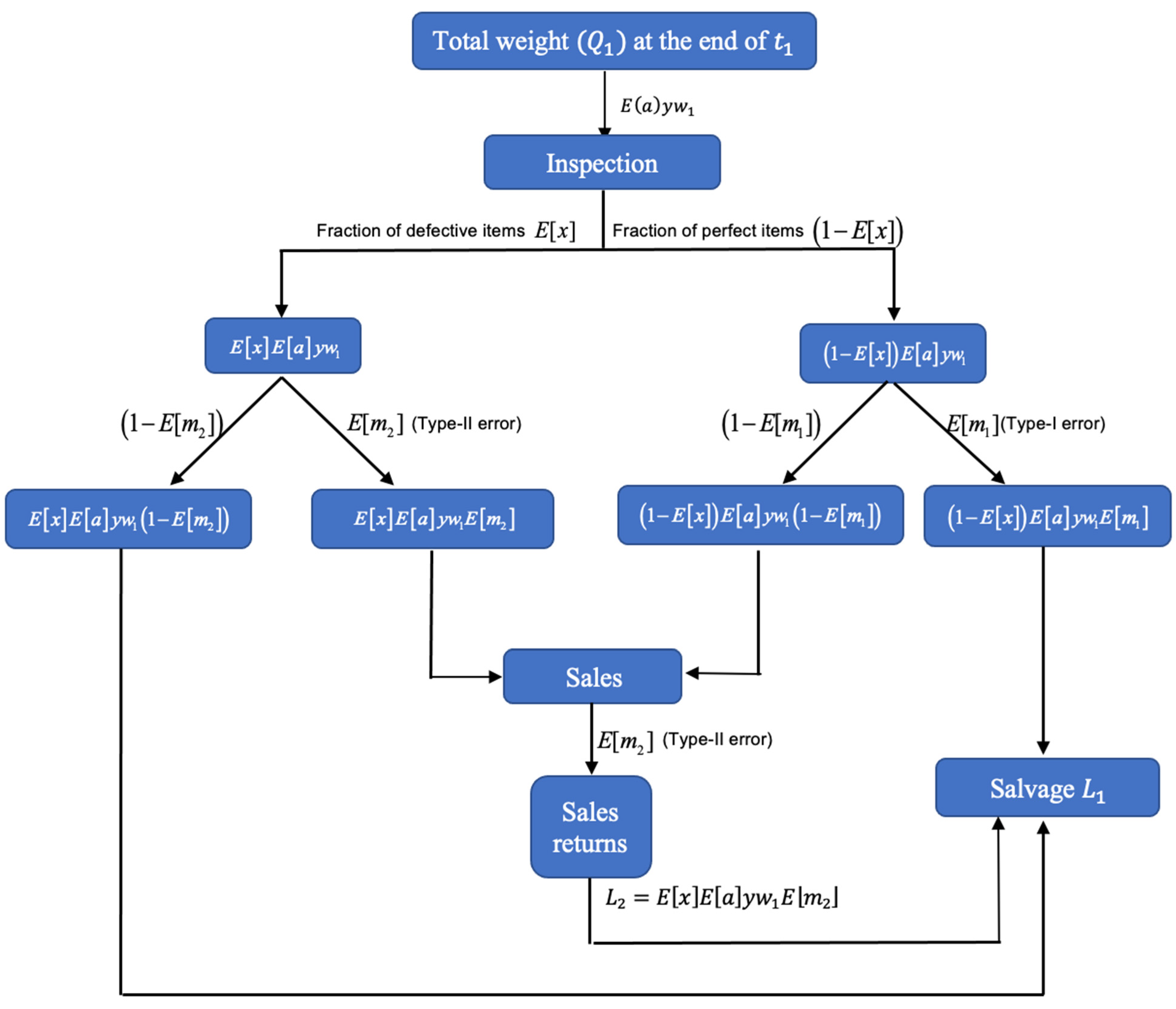
The inspection process is not assumed to be 100% effective because it results in Type-I errors (i.e., misclassifying a good item as defective) and Type-II errors (i.e., misclassifying a defective item as good);

(9)

Due to Type-II errors, a number of defective items are sold to customers as good items. So, when these items are returned and stored with items classified as defective by an inspector, they are salvaged at a cheaper price at the end of the inspection process;

(10)

The probability density functions, $g(x)$, $g(a)$, $g(m_1)$, and $g(m_2)$ are assumed to be known;

(11)

All returned items from customers are combined with those classified as defective by the inspector and are subsequently sold at a reduced price as a single batch at the end of each cycle;

(12)

The growing items exhibit a logistic growth function;

(13)

The shortages are allowed and are fully backordered;

(14)

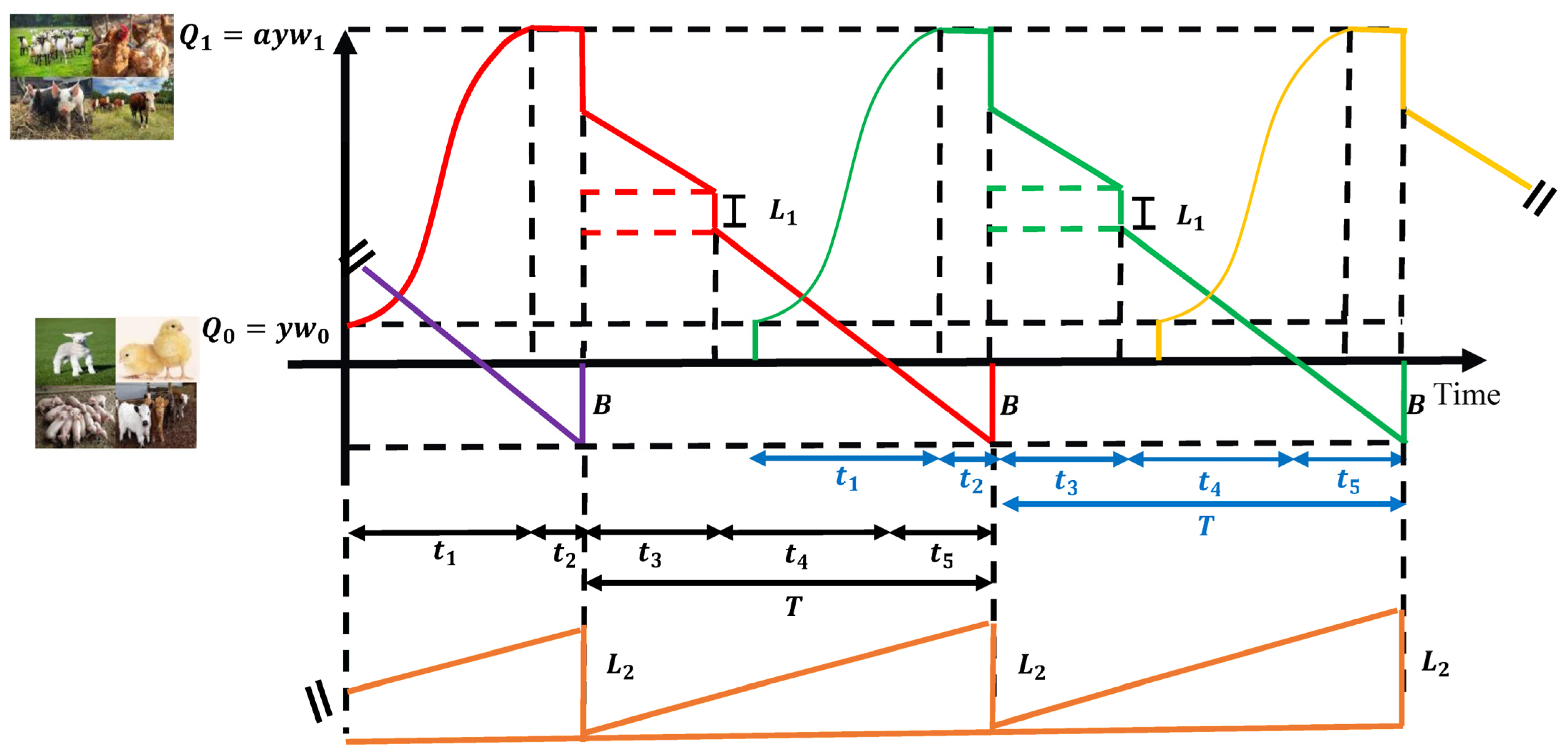
The items are slaughtered and immediately inspected to sell them to consumers. Initially, the backordering quantity is inspected to address the shortages from the previous cycle;

(15)

During the inspection period for the backordering quantity $t_2$, only $B$ units are initially inspected, and as soon as these $B$ units are ready, they are immediately delivered to the customer;

(16)

The holding cost for storing a weight unit of slaughtered items is incurred during both the backordering quantity inspection process and the consumption period;

(17)

The demand rate $D(s)$ follows a polynomial function that is dependent on the selling price of perfect-quality items. The function is expressed as $D(s)=\pi -\rho s^n$;

(18)

The selling price of perfect-quality items is optimized and must exceed the selling price of imperfect-quality items;

(19)

The inventory system takes into account carbon emissions, which are present in all operational processes except during the shortage period.

4. Mathematical Model

Figure 3 shows the behavior of the inventory system. The order quantity received $Q_0=y{w}_0$ grows in period $t_1$, then it is slaughtered at the end of this period when the items reach the target weight $Q_{t_1}=E\left[a\right]y{w}_1$. The fraction of live items that survive throughout the growth period $t_1$ is denoted by $a$. A fixed misclassification rate is used next. Specifically, a fraction $m_1$ of good items is incorrectly classified as defective, while a fraction $m_2$ of defective items is mistakenly classified as good. The inspection period for the backordering quantity $t_2$ is initiated to screen just the backordering quantity $B$ at rate $r$ to address the first shortages from the last cycle. For that reason, the inventory model decreases vertically by weight units $B$. The items continue to be screened at the same rate $r$ in the subsequent period $t_3$ until the total weight is inspected. The overall duration of the inspection process is denoted as $t_2+t_3$. It should be noted that during the period $t_3$, the on-hand inventory decreases due to the removal of imperfect items and the current demand rate. Additionally, it is assumed that the items returned from the market are stored together with those classified as defective by an inspector. Hence, at the end of period $t_3$, the imperfect items and the fraction of good items classified as defective are sold together as a single batch at a discounted price. As a result, $L_1=E\left[a\right]y{w}_1\left(1-E\left[x\right]\right)E\left[m_1\right]+E\left[x\right]E\left[a\right]y{w}_1\left(1-E\left[m_2\right]\right)$ is the batch classified as defective by an inspector, while $L_2=E\left[x\right]E\left[a\right]y{w}_{1}E\left[m_2\right]$ is the batch of units returned from the market accumulated over $T$ units of weight. Conversely, during period $t_4$, the inventory decreases solely due to the current demand rate. The inventory level continues to be consumed until it reaches zero at the end of period $t_4$, marking the start of the period of shortages. Finally, during period $t_5$, the shortages accumulate at the current demand rate and are eventually fulfilled in the subsequent cycle. The cycle time is obtained with $T=t_3+t_4+t_5$.

Throughout $t_1$, the items undergo a process of growth over time characterized by a logistic growth function that describes the relationship between the weight of the items and time. The logistic growth function depends on the asymptotic weight of the items $\alpha$, the integration constant $\beta$, and the growth rate $\lambda$, and is expressed as follows:

$$w_t\left(t\right)=\frac{\alpha }{1+\beta e^{-\lambda t}}$$

(1)

The growing items reach their desired weight of $w_1$ at the conclusion of the growth period $t_1$. Consequently, the items are slaughtered once they achieve this target weight. Thus,

$$w_1=w_t\left(t=t_1\right)=\frac{\alpha }{1+\beta e^{-\lambda t_1}}$$

(2)

The elapsed growing period ($t_1$) is given as

$$t_1=-\frac{\ln \left[\frac{1}{\beta }\left(\frac{\alpha }{w_1}-1\right)\right]}{\lambda }$$

(3)

Prior to being sold, the inventory requires inspection. Thus, the backordering quantity $B$ from the previous cycle must first undergo screening at an inspection rate $r$. The duration of the inspection period $t_2$ is determined by the following equation:

$$t_2=\frac{B}{r}$$

(4)

Following the inspection of the backordering quantity, the inspection period extends to cover the entire weight of the inventory. This inspection period occurs over the duration of the inspection time $t_3$, which is calculated as:

$$t_3=\frac{E\left[a\right]y{w}_1-B}{r}$$

(5)

After the screening process $t_3$, the identified defective items are removed from storage and sold at a lower cost. At this point, the remaining inventory consists solely of good items, which are consumed during $E\left[t_4\right]$. The time $E\left[t_4\right]$ is calculated as:

$$E\left[t_4\right]=\frac{E\left[a\right]y{w}_1\left[1-\left(1-E\left[x\right]\right)E\left[m_1\right]-E\left[x\right]\left(1-E\left[m_2\right]\right)\right]-B-D(s)t_3}{D(s)}$$

(6)

The shortage accumulation period ($t_5$) is calculated as:

$$t_5=\frac{B}{D(s)}$$

(7)

The expected cycle time $E\left[T\right]$ is computed by the sum of $t_3,t_4$, and $t_5$. Hence,

$$E\left[T\right]=t_3+E\left[t_4\right]+t_5=\frac{E\left[a\right]y{w}_1\left[1-\left(1-E\left[x\right]\right)E\left[m_1\right]-E\left[x\right]\left(1-E\left[m_2\right]\right)\right]}{D\left(s\right)}$$

(8)

An optimal inventory strategy is established based on the calculation of total revenues and total costs. The specific procedures for calculating each component of the total revenue and total cost are provided in the following sections.

4.1. Expected Sales Revenue per Cycle

The anticipated overall sales revenue is made up of two components. Throughout the cycle, the sale of good items is conducted at a unit weight price of $s$. This revenue includes cases where a good item is identified as such correctly, as well as Type-II error cases where a defective item is mistakenly identified as a good item. The revenue from good items is computed as:

$$R_1=sE\left[a\right]y{w}_1\left(1-E\left[x\right]\right)\left(1-E\left[m_1\right]\right)+sE\left[a\right]y{w}_{1}E\left[x\right]E\left[m_2\right]$$

(9)

The revenue generated from salvaging items is determined by the sum of $L_1+L_2$. $L_1$ occurs when a good item is mistakenly classified as defective, as well as in cases where a defective item is correctly identified as defective. On the other hand, $L_2$ represents situations in which a defective item is wrongly classified as a good item. The latter situation is considered because items in batch $L_2$ are returned by customers and stored together with those classified as imperfect quality in batch $L_1$. Consequently, these items are sold as a single batch at a reduced price of $v$ per unit of weight. Hence, the current revenue from salvaging items can be calculated as

$$R_2=L_1+L_2=vE\left[a\right]y{w}_1\left(1-E\left[x\right]\right)E\left[m_1\right]+vE\left[x\right]E\left[a\right]y{w}_1\left(1-E\left[m_2\right]\right)+vE\left[x\right]E\left[a\right]y{w}_{1}E\left[m_2\right]$$

or

$$R_2=vE\left[a\right]y{w}_1\left(1-E\left[x\right]\right)m_1+vE\left[x\right]E\left[a\right]y{w}_1$$

(10)

Therefore, using Equations (9) and (10), the expected sales revenue per cycle is $E\left[TR\right]=R_1+R_2$,

$$E\left[TR\right]=sE\left[a\right]y{w}_1\left(1-E\left[x\right]\right)\left(1-E\left[m_1\right]\right)+sE\left[a\right]y{w}_{1}E\left[x\right]m_2+vE\left[a\right]y{w}_1\left(1-E\left[x\right]\right)E\left[m_1\right]+vE\left[x\right]E\left[a\right]y{w}_1$$

(11)

4.2. Total Cost per Cycle

The anticipated overall cost $E\left[TC\right]$ per cycle comprises various cost components, including purchasing, setup, screening, rejecting a good item, accepting a defective item, feeding, mortality, holding live items, holding slaughtered items, backordering, and carbon emissions. The anticipated overall cost per cycle is determined as

$$E\left[TC\right]=Pc+Sc+Zc+c_{r}c+c_{a}c+Fc+Mc+hc+E\left[Hc\right]+Bc+E\left[Ec\right]$$

(12)

The projected final profit per cycle $E\left[TP\right]$ can be expressed as the difference between the expected total revenue $E\left[TR\right]$ per cycle and the anticipated overall cost per cycle $E\left[TC\right]$, that is:

$$E\left[TP\right]=E\left[TR\right]-Pc-Sc-Zc-c_{r}c-c_{a}c-Fc-Mc-hc-E\left[Hc\right]-Bc-E\left[Ec\right]$$

(13)

Consider now the multiple different costs of the inventory system.

4.3. Purchasing Cost per Cycle

At the start of each cycle, $y$ newborn items are procured at the price of $p$ per unit of weight. Upon receiving the order, each item has a weight of $w_0$. Thus, considering now multiple items the present purchasing cost is given as

$$Pc=py{w}_0$$

(14)

4.4. Setup Cost per Cycle

For the establishment of growing/feeding facilities, each cycle incurs a setup cost of $K$. Hence,

$$Sc=K$$

(15)

4.5. Screening Cost per Cycle

The screening cost per cycle encompasses both the screening process itself and the costs associated with misclassifications. To ensure the delivery of only high-quality products to customers, the screening process starts at time $t_2$ and continues until time $t_3$ a rate of $r$ with an inspection cost of $z$ per unit of weight. $c_r$ is the variable cost of rejecting a good item and $c_a$ is the variable cost of accepting a defective item. Thus, the present screening cost is denoted by:

$$Zc=zE\left[a\right]y{w}_1+c_{r}E\left[a\right]y{w}_1\left(1-E\left[x\right]\right)E\left[m_1\right]+c_{a}E\left[a\right]y{w}_{1}E\left[x\right]E\left[m_2\right]$$

(16)

4.6. Feeding Cost per Cycle

The feeding cost is determined based on several factors, including the cost of food for the items $c$, the general growth function $w_t\left(t\right)$, the feeding period duration (which is equivalent to the growing period, i.e., $t_1$) and the quantity of items in the facilities, $y$, which are used to obtain the feeding cost as

$$Fc=cE\left[a\right]y{\displaystyle \underset{0}{\overset{t_1}{\int }}{w}_{t_1}(t) dt}=cE\left[a\right]y{\displaystyle \underset{0}{\overset{t_1}{\int }}\left(\frac{\alpha }{1+\beta e^{-\lambda t}}\right) dt}=cE\left[a\right]y\left(\alpha t_1+\frac{\alpha }{\lambda }\left[\ln \left(1+\beta e^{-\lambda t_1}\right)-\ln \left(1+\beta \right)\right]\right)$$

(17)

4.7. Mortality Cost per Cycle

There is an expense incurred when discarding items that fail to reach a desired weight before perishing. The mortality cost per cycle $Mc$ is determined as the product of the average inventory level (i.e., the area under the graph of period $t_1$), the fraction of items which do not survive $\left(1-a\right)$, and the mortality cost $M$ per unit of weight. Hence,

$$Mc=M{\displaystyle {\int }_0^{t_1}\left(1-E\left[a\right]\right)y{w}_{t_1}\left(t\right)dt}=M\left(1-E\left[a\right]\right)y{\displaystyle {\int }_0^{t_1}\left(\frac{\alpha }{1+\beta e^{-\lambda t}}\right)dt}=M\left(1-E\left[a\right]\right)y\left\{\alpha T_f+\frac{\alpha }{\lambda }\left[\ln \left(1+\beta e^{-\lambda T_f}\right)-\ln \left(1+\beta \right)\right]\right\}$$

(18)

A company incurs two holding costs per cycle, i.e., the holding cost of slaughtered items and holding costs of live items.

4.8. Holding Cost of the Live Items per Cycle

During the growth period $t_1$, a company incurs a holding cost for the live items, which amounts to $h$ per unit of weight. Storage space is based on the weight of the items, as determined by the growth function $w_t\left(t\right)$. The holding cost of the live items per period can be calculated as:

$$hc=hE\left[a\right]y{\displaystyle \underset{0}{\overset{t_1}{\int }}{w}_{t_1}(t) dt}=hE\left[a\right]y{\displaystyle \underset{0}{\overset{t_1}{\int }}\left(\frac{\alpha }{1+\beta e^{-\lambda t}}\right) dt}=hE\left[a\right]y\left(\alpha t_1+\frac{\alpha }{\lambda }\left[\ln \left(1+\beta e^{-\lambda t_1}\right)-\ln \left(1+\beta \right)\right]\right)$$

(19)

4.9. Expected Holding Cost of Slaughtered Items per Cycle

The expected cost for holding the slaughtered items is incurred for the cycle time duration $T$. This cost is calculated as the product of the holding cost ($H$) per unit time per unit weight and the sum of the good lot, defective lot, and returned lot. The entire inventory held is determined by adding the areas $A_1+A_2+A_3+A_4+A_5+A_7$ (see Figure A1 in Appendix A). Therefore, the expression for the expected holding cost of the slaughtered items can be written as

$$\begin{array}{l}E\left[Hc\right]=H\left[BE\left[a\right]y{w}_1\left[1-\left(1-E\left[x\right]\right)E\left[m_1\right]-E\left[x\right]\left(1-E\left[m_2\right]\right)\right]\left[\frac{1}{r}-\frac{1}{D\left(s\right)}\right]\right.\\ +E\left[a^2\right]y^2{w}_{{}_1}^2\left[\frac{\left(1-E\left[x\right]\right)E\left[m_1\right]+E\left[x\right]\left(1-E\left[m_2\right]\right)}{r}+\frac{1-2\left[\left(1-E\left[x\right]\right)E\left[m_1\right]\right]+E\left[{\left(1-x\right)}^2\right]E\left[m_1^2\right]}{2D\left(s\right)}-\frac{\left[1-\left(1-E\left[x\right]\right)E\left[m_1\right]\right]\left[E\left[x\right]\left(1-E\left[m_2\right]\right)\right]}{D\left(s\right)}+\frac{E\left[x^2\right]E\left[{\left(1-m_2\right)}^2\right]}{2D\left(s\right)}\right]\\ +\frac{B^2}{2D\left(s\right)}+\frac{E\left[x\right]E\left[a\right]y{w}_{1}E\left[m_2\right]}{2}\left[\frac{E\left[a\right]y{w}_1\left[1-\left(1-E\left[x\right]\right)E\left[m_1\right]-E\left[x\right]\left(1-E\left[m_2\right]\right)\right]}{D\left(s\right)}\right]\end{array}$$

(20)

A comprehensive explanation of the calculation for the expected holding cost ($E\left[Hc\right]$) is provided in Appendix A.

4.10. Shortage Cost per Cycle

For time interval $t_5$, shortages are amassed until they attain the desired backordering quantity of $B$ units of weight. The cost associated with backordering is ascertained when multiplying the shortage cost ($b$) per unit of weight per unit of time by the area $A_6$ (see Figure A1 in Appendix A). Hence, the backordering cost can be given by:

$$Bc=\frac{b{B}^2}{2D(s)}$$

(21)

4.11. Carbon Emissions Produced by the Inventory System

The carbon emissions costs of the inventory system are initiated by every activity and can be obtained by multiplying the carbon tax rate $\theta$ (which is a recognized mechanism required by one of many government regulations acting as penalties) by the emissions from purchasing action $\stackrel{⌢}{P}c$, setup activity $\stackrel{⌢}{S}c$, screening process $\stackrel{⌢}{Z}c$, feeding process $\stackrel{⌢}{F}c$, mortality action $\stackrel{⌢}{M}c$, holding of the live items $\stackrel{⌢}{h}c$ and holding of the slaughtered items $E\left[\stackrel{⌢}{H}c\right]$.

The carbon emissions produced by purchasing actions are calculated as:

$$\stackrel{⌢}{P}c=\stackrel{⌢}{p}y{w}_0$$

(22)

The carbon emissions produced by the setup activity are calculated as:

$$\stackrel{⌢}{S}c=\stackrel{⌢}{K}$$

(23)

The carbon emissions produced by the screening process are calculated as:

$$\stackrel{⌢}{Z}c=\stackrel{⌢}{z}E\left[a\right]y{w}_1+{\stackrel{⌢}{c}}_{r}E\left[a\right]y{w}_1\left(1-E\left[x\right]\right)E\left[m_1\right]+{\stackrel{⌢}{c}}_{a}E\left[a\right]y{w}_{1}E\left[x\right]E\left[m_2\right]$$

(24)

The carbon emissions produced by the feeding process are calculated as:

$$\stackrel{⌢}{F}c=\stackrel{⌢}{c}E\left[a\right]y\underset{0}{\overset{t_1}{\int }}{w}_{t_1}(t) dt=\stackrel{⌢}{c}E\left[a\right]y{\displaystyle \underset{0}{\overset{t_1}{\int }}\left(\frac{\alpha }{1+\beta e^{-\lambda t}}\right) dt}=\stackrel{⌢}{c}E\left[a\right]y\left(\alpha t_1+\frac{\alpha }{\lambda }\left[\ln \left(1+\beta e^{-\lambda t_1}\right)-\ln \left(1+\beta \right)\right]\right)$$

(25)

The carbon emissions produced by the mortality action are calculated as:

$$\stackrel{⌢}{M}c=\stackrel{⌢}{M}{\displaystyle {\int }_0^{t_1}\left(1-E\left[a\right]\right)y{w}_{t_1}\left(t\right)dt}=\stackrel{⌢}{M}\left(1-E\left[a\right]\right)y{\displaystyle {\int }_0^{t_1}\left(\frac{\alpha }{1+\beta e^{-\lambda t}}\right)dt}=\stackrel{⌢}{M}\left(1-E\left[a\right]\right)y\left\{\alpha T_f+\frac{\alpha }{\lambda }\left[\ln \left(1+\beta e^{-\lambda T_f}\right)-\ln \left(1+\beta \right)\right]\right\}$$

(26)

The carbon emissions produced by inventory operations related to the holding of the live items are calculated as:

$$\stackrel{⌢}{h}c=\stackrel{⌢}{h}E\left[a\right]y{\displaystyle \underset{0}{\overset{t_1}{\int }}{w}_{t_1}(t) dt}=\stackrel{⌢}{h}E\left[a\right]y{\displaystyle \underset{0}{\overset{t_1}{\int }}\left(\frac{\alpha }{1+\beta e^{-\lambda t}}\right) dt}=\stackrel{⌢}{h}E\left[a\right]y\left(\alpha t_1+\frac{\alpha }{\lambda }\left[\ln \left(1+\beta e^{-\lambda t_1}\right)-\ln \left(1+\beta \right)\right]\right)$$

(27)

The carbon emissions produced by inventory operations related to the holding of the slaughtered items are calculated as:

$$\begin{array}{l}E\left[\stackrel{⌢}{H}c\right]=\stackrel{⌢}{H}\left[BE\left[a\right]y{w}_1\left[1-\left(1-E\left[x\right]\right)E\left[m_1\right]-E\left[x\right]\left(1-E\left[m_2\right]\right)\right]\left[\frac{1}{r}-\frac{1}{D\left(s\right)}\right]\right.\\ +E\left[a^2\right]y^2{w}_{{}_1}^2\left[\frac{\left(1-E\left[x\right]\right)E\left[m_1\right]+E\left[x\right]\left(1-E\left[m_2\right]\right)}{r}+\frac{1-2\left[\left(1-E\left[x\right]\right)E\left[m_1\right]\right]+E\left[{\left(1-x\right)}^2\right]E\left[m_1^2\right]}{2D\left(s\right)}-\frac{\left[1-\left(1-E\left[x\right]\right)E\left[m_1\right]\right]\left[E\left[x\right]\left(1-E\left[m_2\right]\right)\right]}{D\left(s\right)}+\frac{E\left[x^2\right]E\left[{\left(1-m_2\right)}^2\right]}{2D\left(s\right)}\right]\\ \left.+\frac{B^2}{2D\left(s\right)}+\frac{E\left[x\right]E\left[a\right]y{w}_{1}E\left[m_2\right]}{2}\left[\frac{E\left[a\right]y{w}_1\left[1-\left(1-E\left[x\right]\right)E\left[m_1\right]-E\left[x\right]\left(1-E\left[m_2\right]\right)\right]}{D\left(s\right)}\right]\right]\end{array}$$

(28)

All carbon emissions produced per time frame cost a company money. This cost is represented by:

$$\begin{array}{ll}Ec& =\theta \left[\stackrel{⌢}{p}y{w}_0 +\stackrel{⌢}{K}+\stackrel{⌢}{z}E\left[a\right]y{w}_1+{\stackrel{⌢}{c}}_{r}E\left[a\right]y{w}_1\left(1-E\left[x\right]\right)E\left[m_1\right]+{\stackrel{⌢}{c}}_{a}E\left[a\right]y{w}_{1}E\left[x\right]E\left[m_2\right]+y\left(\stackrel{⌢}{c}E\left[a\right]+\stackrel{⌢}{M}\left(1-E\left[a\right]\right)+\stackrel{⌢}{h}E\left[a\right]\right)\left(\alpha t_1+\frac{\alpha }{\lambda }\left[\ln \left(1+\beta e^{-\lambda t_1}\right)-\ln \left(1+\beta \right)\right]\right)\right.\hfill \\ & +\stackrel{⌢}{H}\left[BE\left[a\right]y{w}_1\left[1-\left(1-E\left[x\right]\right)E\left[m_1\right]-E\left[x\right]\left(1-E\left[m_2\right]\right)\right]\left[\frac{1}{r}-\frac{1}{D\left(s\right)}\right]\right.\\ & +E\left[a^2\right]y^2{w}_{{}_1}^2\left[\frac{\left(1-E\left[x\right]\right)E\left[m_1\right]+E\left[x\right]\left(1-E\left[m_2\right]\right)}{r}+\frac{1-2\left[\left(1-E\left[x\right]\right)E\left[m_1\right]\right]+E\left[{\left(1-x\right)}^2\right]E\left[m_1^2\right]}{2D\left(s\right)}-\frac{\left[1-\left(1-E\left[x\right]\right)E\left[m_1\right]\right]\left[E\left[x\right]\left(1-E\left[m_2\right]\right)\right]}{D\left(s\right)}+\frac{E\left[x^2\right]E\left[{\left(1-m_2\right)}^2\right]}{2D\left(s\right)}\right]\\ & \left.\left.+\frac{B^2}{2D\left(s\right)}+\frac{E\left[x\right]E\left[a\right]y{w}_{1}E\left[m_2\right]}{2}\left[\frac{E\left[a\right]y{w}_1\left[1-\left(1-E\left[x\right]\right)E\left[m_1\right]-E\left[x\right]\left(1-E\left[m_2\right]\right)\right]}{D\left(s\right)}\right]\right]\right]\end{array}$$

(29)

4.12. Expected Total Profit per Unit of Time

The expected total profit per unit of time $E\left[TPU\right]$ is calculated as the difference between the expected sales revenue per cycle $E\left[TR\right]$ and the expected total cost per cycle $E\left[TC\right]$. Therefore, the expected total profit per unit of time $E\left[TPU\right]$ is found by substituting Equations (11) and (14) into Equation (21), and Equation (29) into Equation (13). Finally, dividing the new $E\left[TP\right]$ function by the expected cycle time $E\left[T\right]$ results in $E\left[TPU\right]=\frac{E\left[TP\right]}{E\left[T\right]}$.

$$\begin{array}{l}E\left[TPU\right]=\frac{D\left(s\right)}{\left[1-\left(1-E\left[x\right]\right)E\left[m_1\right]-E\left[x\right]\left(1-E\left[m_2\right]\right)\right]}\left[s\left(1-E\left[x\right]\right)\left(1-E\left[m_1\right]\right)\right.+sE\left[x\right]E\left[m_2\right]+v\left(1-E\left[x\right]\right)E\left[m_1\right]+vE\left[x\right]\\ -\frac{p{w}_0}{E\left[a\right]w_1}-\frac{K}{E\left[a\right]y{w}_1}-z-c_r\left(1-E\left[x\right]\right)E\left[m_1\right]-c_{a}E\left[x\right]E\left[m_2\right]\\ \left.-\frac{\left(cE\left[a\right]+M\left(1-E\left[a\right]\right)+hE\left[a\right]\right)}{E\left[a\right]w_1}\left[\alpha t_1+\frac{\alpha }{\lambda }\left[\ln \left(1+\beta e^{-\lambda t_1}\right)-\ln \left(1+\beta \right)\right]\right]\right]\\ -H\left[\frac{E\left[a^2\right]y{w}_1}{2rE\left[a\right]\left[1-\left(1-E\left[x\right]\right)E\left[m_1\right]-E\left[x\right]\left(1-E\left[m_2\right]\right)\right]}\left[\left[2D\left(s\right)\left[\left(1-E\left[x\right]\right)E\left[m_1\right]+E\left[x\right]\left(1-E\left[m_2\right]\right)\right]\right]\right.\right.+\left[r\left[1-2\left[\left(1-E\left[x\right]\right)E\left[m_1\right]\right]+E\left[{\left(1-x\right)}^2\right]E\left[m_1^2\right]\right]\right]\\ \left.-\left[2r\left[1-\left(1-E\left[x\right]\right)E\left[m_1\right]\right]\left[E\left[x\right]\left(1-E\left[m_2\right]\right)\right]\right]+\left[rE\left[x^2\right]E\left[{\left(1-m_2\right)}^2\right]\right]\right]\\ +\frac{BD\left(s\right)}{r}-B+\frac{B^2}{2E\left[a\right]y{w}_1\left[1-\left(1-E\left[x\right]\right)E\left[m_1\right]-E\left[x\right]\left(1-E\left[m_2\right]\right)\right]}+\frac{E\left[x\right]E\left[a\right]y{w}_{1}E\left[m_2\right]}{2}{\displaystyle ]}\\ -\frac{b{B}^2}{2E\left[a\right]y{w}_1\left[1-\left(1-E\left[x\right]\right)E\left[m_1\right]-E\left[x\right]\left(1-E\left[m_2\right]\right)\right]}\\ -\theta \left[\frac{D\left(s\right)}{\left[1-\left(1-E\left[x\right]\right)E\left[m_1\right]-E\left[x\right]\left(1-E\left[m_2\right]\right)\right]}\right.\left[\frac{\stackrel{⌢}{p}{w}_0}{E\left[a\right]w_1}\right.+\frac{\stackrel{⌢}{K}}{E\left[a\right]y{w}_1}+\stackrel{⌢}{z}+{\stackrel{⌢}{c}}_r\left(1-E\left[x\right]\right)E\left[m_1\right]+{\stackrel{⌢}{c}}_{a}E\left[x\right]E\left[m_2\right]\\ +\left.\frac{\left(\stackrel{⌢}{c}E\left[a\right]-\stackrel{⌢}{M}\left(1-E\left[a\right]\right)-\stackrel{⌢}{h}E\left[a\right]\right)}{E\left[a\right]w_1}\left[\alpha t_1+\frac{\alpha }{\lambda }\left[\ln \left(1+\beta e^{-\lambda t_1}\right)-\ln \left(1+\beta \right)\right]\right]\right]\\ +\stackrel{⌢}{H}\left[\frac{E\left[a^2\right]y{w}_1}{2rE\left[a\right]\left[1-\left(1-E\left[x\right]\right)E\left[m_1\right]-E\left[x\right]\left(1-E\left[m_2\right]\right)\right]}\left[\left[2D\left(s\right)\left[\left(1-E\left[x\right]\right)E\left[m_1\right]+E\left[x\right]\left(1-E\left[m_2\right]\right)\right]\right]\right.\right.+\left[r\left[1-2\left[\left(1-E\left[x\right]\right)E\left[m_1\right]\right]+E\left[{\left(1-x\right)}^2\right]E\left[m_1^2\right]\right]\right]\\ \left.-\left[2r\left[1-\left(1-E\left[x\right]\right)E\left[m_1\right]\right]\left[E\left[x\right]\left(1-E\left[m_2\right]\right)\right]\right]+\left[rE\left[x^2\right]E\left[{\left(1-m_2\right)}^2\right]\right]\right]\\ \left.\left.+\frac{BD\left(s\right)}{r}-B+\frac{B^2}{2E\left[a\right]y{w}_1\left[1-\left(1-E\left[x\right]\right)E\left[m_1\right]-E\left[x\right]\left(1-E\left[m_2\right]\right)\right]}+\frac{E\left[x\right]E\left[a\right]y{w}_{1}E\left[m_2\right]}{2}\right]\right]\end{array}$$

(30)

As the expected total profit per unit time considers a demand rate that depends on a sale price with a polynomial function $D(s)=\pi -\rho s^n$, the expected total profit per unit of time $E\left[TPU\left(y,B,s\right)\right]$ becomes:

$$\begin{array}{l}E\left[TPU\right]=\frac{\left(\pi -\rho s^n\right)}{\left[1-\left(1-E\left[x\right]\right)E\left[m_1\right]-E\left[x\right]\left(1-E\left[m_2\right]\right)\right]}\left[s\left(1-E\left[x\right]\right)\left(1-E\left[m_1\right]\right)\right.+sE\left[x\right]E\left[m_2\right]+v\left(1-E\left[x\right]\right)E\left[m_1\right]+vE\left[x\right]\\ -\frac{p{w}_0}{E\left[a\right]w_1}-\frac{K}{E\left[a\right]y{w}_1}-z-c_r\left(1-E\left[x\right]\right)E\left[m_1\right]-c_{a}E\left[x\right]E\left[m_2\right]\\ \left.-\frac{\left(cE\left[a\right]+M\left(1-E\left[a\right]\right)+hE\left[a\right]\right)}{E\left[a\right]w_1}\left[\alpha t_1+\frac{\alpha }{\lambda }\left[\ln \left(1+\beta e^{-\lambda t_1}\right)-\ln \left(1+\beta \right)\right]\right]\right]\\ -H\left[\frac{E\left[a^2\right]y{w}_1}{2rE\left[a\right]\left[1-\left(1-E\left[x\right]\right)E\left[m_1\right]-E\left[x\right]\left(1-E\left[m_2\right]\right)\right]}\left[\left[2\left(\pi -\rho s^n\right)\left[\left(1-E\left[x\right]\right)E\left[m_1\right]+E\left[x\right]\left(1-E\left[m_2\right]\right)\right]\right]\right.\right.+\left[r\left[1-2\left[\left(1-E\left[x\right]\right)E\left[m_1\right]\right]+E\left[{\left(1-x\right)}^2\right]E\left[m_1^2\right]\right]\right]\\ \left.-\left[2r\left[1-\left(1-E\left[x\right]\right)E\left[m_1\right]\right]\left[E\left[x\right]\left(1-E\left[m_2\right]\right)\right]\right]+\left[rE\left[x^2\right]E\left[{\left(1-m_2\right)}^2\right]\right]\right]\\ \left.+\frac{B\left(\pi -\rho s^n\right)}{r}-B+\frac{B^2}{2E\left[a\right]y{w}_1\left[1-\left(1-E\left[x\right]\right)E\left[m_1\right]-E\left[x\right]\left(1-E\left[m_2\right]\right)\right]}+\frac{E\left[x\right]E\left[a\right]y{w}_{1}E\left[m_2\right]}{2}\right]\\ -\frac{b{B}^2}{2E\left[a\right]y{w}_1\left[1-\left(1-E\left[x\right]\right)E\left[m_1\right]-E\left[x\right]\left(1-E\left[m_2\right]\right)\right]}\\ -\theta \left[\frac{\left(\pi -\rho s^n\right)}{\left[1-\left(1-E\left[x\right]\right)E\left[m_1\right]-E\left[x\right]\left(1-E\left[m_2\right]\right)\right]}\right.\left[\frac{\stackrel{⌢}{p}{w}_0}{E\left[a\right]w_1}\right.+\frac{\stackrel{⌢}{K}}{E\left[a\right]y{w}_1}+\stackrel{⌢}{z}+{\stackrel{⌢}{c}}_r\left(1-E\left[x\right]\right)E\left[m_1\right]+{\stackrel{⌢}{c}}_{a}E\left[x\right]E\left[m_2\right]\\ +\left.\frac{\left(\stackrel{⌢}{c}E\left[a\right]+\stackrel{⌢}{M}\left(1-E\left[a\right]\right)+\stackrel{⌢}{h}E\left[a\right]\right)}{E\left[a\right]w_1}\left[\alpha t_1+\frac{\alpha }{\lambda }\left[\ln \left(1+\beta e^{-\lambda t_1}\right)-\ln \left(1+\beta \right)\right]\right]\right]\\ +\stackrel{⌢}{H}\left[\frac{E\left[a^2\right]y{w}_1}{2rE\left[a\right]\left[1-\left(1-E\left[x\right]\right)E\left[m_1\right]-E\left[x\right]\left(1-E\left[m_2\right]\right)\right]}\left[\left[2\left(\pi -\rho s^n\right)\left[\left(1-E\left[x\right]\right)E\left[m_1\right]+E\left[x\right]\left(1-E\left[m_2\right]\right)\right]\right]\right.\right.+\left[r\left[1-2\left[\left(1-E\left[x\right]\right)E\left[m_1\right]\right]+E\left[{\left(1-x\right)}^2\right]E\left[m_1^2\right]\right]\right]\\ \left.-\left[2r\left[1-\left(1-E\left[x\right]\right)E\left[m_1\right]\right]\left[E\left[x\right]\left(1-E\left[m_2\right]\right)\right]\right]+\left[rE\left[x^2\right]E\left[{\left(1-m_2\right)}^2\right]\right]\right]\\ \left.\left.+\frac{B\left(\pi -\rho s^n\right)}{r}-B+\frac{B^2}{2E\left[a\right]y{w}_1\left[1-\left(1-E\left[x\right]\right)E\left[m_1\right]-E\left[x\right]\left(1-E\left[m_2\right]\right)\right]}+\frac{E\left[x\right]E\left[a\right]y{w}_{1}E\left[m_2\right]}{2}\right]\right]\end{array}$$

(31)

Our target is to obtain the maximum expected total profit per unit of time $E\left[TPU\left(y,B,s\right)\right]$ by jointly optimizing the order quantity of newborn items, the backordering quantity, and the selling price of perfect items. Therefore, the optimization problem is represented by:

$$\begin{array}{l}\underset{\left(y,B,s\right)\in \mathrm{\Omega }}{Max} E\left[TPU\left(y,B,s\right)\right]\\ \mathrm{where} \mathrm{\Omega }=\left\{\left(y,B,s\right):y>0,0\le B\le y{w}_1 \mathrm{and} p\le s\le {\left(\frac{\pi }{\rho }\right)}^{\frac{1}{n}}\right\}\end{array}$$

(32)

5. Solution Procedure

Starting with an unconstrained optimization problem will allow for useful theoretical results. Next, the best values, $y^{*}$, $B^{*}$, and $s^{*}$, can be calculated in order to determine the max function of $E\left[TPU\left(y,B,s\right)\right]$. The required conditions of first-order derivatives shall hold, which provides the optimal values for y, B, and p:

$$\frac{\partial E\left[TPU(y,B,s)\right]}{\partial y}=0;\frac{\partial E\left[TPU(y,B,s)\right]}{\partial B}=0; \frac{\partial E\left[TPU(y,B,s)\right]}{\partial s}=0$$

(33)

This maximization formulation is a nonlinear optimization problem. Subsequently, the following numerical method is performed to find the global optimality of the model. By taking the first derivative of $E\left[TPU\left(y,B,s\right)\right]$ with respect to $y$, $B$, and $s$, we have:

$$\begin{array}{l}\frac{\partial E\left[TPU(y,B,s)\right]}{\partial y}=\frac{K\left(\pi -\rho s^n\right)}{E\left[a\right]y^2{w}_1\left[1-\left(1-E\left[x\right]\right)E\left[m_1\right]-E\left[x\right]\left(1-E\left[m_2\right]\right)\right]}+\frac{H{B}^2}{2E\left[a\right]y^2{w}_1\left[1-\left(1-E\left[x\right]\right)E\left[m_1\right]-E\left[x\right]\left(1-E\left[m_2\right]\right)\right]}+\frac{b{B}^2}{2E\left[a\right]y^2{w}_1\left[1-\left(1-E\left[x\right]\right)E\left[m_1\right]-E\left[x\right]\left(1-E\left[m_2\right]\right)\right]}\\ +\frac{\theta \stackrel{⌢}{K}\left(\pi -\rho s^n\right)}{E\left[a\right]y^2{w}_1\left[1-\left(1-E\left[x\right]\right)E\left[m_1\right]-E\left[x\right]\left(1-E\left[m_2\right]\right)\right]}+\frac{\theta \stackrel{⌢}{H}{B}^2}{2E\left[a\right]y^2{w}_1\left[1-\left(1-E\left[x\right]\right)E\left[m_1\right]-E\left[x\right]\left(1-E\left[m_2\right]\right)\right]}\\ -\left(H+\theta \stackrel{⌢}{H}\right)\left[\frac{\left(\pi -\rho s^n\right)E\left[a^2\right]w_1\left[\left(1-E\left[x\right]\right)E\left[m_1\right]+E\left[x\right]\left(1-E\left[m_2\right]\right)\right]}{rE\left[a\right]\left[1-\left(1-E\left[x\right]\right)E\left[m_1\right]-E\left[x\right]\left(1-E\left[m_2\right]\right)\right]}\right.+\frac{E\left[a^2\right]w_1\left[1-2\left[\left(1-E\left[x\right]\right)E\left[m_1\right]\right]+E\left[{\left(1-x\right)}^2\right]E\left[m_1^2\right]\right]}{2E\left[a\right]\left[1-\left(1-E\left[x\right]\right)E\left[m_1\right]-E\left[x\right]\left(1-E\left[m_2\right]\right)\right]}\\ -\frac{E\left[a^2\right]w_1\left[1-\left(1-E\left[x\right]\right)E\left[m_1\right]\right]\left[E\left[x\right]\left(1-E\left[m_2\right]\right)\right]}{E\left[a\right]\left[1-\left(1-E\left[x\right]\right)E\left[m_1\right]-E\left[x\right]\left(1-E\left[m_2\right]\right)\right]}+\frac{E\left[a^2\right]w_{1}E\left[x^2\right]E\left[{\left(1-m_2\right)}^2\right]}{2E\left[a\right]\left[1-\left(1-E\left[x\right]\right)E\left[m_1\right]-E\left[x\right]\left(1-E\left[m_2\right]\right)\right]}\\ \left.+\frac{E\left[x\right]E\left[a\right]w_{1}E\left[m_2\right]}{2}\right]=0\end{array}$$

(34)

$$\begin{array}{l}\frac{\partial \left[TPU(y,B,s)\right]}{\partial B}=-H\left[\frac{\left(\pi -\rho s^n\right)}{r}-1\right.\left.+\frac{B}{E\left[a\right]y{w}_1\left[1-\left(1-E\left[x\right]\right)E\left[m_1\right]-E\left[x\right]\left(1-E\left[m_2\right]\right)\right]}\right]\\ \\ -\frac{bB}{E\left[a\right]y{w}_1\left[1-\left(1-E\left[x\right]\right)E\left[m_1\right]-E\left[x\right]\left(1-E\left[m_2\right]\right)\right]}\\ -\theta \left[\stackrel{⌢}{H}\left.\left[\left.\frac{\left(\pi -\rho s^n\right)}{r}-1+\frac{B}{E\left[a\right]y{w}_1\left[1-\left(1-E\left[x\right]\right)E\left[m_1\right]-E\left[x\right]\left(1-E\left[m_2\right]\right)\right]}\right]\right.\right]\right.=0\end{array}$$

(35)

$$\begin{array}{l}\frac{\left[\pi -\left(n+1\right)\rho s^n\right]}{\left[1-\left(1-E\left[x\right]\right)E\left[m_1\right]-E\left[x\right]\left(1-E\left[m_2\right]\right)\right]}\left[\left(1-E\left[x\right]\right)\left(1-m_1\right)+E\left[x\right]m_2\right]-\frac{\rho n{s}^{n-1}}{w_1\left[1-\left(1-E\left[x\right]\right)E\left[m_1\right]-E\left[x\right]\left(1-E\left[m_2\right]\right)\right]}\left[v\left(1-E\left[x\right]\right)E\left[m_1\right]w_1+vE\left[x\right]w_1-\frac{\left(p+\theta \stackrel{⌢}{p}\right)w_0}{E\left[a\right]}-\frac{\left(K+\theta \stackrel{⌢}{K}\right)}{E\left[a\right]y}\right.\\ -\left(z+\theta \stackrel{⌢}{z}\right)w_1-\left(c_r+\theta {\stackrel{⌢}{c}}_r\right)\left(1-E\left[x\right]\right)E\left[m_1\right]w_1-\left(c_a+\theta {\stackrel{⌢}{c}}_a\right)E\left[x\right]E\left[m_2\right]w_1-\frac{\left[\left(c+\theta \stackrel{⌢}{c}\right)E\left[a\right]+\left(M+\theta \stackrel{⌢}{M}\right)\left(1-E\left[a\right]\right)+\left(h+\theta \stackrel{⌢}{h}\right)E\left[a\right]\right]}{E\left[a\right]}\left[\alpha t_1+\frac{\alpha }{\lambda }\left[\ln \left(1+\beta e^{-\lambda t_1}\right)-\ln \left(1+\beta \right)\right]\right]\\ \left.-\frac{\left(H+\theta \stackrel{⌢}{H}\right)}{rE\left[a\right]}\left[E\left[a^2\right]y{w}_1^2\left[\left(1-E\left[x\right]\right)E\left[m_1\right]+E\left[x\right]\left(1-E\left[m_2\right]\right)\right]+B{w}_1\left[1-\left(1-E\left[x\right]\right)E\left[m_1\right]-E\left[x\right]\left(1-E\left[m_2\right]\right)\right]E\left[a\right]\right]\right]=0\end{array}$$

(36)

Now, we take the second derivatives of Equations (34)–(36). The second order derivative of $E\left[TPU(y,B,s)\right]$ with respect to $y$ is calculated as:

$$\frac{{\partial }^{2}E\left[TPU(y,B,s)\right]}{\partial y^2}=-\frac{B^2\left[H+B+\theta \stackrel{⌢}{H}\right]+2\left(\pi -\rho s^n\right)\left[K+\theta \stackrel{⌢}{K}\right]}{E\left[a\right]y^3{w}_1\left[1-\left(1-E\left[x\right]\right)E\left[m_1\right]-E\left[x\right]\left(1-E\left[m_2\right]\right)\right]}<0$$

(37)

The second order derivative of $E\left[TPU(y,B,s)\right]$ with respect to $B$ is calculated as:

$$\frac{{\partial }^{2}E\left[TPU(y,B,s)\right]}{\partial B^2}=-\frac{H+b+\theta \stackrel{⌢}{H}}{E\left[a\right]y{w}_1\left[1-\left(1-E\left[x\right]\right)E\left[m_1\right]-E\left[x\right]\left(1-E\left[m_2\right]\right)\right]}<0$$

(38)

The second order derivative of $E\left[TPU(y,B,s)\right]$, with respect to $s$, is calculated as:

$$\begin{array}{l}\frac{{\partial }^{2}E\left[TPU(y,B,s)\right]}{\partial s^2}=-\frac{(n+1)\rho n{s}^{n-1}}{\left[1-\left(1-E\left[x\right]\right)E\left[m_1\right]-E\left[x\right]\left(1-E\left[m_2\right]\right)\right]}\left[\left(1-E\left[x\right]\right)\left(1-m_1\right)+E\left[x\right]m_2\right]-\frac{\rho n(n-1)s^{n-2}}{w_1\left[1-\left(1-E\left[x\right]\right)E\left[m_1\right]-E\left[x\right]\left(1-E\left[m_2\right]\right)\right]}\left[v\left(1-E\left[x\right]\right)E\left[m_1\right]w_1+vE\left[x\right]w_1-\frac{\left(p+\theta \stackrel{⌢}{p}\right)w_0}{E\left[a\right]}-\frac{\left(K+\theta \stackrel{⌢}{K}\right)}{E\left[a\right]y}\right.\\ -\left(z+\theta \stackrel{⌢}{z}\right)w_1-\left(c_r+\theta {\stackrel{⌢}{c}}_r\right)\left(1-E\left[x\right]\right)E\left[m_1\right]w_1-\left(c_a+\theta {\stackrel{⌢}{c}}_a\right)E\left[x\right]E\left[m_2\right]w_1-\frac{\left[\left(c+\theta \stackrel{⌢}{c}\right)E\left[a\right]+\left(M+\theta \stackrel{⌢}{M}\right)\left(1-E\left[a\right]\right)+\left(h+\theta \stackrel{⌢}{h}\right)E\left[a\right]\right]}{E\left[a\right]}\left[\alpha t_1+\frac{\alpha }{\lambda }\left[\ln \left(1+\beta e^{-\lambda t_1}\right)-\ln \left(1+\beta \right)\right]\right]\\ \left.-\frac{\left(H+\theta \stackrel{⌢}{H}\right)}{rE\left[a\right]}\left[E\left[a^2\right]y{w}_1^2\left[\left(1-E\left[x\right]\right)E\left[m_1\right]+E\left[x\right]\left(1-E\left[m_2\right]\right)\right]+B{w}_1\left[1-\left(1-E\left[x\right]\right)E\left[m_1\right]-E\left[x\right]\left(1-E\left[m_2\right]\right)\right]E\left[a\right]\right]\right]<0\end{array}$$

(39)

Next, the final equations for the second order cross partial derivatives can be calculated. The second order cross partial derivative ($\frac{{\partial }^2}{\partial y\partial B}$) of $E\left[TPU(y,B,s)\right]$ is given by:

$$\frac{{\partial }^{2}E\left[TPU(y,B,s)\right]}{\partial y\partial B}=\frac{B\left[H+b+\theta \stackrel{⌢}{H}\right]}{E\left[a\right]y^2{w}_1\left[1-\left(1-E\left[x\right]\right)E\left[m_1\right]-E\left[x\right]\left(1-E\left[m_2\right]\right)\right]}$$

(40)

The second order cross partial derivative ($\frac{{\partial }^2}{\partial y\partial s}$) of $E\left[TPU(y,B,s)\right]$ is given by:

$$\frac{{\partial }^{2}E\left[TPU(y,B,s)\right]}{\partial y\partial s}=-\frac{\rho n{s}^{n-1}}{E\left[a\right]y^2{w}_1\left[1-\left(1-E\left[x\right]\right)E\left[m_1\right]-E\left[x\right]\left(1-E\left[m_2\right]\right)\right]}\left(K+\theta \stackrel{⌢}{K}\right)+\frac{E\left[a^2\right]w_1\left[\left(1-E\left[x\right]\right)E\left[m_1\right]+E\left[x\right]\left(1-E\left[m_2\right]\right)\right]\rho n{s}^{n-1}}{rE\left[a\right]\left[1-\left(1-E\left[x\right]\right)E\left[m_1\right]-E\left[x\right]\left(1-E\left[m_2\right]\right)\right]}\left(H+\theta \stackrel{⌢}{H}\right)$$

(41)

The second order cross partial derivative ($\frac{{\partial }^2}{\partial B\partial y}$) of $E\left[TPU(y,B,s)\right]$ is given by:

$$\frac{{\partial }^{2}E\left[TPU(y,B,s)\right]}{\partial B\partial y}=\frac{B\left[H+b+\theta \stackrel{⌢}{H}\right]}{E\left[a\right]y^2{w}_1\left[1-\left(1-E\left[x\right]\right)E\left[m_1\right]-E\left[x\right]\left(1-E\left[m_2\right]\right)\right]}$$

(42)

The second order cross partial derivative ($\frac{{\partial }^2}{\partial B\partial s}$) of $E\left[TPU(y,B,s)\right]$ is given by:

$$\frac{{\partial }^{2}E\left[TPU(y,B,s)\right]}{\partial B\partial s}=\frac{\rho n{s}^{n-1}\left(H+\theta \stackrel{⌢}{H}\right)}{r}$$

(43)

The second order cross partial derivative ($\frac{{\partial }^2}{\partial s\partial y}$) of $E\left[TPU(y,B,s)\right]$ is given by:

$$\frac{{\partial }^{2}E\left[TPU(y,B,s)\right]}{\partial s\partial y}=-\frac{\rho n{s}^{n-1}}{E\left[a\right]y^2{w}_1\left[1-\left(1-E\left[x\right]\right)E\left[m_1\right]-E\left[x\right]\left(1-E\left[m_2\right]\right)\right]}\left(K+\theta \stackrel{⌢}{K}\right)+\frac{E\left[a^2\right]w_1\left[\left(1-E\left[x\right]\right)E\left[m_1\right]+E\left[x\right]\left(1-E\left[m_2\right]\right)\right]\rho n{s}^{n-1}}{rE\left[a\right]\left[1-\left(1-E\left[x\right]\right)E\left[m_1\right]-E\left[x\right]\left(1-E\left[m_2\right]\right)\right]}\left(H+\theta \stackrel{⌢}{H}\right)$$

(44)

The second order cross partial derivative ($\frac{{\partial }^2}{\partial s\partial B}$) of $E\left[TPU(y,B,s)\right]$ is

$$\frac{{\partial }^{2}E\left[TPU(y,B,s)\right]}{\partial s\partial B}=\frac{\rho n{s}^{n-1}\left(H+\theta \stackrel{⌢}{H}\right)}{r}$$

(45)

where the hessian matrix $H$ can be applied to obtain the second order partial derivatives, as shown below:

$$H=\left[\begin{array}{ccc}\frac{{\partial }^{2}E\left[TPU(y,B,s)\right]}{\partial y^2}& \frac{{\partial }^{2}E\left[TPU(y,B,s)\right]}{\partial y\partial B}& \frac{{\partial }^{2}E\left[TPU(y,B,s)\right]}{\partial y\partial s}\\ \frac{{\partial }^{2}E\left[TPU(y,B,s)\right]}{\partial B\partial y}& \frac{{\partial }^{2}E\left[TPU(y,B,s)\right]}{\partial B^2}& \frac{{\partial }^{2}E\left[TPU(y,B,s)\right]}{\partial B\partial s}\\ \frac{{\partial }^{2}E\left[TPU(y,B,s)\right]}{\partial s\partial y}& \frac{{\partial }^{2}E\left[TPU(y,B,s)\right]}{\partial s\partial B}& \frac{{\partial }^{2}E\left[TPU(y,B,s)\right]}{\partial s^2}\end{array}\right]$$

To prove the global optimality of the expected total profit per unit of time, which is comprised of three decision variables, the next statements must be true: $Det\left(H_1\right)<0,Det\left(H_2\right)>0$, and $Det\left(H_3\right)<0$, where $H_1$, $H_2$, and $H_3$ are the following matrices:

$$H_1=\left[\frac{{\partial }^{2}E\left[TPU(y,B,s)\right]}{\partial y^2}\right]$$

$$H_2=\left[\begin{array}{l}\frac{{\partial }^{2}E\left[TPU(y,B,s)\right]}{\partial y^2}\frac{{\partial }^{2}E\left[TPU(y,B,s)\right]}{\partial y\partial B}\\ \frac{{\partial }^{2}E\left[TPU(y,B,s)\right]}{\partial B\partial y}\frac{{\partial }^{2}E\left[TPU(y,B,s)\right]}{\partial B^2}\end{array}\right]$$

$$H_3=\left[\begin{array}{ccc}\frac{{\partial }^{2}E\left[TPU(y,B,s)\right]}{\partial y^2}& \frac{{\partial }^{2}E\left[TPU(y,B,s)\right]}{\partial y\partial B}& \frac{{\partial }^{2}E\left[TPU(y,B,s)\right]}{\partial y\partial s}\\ \frac{{\partial }^{2}E\left[TPU(y,B,s)\right]}{\partial B\partial y}& \frac{{\partial }^{2}E\left[TPU(y,B,s)\right]}{\partial B^2}& \frac{{\partial }^{2}E\left[TPU(y,B,s)\right]}{\partial B\partial s}\\ \frac{{\partial }^{2}E\left[TPU(y,B,s)\right]}{\partial s\partial y}& \frac{{\partial }^{2}E\left[TPU(y,B,s)\right]}{\partial s\partial B}& \frac{{\partial }^{2}E\left[TPU(y,B,s)\right]}{\partial s^2}\end{array}\right]$$

Hence,

$$Det\left(H_1\right)=\frac{{\partial }^{2}E\left[TPU(y,B,s)\right]}{\partial y^2}=-\frac{ B^2\left[H+b+\theta \stackrel{⌢}{H}\right]+2\left(\pi -\rho s^n\right)\left[K+\theta \stackrel{⌢}{K}\right]}{y^3{w}_1\left(1-E\left[x\right]\right)}<0$$

$$Det\left(H_2\right)=\left(\frac{{\partial }^{2}E\left[TPU(y,B,s)\right]}{\partial y^2}\right)\left(\frac{{\partial }^{2}E\left[TPU(y,B,s)\right]}{\partial B^2}\right)-{\left(\frac{{\partial }^{2}E\left[TPU(y,B,s)\right]}{\partial y\partial B}\right)}^{{}^2}>0$$

$$\begin{array}{l}Det\left(H_2\right)=\left(-\frac{ B^2\left[H+b+\theta \stackrel{⌢}{H}\right]+2\left(\pi -\rho s^n\right)\left[K+\theta \stackrel{⌢}{K}\right]}{y^3{w}_1\left(1-E\left[x\right]\right)}\right)\left(-\frac{H+b+\theta \stackrel{⌢}{H}}{y{w}_1\left(1-E\left[x\right]\right)}\right)\\ -{\left(\frac{B\left[H+b+\theta \stackrel{⌢}{H}\right]}{y^2{w}_1\left(1-E\left[x\right]\right)}\right)}^{{}^2}>0\end{array}$$

$$Det\left(H_2\right)=\left(\frac{ 2\left(\pi -\rho s^n\right)\left[K+\theta \stackrel{⌢}{K}\right]}{y^4{w}_{{}_1}^2{\left(1-E\left[x\right]\right)}^2}\right)\left(H+b+\theta \stackrel{⌢}{H}\right)>0$$

$$\begin{array}{ll}Det\left(H_3\right)& =\left(\frac{{\partial }^{2}E\left[TPU(y,B,s)\right]}{\partial y^2}\right)\left(\frac{{\partial }^{2}E\left[TPU(y,B,s)\right]}{\partial B^2}\right)\left(\frac{{\partial }^{2}E\left[TPU(y,B,s)\right]}{\partial s^2}\right)\\ & +\left(\frac{{\partial }^{2}E\left[TPU(y,B,s)\right]}{\partial B\partial y}\right)\left(\frac{{\partial }^{2}E\left[TPU(y,B,s)\right]}{\partial s\partial B}\right)\left(\frac{{\partial }^{2}E\left[TPU(y,B,s)\right]}{\partial y\partial s}\right)\\ & +\left(\frac{{\partial }^{2}E\left[TPU(y,B,s)\right]}{\partial s\partial y}\right)\left(\frac{{\partial }^{2}E\left[TPU(y,B,s)\right]}{\partial y\partial B}\right)\left(\frac{{\partial }^{2}E\left[TPU(y,B,s)\right]}{\partial B\partial s}\right)\\ & -\left(\frac{{\partial }^{2}E\left[TPU(y,B,s)\right]}{\partial y\partial s}\right)\left(\frac{{\partial }^{2}E\left[TPU(y,B,s)\right]}{\partial B^2}\right)\left(\frac{{\partial }^{2}E\left[TPU(y,B,s)\right]}{\partial s\partial y}\right)\\ & -\left(\frac{{\partial }^{2}E\left[TPU(y,B,s)\right]}{\partial B\partial s}\right)\left(\frac{{\partial }^{2}E\left[TPU(y,B,s)\right]}{\partial s\partial B}\right)\left(\frac{{\partial }^{2}E\left[TPU(y,B,s)\right]}{\partial y^2}\right)\\ & -\left(\frac{{\partial }^{2}E\left[TPU(y,B,s)\right]}{\partial s^2}\right)\left(\frac{{\partial }^{2}E\left[TPU(y,B,s)\right]}{\partial y\partial B}\right)\left(\frac{{\partial }^{2}E\left[TPU(y,B,s)\right]}{\partial B\partial y}\right) \mathrm{<} 0\end{array}$$

The previous calculation shows $E\left[TPU(y,B,s)\right]$ is strictly concave and proves that the Hessian is negative-definite. Consequently, a solution for the decision variables $\left(y^{*},B^{*},s^{*}\right)$ exists, is optimal, and maximizes the expected total profit. After some basic manipulations of the decision variables $y$ and $B$, we have:

$$y=\sqrt{\frac{2\left(\pi -\rho s^n\right)r\left[K+\theta \stackrel{⌢}{K}\right]}{\begin{array}{l}\left[w_1^2\left(H+\theta \stackrel{⌢}{H}\right)\right.\left[\left[2\left(\pi -\rho s^n\right)E\left[a^2\right]\left[\left(1-E\left[x\right]\right)E\left[m_1\right]+E\left[x\right]\left(1-E\left[m_2\right]\right)\right]\right]\right.+\left[rE\left[a^2\right]\left[1-2\left[\left(1-E\left[x\right]\right)E\left[m_1\right]\right]+E\left[{\left(1-x\right)}^2\right]E\left[m_1^2\right]\right]\right]\\ -\left[2rE\left[a^2\right]\left[1-\left(1-E\left[x\right]\right)E\left[m_1\right]\right]\left[E\left[x\right]\left(1-E\left[m_2\right]\right)\right]\right]+\left.\left[rE\left[a^2\right]E\left[x^2\right]E\left[{\left(1-m_2\right)}^2\right]\right]+\left.\left[rE\left[a\right]\left[1-\left(1-E\left[x\right]\right)E\left[m_1\right]-E\left[x\right]\left(1-E\left[m_2\right]\right)\right]E\left[x\right]E\left[a\right]E\left[m_2\right]\right]\right]\right]\\ -\frac{{\left[\left(H+\theta \stackrel{⌢}{H}\right)E\left[a\right]w_1\left[1-\left(1-E\left[x\right]\right)E\left[m_1\right]-E\left[x\right]\left(1-E\left[m_2\right]\right)\right]\left[r-\left(\pi -\rho s^n\right)\right]\right]}^2}{\left(H+b+\theta \stackrel{⌢}{H}\right)r}\end{array}}}$$

(46)

$$B=\frac{\left(H+\theta \stackrel{⌢}{H}\right)E\left[a\right]y{w}_1\left[1-\left(1-E\left[x\right]\right)E\left[m_1\right]-E\left[x\right]\left(1-E\left[m_2\right]\right)\right]\left[r-\left(\pi -\rho s^n\right)\right]}{\left(H+b+\theta \stackrel{⌢}{H}\right)r}$$

(47)

Solution Algorithm

The following Algorithm 1 finds the optimal values for the expected total profit per unit of time $E\left[TPU\right]$ and the three decision variables $\left(y^{*},B^{*},s^{*}\right)$ of the proposed inventory model:

Algorithm 1. Algoritm to obtain the optimal solution
Step 1.	Determine the input parameters of the inventory system.
Step 2.	Calculate selling price ($s^{\prime }$), order quantity ($y^{\prime }$), and backordering quantity ($B^{\prime }$) using Equations (36), (46) and (47), respectively.
Step 3.	If the optimality conditions are satisfied, continue to Step 4. Otherwise, skip to Step 8.
Step 4.	If $p\le s\le {\left(\frac{\pi }{\rho }\right)}^{\frac{1}{n}}$ is satisfied, apply Step 7. Otherwise, apply step 5.
Step 5.	If $s>{\left(\frac{\pi }{\rho }\right)}^{\frac{1}{n}}$, set $s^{\prime }={\left(\frac{\pi }{\rho }\right)}^{\frac{1}{n}}$, calculate order quantity ($y^{\prime }$) using Equation (46), calculate backordering quantity ($B^{\prime }$) using Equation (47), and go to Step 6. Otherwise, set $s^{\prime }=p$, calculate the order quantity ($y^{\prime }$) using Equation (46), calculate the backordering quantity ($B^{\prime }$) using Equation (47), and proceed to Step 6.
Step 6.	Use Equation (31) to determine the expected total profit per unit of time as $E\left[TPU\left(y^{\prime },B^{\prime },s^{\prime }\right)\right]$.
Step 7.	Solve for: $\left(y^{*},B^{*},s^{*}\right)=\left(y^{\prime },B^{\prime },s^{\prime }\right)$ and $E\left[TPU*\left(y^{*},B^{*},s^{*}\right)\right]=E\left[TPU\left(y^{\prime },B^{\prime },s^{\prime }\right)\right]$ and report the results.
Step 8.	End.

6. Numerical Example

To prove the solution approach and the applicability of the new proposed model, an example has been devised for broiler chicken, which is a specific type of newborn animal. To calculate the optimal order quantity of newborn items $\left(y^{*}\right)$, optimal backordering quantity $\left(B^{*}\right)$, optimal selling price of perfect items $\left(s^{*}\right)$, and expected value of total profit per unit of time $E\left[TPU*(y^{*},B^{*},s^{*})\right]$, a hypothetical data set has been defined that uses parameter values similar to those used in the inventory model proposed by Sebatjane and Adetunji [8]: $v=0.02$ $/g; $K=1000$ $/cycle; $c=0.2$ $/g/year; $p=0.025$ $/g; $z=0.00025$ $/g; $r=\mathrm{5,256,000}$ g/year; $\alpha =6870$ g; $\beta =120$; $\lambda =40$/year; $w_0=57$ g; $w_1=1500$ g; $x~U\left[\gamma ,\delta \right]$. From Alfares and Afzal [26], the holding cost of the live items is $h=0.4$ $/g/year and the holding cost of the slaughtered items is $H=0.8$ $/g/year. From Sebatjane and Adentuji [17], a mortality cost of $M=2$ $/g/year and $a~U\left[\tau ,\omega \right]$ are considered. The parameters $c_r$ and $c_a$ are taken from Khan et al. [54] but with different values, i.e., $c_r=0.05$ $/g, $c_a=0.25$ $/g, and with $m_1~U\left[\sigma ,\psi \right]$ and $m_2~U\left[\kappa ,\upsilon \right]$. We assume that the demand rate of growing items is given by a polynomial function $D(s)=\pi -\rho s^n$ and propose the following parameters with values of $\pi =\mathrm{135,000}$, $\rho =1050$, and $n=2$. The backordering cost is $b=$ 0.1 $/g/year. The relevant input parameters related to carbon emissions are $\theta =$0.0045 $/tons, $\stackrel{⌢}{K}=$ 2000 tons/year, $\stackrel{⌢}{H}=$ 0.8 tons/year, $\stackrel{⌢}{h}=$ 0.4 tons/year, $\stackrel{⌢}{c}=$ 0.65 tons/year, $\stackrel{⌢}{M}=$ 1 tons/year, $\stackrel{⌢}{p}=$ 0.375 tons/year, and $\stackrel{⌢}{z}=$ 0.005 tons/year, ${\stackrel{⌢}{c}}_r=$ 0.05 tons/year, ${\stackrel{⌢}{c}}_a=$ 0.25 tons/year. By applying the proposed algorithm, the resulting solution is optimal: $E\left[TPU*(y^{*},B^{*},s^{*})\right]=582256.9$ $/year; $y^{*}=30.29370$ units of newborn growing items; $B^{*}=\mathrm{34,176}.59$ g; and $s\ast =6.\mathrm{565,519}$ ZAR/g. The units of $y^{*}$ differ from the units $B^{*}$ becasue $y^{*}$ represents the number of items, whereas $B^{*}$ represents the quantity in weight (grams). The total weight is calculated as $Q_1=\left(y\right)\left(w_1\right)=$ 45,440.55 g. Therefore, $B<Q_1=$ 34,176.59 g < 45,440.55 g.

The fraction of imperfect items $x$, the fraction $a$ of live items that survived the growth period, the fraction of good items misclassified as defective $m_1$, and the fraction of defective items misclassified as good $m_2$, are random variables distributed uniformly over $\left[\gamma ,\delta \right]$, $\left[\tau ,\omega \right]$, $\left[\sigma ,\psi \right]$, and $\left[\kappa ,\upsilon \right]$, respectively. Their probability density functions are defined as:

Fraction of imperfect items $x$, with probability density function $f(x)$:

$$x~f(x)=\left\{\begin{array}{ll}\frac{1}{\delta -\gamma }& \gamma \le x\le \delta \\ 0& \mathrm{otherwise}\end{array}\right.$$

Considering $x~U\left[0,0.04\right]$

$$x~f(x)=\left\{\begin{array}{ll}25\hfill & 0\le x\le 0.04\hfill \\ 0\hfill & \mathrm{otherwise}\hfill \end{array}\right.$$

Then, $E\left[x\right]$, $E\left[x^2\right]$, $\left(1-E\left[x\right]\right)$ and $E\left[{\left(1-x\right)}^2\right]$ are computed as follows:

$$E\left[x\right]={\displaystyle \underset{\gamma }{\overset{\delta }{\int }}x f(x)dx=\frac{\gamma +\delta }{2}}=\frac{0+0.04}{2}=0.02$$

$$E\left[x^2\right]={\displaystyle \underset{\gamma }{\overset{\delta }{\int }}{x}^2 f(x)dx=\frac{{\gamma }^2+\gamma \delta +{\delta }^2}{3}}=\frac{0+(0)0.04+{0.04}^2}{3}=0.00053$$

$$E\left(1-x\right)={\displaystyle \underset{\gamma }{\overset{\delta }{\int }}\left(1-x\right) f(x)dx=\frac{2\delta -{\delta }^2-2\gamma +{\gamma }^2}{2\left(\delta -\gamma \right)}=}\frac{2\left(0.04\right)-{\left(0.04\right)}^2-2\left(0\right)+{\left(0\right)}^2}{2\left(0.04-0\right)}=0.98$$

$$E\left[{\left(1-x\right)}^2\right]={\displaystyle \underset{\gamma }{\overset{\delta }{\int }}{\left(1-x\right)}^2 f(x)dx=\frac{{\gamma }^2+\gamma \delta +{\delta }^2}{3}}+1-\gamma -\delta =\frac{0^2+0(0.04)+{(0.04)}^2}{3}+1-0-0.04=0.960533333$$

Fraction $a$ of live items that survived through the growth with probability density function $f(a)$:

$$a~f(a)=\left\{\begin{array}{ll}\frac{1}{\omega -\tau }& \tau \le a\le \omega \\ 0& \mathrm{otherwise}\end{array}\right.$$

Considering $a~U\left[0.8,1\right]$

$$a~f(a)=\left\{\begin{array}{ll}5\hfill & 0.8\le a\le 1\hfill \\ 1\hfill & \mathrm{otherwise}\hfill \end{array}\right.$$

Then, $E\left[a\right]$ and $E\left[a^2\right]$ are computed as follows:

$$E\left[a\right]={\displaystyle \underset{\tau }{\overset{\omega }{\int }}a f(a)da=\frac{\tau +\omega }{2}}=\frac{0.8+1}{2}=0.9$$

$$E\left[a^2\right]={\displaystyle \underset{\tau }{\overset{\omega }{\int }}{a}^2 f(a)da=\frac{{\tau }^2+\tau \omega +{\omega }^2}{3}}=\frac{{0.8}^2+(0.8)1+1^2}{3}=0.8133333$$

$$E\left(1-a\right)={\displaystyle \underset{\tau }{\overset{\omega }{\int }}\left(1-a\right) f(a)da=\frac{2\omega -{\omega }^2-2\tau +{\tau }^2}{2\left(\omega -\tau \right)}=}\frac{2\left(1\right)-{\left(1\right)}^2-2\left(0.8\right)+{\left(0.8\right)}^2}{2\left(1-0.8\right)}=0.1$$

The fraction of good items are classified as defective $m_1$, with probability density function $f(m_1)$:

$$m_1~f(m_1)=\left\{\begin{array}{ll}\frac{1}{\psi -\sigma }& \sigma \le m_1\le \psi \\ 0& \mathrm{otherwise}\end{array}\right.$$

Considering $m_1~U\left[0,0.05\right]$

$$m_1~f(m_1)=\left\{\begin{array}{ll}20 & 0\le m_1\le 0.05\\ 0& \mathrm{otherwise}\end{array}\right.$$

Then, $E\left[m_1\right]$, $E\left[m_1^2\right]$ and $\left(1-E\left[m_1\right]\right)$ are computed as follows:

$$E\left[m_1\right]={\displaystyle \underset{\sigma }{\overset{\psi }{\int }}{m}_1 f(m_1)d{m}_1=\frac{\sigma +\psi }{2}}=\frac{0+0.05}{2}=0.025$$

$$E\left[m_1^2\right]={\displaystyle \underset{\sigma }{\overset{\psi }{\int }}{m}_1^2 f(m_1)d{m}_1=\frac{{\sigma }^2+\sigma \psi +{\psi }^2}{3}}=\frac{0+(0)0.05+{0.05}^2}{3}=0.00083$$

$$E\left(1-m_1\right)={\displaystyle \underset{\sigma }{\overset{\psi }{\int }}\left(1-m_1\right) f(m_1)d{m}_1=\frac{2\psi -{\psi }^2-2\sigma +{\sigma }^2}{2\left(\psi -\sigma \right)}=\frac{2\left(0.05\right)-{\left(0.05\right)}^2-2\left(0\right)+{\left(0\right)}^2}{2\left(0.05-0\right)}}=0.975$$

Fraction of defective items classified as good $m_2$ with probability density function $f(m_2)$:

$$m_2~f(m_2)=\left\{\begin{array}{ll}\frac{1}{\upsilon -\kappa }& \kappa \le m_2\le \upsilon \\ 0& \mathrm{otherwise}\end{array}\right.$$

Considering $m_2~U\left[0,0.05\right]$

$$m_2~f(m_2)=\left\{\begin{array}{ll}20& 0\le m_2\le 0.05\\ 0& \mathrm{otherwise}\end{array}\right.$$

Then, $E\left[m_2\right]$, $\left(1-E\left[m_2\right]\right)$ and $E\left[{\left(1-m_2\right)}^2\right]$ are computed as follows:

$$E\left[m_2\right]={\displaystyle \underset{\kappa }{\overset{\upsilon }{\int }}{m}_2 f(m_2)d{m}_2=\frac{\kappa +\upsilon }{2}}=\frac{0+0.05}{2}=0.025$$

$$E\left(1-m_2\right)={\displaystyle \underset{\kappa }{\overset{\upsilon }{\int }}\left(1-m_2\right) f(m_2)d{m}_2=\frac{2\upsilon -{\upsilon }^2-2\kappa +{\kappa }^2}{2\left(\upsilon -\kappa \right)}}=\frac{2\left(0.05\right)-{\left(0.05\right)}^2-2\left(0\right)+{\left(0\right)}^2}{2\left(0.05-0\right)}=0.975$$

$$E\left[{\left(1-m_2\right)}^2\right]={\displaystyle \underset{\kappa }{\overset{\upsilon }{\int }}{\left(1-m_2\right)}^2 f(m_2)d{m}_2=\frac{{\kappa }^2+\kappa \upsilon +{\upsilon }^2}{3}}+1-\kappa -\upsilon =\frac{0^2+0(0.05)+{(0.05)}^2}{3}+1-0-0.05=0.9508333$$

Table 2. Comparison between the inventory model with and without a carbon emissions policy.

	Inventory Model
	With Carbon Emissions Policy	Without Carbon Emissions Policy
$TP$	582,256.9421	582,256.8876
$y$	30.29370	30.18259
$B$	34,176.59	34,034.27
$s$	6.565519	6.565373
Total Emissions	10,461.98	10,477.59

shows that the proposed model, which considers a carbon emissions policy, results in a higher total profit while the total number of emissions generated is lower than in a model that does not consider a carbon tax policy in its various activities. Therefore, the proposed model contributes positively to the environment and increases profits. When $\theta =0$, the target is to obtain a solution for the model that is optimal and does not consider an emissions policy. Then, the optimal solution is substituted in the utility function that considers an emissions policy to obtain the total profit and the total amount of carbon emissions for the model that does not consider a policy of carbon emissions. The total carbon emissions ($TCE$) are calculated as follows:

$$\begin{array}{l}TCE=\left[\frac{\left(\pi -\rho s^n\right)}{\left[1-\left(1-E\left[x\right]\right)E\left[m_1\right]-E\left[x\right]\left(1-E\left[m_2\right]\right)\right]}\right.\left[\frac{\stackrel{⌢}{p}{w}_0}{E\left[a\right]w_1}\right.+\frac{\stackrel{⌢}{K}}{E\left[a\right]y{w}_1}+\stackrel{⌢}{z}+{\stackrel{⌢}{c}}_r\left(1-E\left[x\right]\right)E\left[m_1\right]+{\stackrel{⌢}{c}}_{a}E\left[x\right]E\left[m_2\right]\\ +\left.\frac{\left(\stackrel{⌢}{c}E\left[a\right]+\stackrel{⌢}{M}\left(1-E\left[a\right]\right)+\stackrel{⌢}{h}E\left[a\right]\right)}{E\left[a\right]w_1}\left[\alpha t_1+\frac{\alpha }{\lambda }\left[\ln \left(1+\beta e^{-\lambda t_1}\right)-\ln \left(1+\beta \right)\right]\right]\right]\\ +\stackrel{⌢}{H}\left[\frac{E\left[a^2\right]y{w}_1}{2rE\left[a\right]\left[1-\left(1-E\left[x\right]\right)E\left[m_1\right]-E\left[x\right]\left(1-E\left[m_2\right]\right)\right]}\left[\left[2\left(\pi -\rho s^n\right)\left[\left(1-E\left[x\right]\right)E\left[m_1\right]+E\left[x\right]\left(1-E\left[m_2\right]\right)\right]\right]\right.\right.+\left[r\left[1-2\left[\left(1-E\left[x\right]\right)E\left[m_1\right]\right]+E\left[{\left(1-x\right)}^2\right]E\left[m_1^2\right]\right]\right]\\ \left.-\left[2r\left[1-\left(1-E\left[x\right]\right)E\left[m_1\right]\right]\left[E\left[x\right]\left(1-E\left[m_2\right]\right)\right]\right]+\left[rE\left[x^2\right]E\left[{\left(1-m_2\right)}^2\right]\right]\right]\\ \left.\left.+\frac{B\left(\pi -\rho s^n\right)}{r}-B+\frac{B^2}{2E\left[a\right]y{w}_1\left[1-\left(1-E\left[x\right]\right)E\left[m_1\right]-E\left[x\right]\left(1-E\left[m_2\right]\right)\right]}+\frac{E\left[x\right]E\left[a\right]y{w}_{1}E\left[m_2\right]}{2}\right]\right]\end{array}$$

Figure 4, Figure 5 and Figure 6 illustrate graphically that the expected total profit is a concave function. The figures also show that unique solutions exist for $y$, $B$, and $s$, which result in the maximization of the expected total profit. To prove the authenticity of the proposed model, a sensitivity analysis of the parameters is required.

7. Sensitivity Analysis

A sensitivity analysis of the model is conducted by varying the values of each of the main parameters between −40% and +40% (in increments of 20%). Table 2,

Table 3. Sensitivity analysis of the demand parameters, costs of the inventory system, and carbon emission parameters.

Parameters	% Change	y*		B*		s*		E[TPU*]
Base case		30.2937		34,176.59		6.56552		582,256.9
	−40	24.5287	−19.03	27,865.24	−18.47	5.0916	−22.45	269,021.3	−53.80
π	−20	0.0000	−100.00	0	−100.00	10.14185	54.47	2.05 × 108	35,135.98
	+20	32.5030	7.29	36,541.4	6.92	7.18989	9.51	766,566.9	31.65
	+40	34.4152	13.61	38,556.07	12.81	7.76415	18.26	967,061.9	66.09
	−40	30.3014	0.03	34,184.92	0.02	8.47051	29.02	753,705.8	29.45
ρ	−20	0.0000	−100.00	0	−100.00	12.67731	93.09	307.1733	−99.95
	+20	0.0000	−100.00	0	−100.00	10.35098	57.66	1,914,611	228.83
	+40	0.0000	−100.00	0	−100.00	9.58315	45.96	2.55 × 108	43,613.78
	−40	27.9737	−7.66	31,657.98	−7.37	29.69326	352.26	2,178,549	274.16
n	−20	0.0000	−100.00	0	−100.00	20.80728	216.92	3,328,837	471.71
	+20	0.0000	−100.00	0	−100.00	7.56502	15.22	7.18 × 107	12,236.69
	+40	31.4802	3.92	35,451.11	3.73	3.53205	−46.20	342,409.7	−41.19
	−40	30.2935	0.00	34,176.34	0.00	6.56564	0.00	582,223.5	−0.01
v	−20	30.2936	0.00	34,176.46	0.00	6.56558	0.00	582,240.2	0.00
	+20	30.2938	0.00	34,176.71	0.00	6.56546	0.00	582,273.6	0.00
	+40	30.2939	0.00	34,176.83	0.00	6.56539	0.00	582,290.3	0.01
	−40	23.5384	−22.30	26,555.24	−22.30	6.56318	−0.04	583,290.4	0.18
K	−20	27.1275	−10.45	30,604.47	−10.45	6.56442	−0.02	582,741.3	0.08
	+20	33.1584	9.46	37,408.59	9.46	6.56651	0.02	581,818.6	−0.08
	+40	35.7942	18.16	40,382.28	18.16	6.56742	0.03	581,415.4	−0.14
	−40	33.0344	9.05	34,725.54	1.61	6.56409	−0.02	582,640.9	0.07
H	−20	31.4843	3.93	34,568.64	1.15	6.56484	−0.01	582,431.9	0.03
	+20	29.3086	−3.25	33,684.19	−1.44	6.56614	0.01	582,101.4	−0.03
	+40	28.4582	−6.06	33,150.72	−3.00	6.56673	0.02	581,958.5	−0.05
	−40	30.2965	0.01	34,179.6	0.01	6.56399	−0.02	582,666.3	0.07
h	−20	30.2951	0.00	34,178.09	0.00	6.56476	−0.01	582,461.6	0.04
	+20	30.2923	0.00	34,175.08	0.00	6.56628	0.01	582,052.3	−0.04
	+40	30.2909	−0.01	34,173.57	−0.01	6.56704	0.02	581,847.6	−0.07
	−40	35.4564	17.04	41,853.72	22.46	6.56467	−0.01	582,931.2	0.12
b	−20	32.5149	7.33	37,512.75	9.76	6.56511	−0.01	582,573.3	0.05
	+20	28.5452	−5.77	31,506.64	−7.81	6.56591	0.01	581,973.3	−0.05
	+40	27.1261	−10.46	29,305.76	−14.25	6.56627	0.01	581,716.3	−0.09
	−40	30.2951	0.00	34,178.09	0.00	6.56476	−0.01	582,461.6	0.04
c	−20	30.2944	0.00	34,177.34	0.00	6.56514	−0.01	582,359.3	0.02
	+20	30.2930	0.00	34,175.83	0.00	6.5659	0.01	582,154.6	−0.02
	+40	30.2923	0.00	34,175.08	0.00	6.56628	0.01	582,052.3	−0.04
	−40	30.2953	0.01	34,178.26	0.00	6.56467	−0.01	582,484.4	0.04
M	−20	30.2945	0.00	34,177.42	0.00	6.5651	−0.01	582,370.6	0.02
	+20	30.2929	0.00	34,175.75	0.00	6.56594	0.01	582,143.2	−0.02
	+40	30.2922	−0.01	34,174.91	0.00	6.56637	0.01	582,029.5	−0.04
	−40	30.2940	0.00	34,176.88	0.00	6.56537	0.00	582,296.6	0.01
P	−20	30.2938	0.00	34,176.73	0.00	6.56545	0.00	582,276.7	0.00
	+20	30.2936	0.00	34,176.44	0.00	6.56559	0.00	582,237.1	0.00
	+40	30.2934	0.00	34,176.29	0.00	6.56567	0.00	582,217.3	−0.01
	−40	30.2938	0.00	34,176.66	0.00	6.56548	0.00	582,266.3	0.00
Z	−20	30.2937	0.00	34,176.62	0.00	6.5655	0.00	582,261.6	0.00
	+20	30.2937	0.00	34,176.55	0.00	6.56554	0.00	582,252.2	0.00
	+40	30.2936	0.00	34,176.52	0.00	6.56555	0.00	582,247.5	0.00
	−40	30.2940	0.00	34,176.92	0.00	6.56535	0.00	582,302.9	0.01
cr	−20	30.2939	0.00	34,176.76	0.00	6.56543	0.00	582,279.9	0.00
	+20	30.2935	0.00	34,176.42	0.00	6.5656	0.00	582,233.9	0.00
	+40	30.2934	0.00	34,176.25	0.00	6.56569	0.00	582,210.9	−0.01
	−40	30.2937	0.00	34,176.62	0.00	6.5655	0.00	582,261.6	0.00
ca	−20	30.2937	0.00	34,176.6	0.00	6.56551	0.00	582,259.3	0.00
	+20	30.2937	0.00	34,176.57	0.00	6.56553	0.00	582,254.6	0.00
	+40	30.2937	0.00	34,176.55	0.00	6.56554	0.00	582,252.2	0.00
θ	−40	30.2493	−0.15	34,119.76	−0.17	6.56546	0.00	582,275.8	0.00
	−20	30.2715	−0.07	34,148.19	−0.08	6.56549	0.00	582,266.3	0.00
	+20	30.3158	0.07	34,204.95	0.08	6.56555	0.00	582,247.5	0.00
	+40	30.3379	0.15	34,233.28	0.17	6.56558	0.00	582,238.1	0.00
	−40	30.2396	−0.18	34,115.6	−0.18	6.5655	0.00	582,265.2	0.00
$K$	−20	30.2667	−0.09	34,146.11	−0.09	6.56551	0.00	582,261.1	0.00
	+20	30.3207	0.09	34,207.04	0.09	6.56553	0.00	582,252.8	0.00
	+40	30.3477	0.18	34,237.46	0.18	6.56554	0.00	582,248.7	0.00
	−40	30.3034	0.03	34,180.69	0.01	6.56551	0.00	582,258.4	0.00
$\stackrel{⌢}{H}$	−20	30.2985	0.02	34,178.64	0.01	6.56552	0.00	582,257.7	0.00
	+20	30.2889	−0.02	34,174.53	−0.01	6.56552	0.00	582,256.2	0.00
	+40	30.2841	−0.03	34,172.48	−0.01	6.56552	0.00	582,255.5	0.00
	−40	30.2937	0.00	34,176.6	0.00	6.56551	0.00	582,258.8	0.00
$\stackrel{⌢}{h}$	−20	30.2937	0.00	34,176.59	0.00	6.56552	0.00	582,257.9	0.00
	+20	30.2937	0.00	34,176.58	0.00	6.56552	0.00	582,256	0.00
	+40	30.2937	0.00	34,176.57	0.00	6.56553	0.00	582,255.1	0.00
	−40	30.2937	0.00	34,176.61	0.00	6.56551	0.00	582,259.9	0.00
$\stackrel{⌢}{c}$	−20	30.2937	0.00	34,176.6	0.00	6.56551	0.00	582,258.4	0.00
	+20	30.2937	0.00	34,176.58	0.00	6.56552	0.00	582,255.4	0.00
	+40	30.2937	0.00	34,176.56	0.00	6.56553	0.00	582,253.9	0.00
	−40	30.2937	0.00	34,176.59	0.00	6.56552	0.00	582,257.4	0.00
$\stackrel{⌢}{M}$	−20	30.2937	0.00	34,176.59	0.00	6.56552	0.00	582,257.2	0.00
	+20	30.2937	0.00	34,176.58	0.00	6.56552	0.00	582,256.7	0.00
	+40	30.2937	0.00	34,176.58	0.00	6.56552	0.00	582,256.4	0.00
	−40	30.2937	0.00	34,176.61	0.00	6.56551	0.00	582,259.6	0.00
$\stackrel{⌢}{p}$	−20	30.2937	0.00	34,176.6	0.00	6.56551	0.00	582,258.3	0.00
	+20	30.2937	0.00	34,176.58	0.00	6.56552	0.00	582,255.6	0.00
	+40	30.2937	0.00	34,176.57	0.00	6.56553	0.00	582,254.3	0.00
	−40	30.2937	0.00	34,176.59	0.00	6.56552	0.00	582,257.8	0.00
$\stackrel{⌢}{z}$	−20	30.2937	0.00	34,176.59	0.00	6.56552	0.00	582,257.4	0.00
	+20	30.2937	0.00	34,176.58	0.00	6.56552	0.00	582,256.5	0.00
	+40	30.2937	0.00	34,176.58	0.00	6.56552	0.00	582,256.1	0.00
	−40	30.2937	0.00	34,176.59	0.00	6.56552	0.00	582,257.1	0.00
${\stackrel{⌢}{c}}_r$	−20	30.2937	0.00	34,176.59	0.00	6.56552	0.00	582,257	0.00
	+20	30.2937	0.00	34,176.59	0.00	6.56552	0.00	582,256.8	0.00
	+40	30.2937	0.00	34,176.58	0.00	6.56552	0.00	582,256.7	0.00
	−40	30.2937	0.00	34,176.59	0.00	6.56552	0.00	582,257	0.00
${\stackrel{⌢}{c}}_a$	−20	30.2937	0.00	34,176.59	0.00	6.56552	0.00	582,256.9	0.00
	+20	30.2937	0.00	34,176.59	0.00	6.56552	0.00	582,256.9	0.00
	+40	30.2937	0.00	34,176.59	0.00	6.56552	0.00	582,256.9	0.00
	−40	30.2841	−0.03	34,166.2	−0.03	6.57078	0.08	580,846.2	−0.24
λ	−20	30.2901	−0.01	34,172.69	−0.01	6.56749	0.03	581,727.8	−0.09
	+20	30.2961	0.01	34,179.18	0.01	6.56420	−0.02	582,609.8	0.06
	+40	30.2978	0.01	34,181.03	0.01	6.56327	−0.03	582,861.9	0.10
w1	−40	50.4905	66.67	34,177.23	0.00	6.56519	−0.01	582,345.1	0.02
	−20	37.8675	25.00	34,176.94	0.00	6.56534	0.00	582,305.6	0.01
	+20	25.2444	−16.67	34,176.18	0.00	6.56573	0.00	582,201.3	−0.01
	+40	21.6378	−28.57	34,175.72	0.00	6.56596	0.01	582,139.4	−0.02

,

Table 4. Effect of $x$ on $E\left[TPU(y,B,s)\right]$ when the defective probability $x$ is distributed uniformly between $\gamma$ and $\delta$.

Parameters	% Change	y*		B*		s*		E[TPU*]
Base case		30.2937		34,176.59		6.56552		582,256.9
	−40	30.0826	−0.7	34,208.19	0.09	6.56547	0.00	582,268.5	0.00
E[x]	−20	30.1861	−0.36	34,190.52	0.04	6.56549	0.00	582,262.5	0.00
	+20	30.4056	0.37	34,166.46	−0.03	6.56554	0.00	582,251.9	0.00
	+40	30.5218	0.75	34,160.21	−0.05	6.56557	0.00	582,247.3	0.00

and

Table 5. Effect of $m_1$ on $E\left[TPU(y,B,s)\right]$ when the defective probability $m_1$ is uniformly distributed between $\sigma$ and $\psi$.

Parameters	% Change	y*		B*		s*		E[TPU*]
Base case		30.2937		34,176.59		6.56552		582,256.9
	−40	29.9859	−1.02	34,176.15	0.00	6.56531	0.00	582,307.6	0.01
E[m1]	−20	30.1364	−0.52	34,173.33	−0.01	6.56541	0.00	582,282	0.00
	+20	30.4583	0.54	34,186.12	0.03	6.56563	0.00	582,232.5	0.00
	+40	30.6303	1.11	34,202.13	0.07	6.56573	0.00	582,208.6	−0.01

show the impact of using different input parameters on the values of the expected total profit per unit of time, order quantity, backordering quantity, and selling price of growing items. Moreover, the impact of the fluctuations on the optimal values of $TC\ast$, $y\ast$ and $t\ast$ with respect to the input parameters is depicted in Figure 7, Figure 8 and Figure 9.

Table 3 shows that of all the parameters tested, only the scale parameter $\pi$ of the price-dependent demand, the sensitivity parameter $\rho$, and the demand power index $n$ are very sensitive. Additionally, the maximum total profit lying within the profit drop is −53.80%, while profit growth is 43,613.78%. The setup cost parameter $K$ is moderately sensitive because it affects the profit within the range [−0.14%, 0.18%]. Table 3 also shows that the total profit is less sensitive to changes in the other parameters by maintaining the parameter values within the bounds of around ±20% exclusively.

The results in Table 4 show that, as the portion of items with imperfect quality (x) grows, the number of items that are classified as good decreases. To equalize this effect, the size of the order quantity of newborn items increases. Table 4 also shows that the company experiences a decrease in optimal backorder quantity and optimum profit, coupled with a small increase in the selling price of perfect items. In summary, the increase in defective items in the system forces a company to raise prices to counteract the loss of sales.

Table 5 shows that the increase in the Type-I error results in an increase in the order quantity of newborn items, the backordering quantity, and the selling price of perfect items. However, the expected total profit tends to fall with this kind of error. As a result, the company cannot sell all the perfect items and erroneously dismisses some of them as imperfect, which prevents the maximum possible sales from being achieved and reduces the expected total profits considerably. In addition, the loss accrued by the inspection error is compensated by a small increase in the selling price.

From

Table 6. Effect of $m_2$ on $E\left[TPU(y,B,s)\right]$ when the defective probability $m_2$ is uniformly distributed between $\kappa$ and $\upsilon$.

Parameters	% Change	y*		B*		s*		E[TPU*]
Base case		30.2937		34,176.59		6.56552		582,256.9
	−40	30.3216	0.09	34,200.92	0.07	6.56550	0.00	582,264.5	0.00
E[m2]	−20	30.3077	0.05	34,188.75	0.04	6.56551	0.00	582,260.7	0.00
	+20	30.2798	−0.05	34,164.44	−0.04	6.56553	0.00	582,253.2	0.00
	+40	30.2659	−0.09	34,152.32	−0.07	6.56554	0.00	582,249.4	0.00

, the negative correlation between the fraction of Type-II error ($m_2$) and both the order quantity of newborn items (y*) and the optimal backordering quantity (B*) can be observed. What this means in practical terms is that the size of the order quantity and the backorder quantity must be decreased as the number of items that are chosen as good increases. This effect is due to frustration and dissatisfaction with quality, as customers may not want to buy more. The increase in the selling price of perfect items is a valid tactic to increase sales in a deficient environment.

Figure 7 confirms that the order quantity of newborn items and the fraction of imperfect items are very sensitive to changes in the Type-I error. In other words, as the fraction of imperfect items increases, the order quantity of the newborn items also has to increase to fulfill the demand. Conversely, the order quantity of newborn items is less susceptible to changes in the Type-II error because anytime a defective item is classified as good, the size of the order is reduced.

Figure 8 shows that as the fraction of imperfect items decreases, so does the number of pending orders. Therefore, if the number of defective items is predicted correctly, a company is in a better position to reduce the number of pending orders. The same type of correlation is observed with the Type-II error because shortages are covered with bad items that were erroneously classified as good. Figure 8 also shows that the backordering quantity is highly sensitive to the Type-I error because items that were good are classified as bad and can potentially prevent the company from fulfilling customer orders on time.

Figure 9 reveals that when the changes in the Type-II error and the fraction of imperfect items range between −40 and +40%, the selling price of perfect items stays almost the same. The selling price of perfect items has a positive correlation with the Type-I error and ranges between USD 6.5653 and USD 6.56575.

Figure 10 shows that when the Type-I error increases, the expected total profit decreases. This is because classifying good items as defective induces a drop in revenue. In addition, the drop in revenue resulting from lower sales is not the only concern since the system incurs extra costs as these items accumulate. On the other hand, the Type-II error decreases the expected total profit.

8. Managerial Insights

To increase the performance of the inventory model for growing items, several key points derived from the results obtained by solving the model and sensitivity analyses are highlighted for management to implement:

• It is recommended that the cause of the imperfections be identified through defect tracking and root cause analysis to lower the fraction of defects, since one can expect higher total profits by addressing these process deficiencies;
• It is beneficial to reduce the fraction of good items classified as defective (i.e., Type-I error), since the sensitivity analysis suggests a direct impact on sales resulting from this type of error;
• When a fraction of defective items is classified as good (i.e., Type-II error), some undesirable effects can be seen, including a higher return rate, which, in turn, translates into extra costs for a company (e.g., penalties, loss of customer confidence, etc.). Therefore, the fraction of Type-II error (q2) must be lowered since the total expected profit is directly impacted by this type of error;
• The results showed that the cost of feeding is the main contributor to reducing the expected total profits. Farmers looking to decrease total costs need to understand the impact of feeding costs when compared to other possible influencing parameters.

9. Conclusions and Future Research Directions

In real-life situations, it is impossible to ensure that 100% of the manufactured items will be of perfect quality or that inspectors will not make mistakes. Therefore, it is necessary to identify and control Type-I and Type-II errors to the greatest extent. This paper explored and presented a new mathematical model for growing items with inspection errors, imperfect quality, carbon emissions, and planned backorders. The goal of the mathematical model is to optimize multiple parameters, such as the order quantity of newborn items, the selling price of perfect items, and the backordering quantity. A numerical example is used in conjunction with a full sensitivity analysis to demonstrate the pragmatism of this model. Future research could incorporate additional parameters into the model, including inflation, payment delays, and return of sales, to name a few. Multiple demand functions could also be explored to extend the study.

References

1. Harris, F.W. How many parts to make at once. Fact. Mag. Manag. 1913, 152, 135–136. [Google Scholar] [CrossRef]
2. Rezaei, J. Economic order quantity for growing items. Int. J. Prod. Econ. 2014, 155, 109–113. [Google Scholar] [CrossRef]
3. Ritha, W.; Haripriya, S. Inventory model on organic poultry farming. Int. J. Res. Eng. Appl. Sci. 2015, 5, 30–38. [Google Scholar]
4. Zhang, Y.; Li, L.-Y.; Tian, X.-Q.; Feng, C. Inventory management research for growing items with carbon-constrained. In Proceedings of the 2016 35th Chinese Control Conference (CCC), Chengdu, China, 27–29 July 2016; pp. 9588–9593. [Google Scholar] [CrossRef]
5. Dhanam, K.; Jesintha, W. Fuzzy inventory model for slow and fast growing items with deterioration constraints in a single period. Int. J. Manag. Soc. Sci. 2017, 5, 308–317. [Google Scholar]
6. Sebatjane, M. Selected Deterministic Models for Lot Sizing of Growing Items Inventory. Master’s Thesis, University of Pretoria, Pretoria, South Africa, 2018. [Google Scholar]
7. Nobil, A.H.; Sedigh, A.H.A.; Cárdenas-Barrón, L.E. A Generalized Economic Order Quantity Inventory Model with Shortage: Case Study of a Poultry Farmer. Arab. J. Sci. Eng. 2019, 44, 2653–2663. [Google Scholar] [CrossRef]
8. Sebatjane, M.; Adetunji, O. Economic order quantity model for growing items with imperfect quality. Oper. Res. Perspect. 2018, 6, 100088. [Google Scholar] [CrossRef]
9. Sebatjane, M.; Adetunji, O. Economic order quantity model for growing items with incremental quantity discounts. J. Ind. Eng. Int. 2019, 15, 545–556. [Google Scholar] [CrossRef]
10. Sebatjane, M.; Adetunji, O. Three-echelon supply chain inventory model for growing items. J. Model. Manag. 2019, 15, 567–587. [Google Scholar] [CrossRef]
11. Khalilpourazari, S.; Pasandideh, S.H.R. Modeling and optimization of multi-item multi-constrained EOQ model for growing items. Knowl.-Based Syst. 2019, 164, 150–162. [Google Scholar] [CrossRef]
12. Malekitabar, M.; Yaghoubi, S.; Gholamian, M.R. A novel mathematical inventory model for growing-mortal items (case study: Rainbow trout). Appl. Math. Model. 2019, 71, 96–117. [Google Scholar] [CrossRef]
13. Nobil, A.; Taleizadeh, A.A. Economic order quantity model for growing items with correct order size. Model. Eng. 2019, 17, 123–129. [Google Scholar]
14. Eveline, J.C.; Ritha, W. Economic order quantity inventory model for poultry farming with shortages, screening, and affiliated costs considerations. Impact J. 2019, 7, 141–148. [Google Scholar]
15. Garza Cabello, E. Modelo de Inventarios para Ítems con Crecimiento, Calidad Imperfecta y Faltantes Planeados. Master’s Thesis, Tecnológico de Monterrey, Monterrey, Mexico, 2019. [Google Scholar]
16. Sebatjane, M.; Adetunji, O. A three-echelon supply chain for economic growing quantity model with price-and freshness-dependent demand: Pricing, ordering and shipment decisions. Oper. Res. Perspect. 2020, 7, 100153. [Google Scholar] [CrossRef]
17. Sebatjane, M.; Adetunji, O. Optimal inventory replenishment and shipment policies in a four-echelon supply chain for growing items with imperfect quality. Prod. Manuf. Res. 2020, 8, 130–157. [Google Scholar] [CrossRef]
18. Gharaei, A.; Almehdawe, E. Economic growing quantity. Int. J. Prod. Econ. 2020, 223, 107517. [Google Scholar] [CrossRef]
19. Hidayat, Y.A.; Riaventin, V.N.; Jayadi, O. Economic Order Quantity Model for Growing Items with Incremental Quantity Discounts, Capacitated Storage Facility, and Limited Budget. J. Tek. Ind. 2020, 22, 545–556. [Google Scholar] [CrossRef]
20. Mokhtari, H.; Salmasnia, A.; Asadkhani, J. A New Production-Inventory Planning Model for Joint Growing and Deteriorating Items. Int. J. Supply Oper. Manag. 2020, 7, 1–16. [Google Scholar] [CrossRef]
21. Nishandhi, F. An economic order quantity model for growing items with imperfect quality and budget capacity constraint to limit the purchase. Solid State Technol. 2020, 63, 7852–7858. [Google Scholar]
22. Pourmohammad-Zia, N.; Karimi, B. Optimal Replenishment and Breeding Policies for Growing Items. Arab. J. Sci. Eng. 2020, 45, 7005–7015. [Google Scholar] [CrossRef]
23. Afzal, A.R.; Alfares, H.K. An inventory model for growing items with quality inspections and permissible shortages. In Proceedings of the 5th NA International Conference on Industrial Engineering and Operations Management, Detroit, MI, USA, 10–14 August 2020; pp. 1153–1160. [Google Scholar]
24. Sebatjane, M. Inventory Management for Growing Items in Multi-Echelon Supply Chains. Ph.D. Thesis, University of Pretoria, Pretoria, South Africa, 2020. [Google Scholar]
25. Sebatjane, M.; Adetunji, O. Optimal lot-sizing and shipment decisions in a three-echelon supply chain for growing items with inventory level- and expiration date-dependent demand. Appl. Math. Model. 2021, 90, 1204–1225. [Google Scholar] [CrossRef]
26. Alfares, H.K.; Afzal, A.R. An Economic Order Quantity Model for Growing Items with Imperfect Quality and Shortages. Arab. J. Sci. Eng. 2021, 46, 1863–1875. [Google Scholar] [CrossRef]
27. Mittal, M.; Sharma, M. Economic Ordering Policies for Growing Items (Poultry) with Trade-Credit Financing. Int. J. Appl. Comput. Math. 2021, 7, 39. [Google Scholar] [CrossRef]
28. Luluah, L.; Rosyidi, C.N.; Aisyati, A. Optimization Model for Determining Order Quantity for Growing Item Considering Incremental Discount and Imperfect Quality. IOP Conf. Ser. Mater. Sci. Eng. 2021, 1096, 012023. [Google Scholar] [CrossRef]
29. Gharaei, A.; Almehdawe, E. Optimal sustainable order quantities for growing items. J. Clean. Prod. 2021, 307, 127216. [Google Scholar] [CrossRef]
30. Mahato, C.; De, S.K.; Mahata, G.C. Joint pricing and inventory management for growing items in a supply chain under trade credit. Soft Comput. 2021, 25, 7271–7295. [Google Scholar] [CrossRef]
31. De-La-Cruz-Márquez, C.G.; Cárdenas-Barrón, L.E.; Mandal, B. An Inventory Model for Growing Items with Imperfect Quality When the Demand Is Price Sensitive under Carbon Emissions and Shortages. Math. Probl. Eng. 2021, 2021, 6649048. [Google Scholar] [CrossRef]
32. Maity, S.; De, S.K.; Pal, M.; Mondal, S.P. A Study of an EOQ Model of Growing Items with Parabolic Dense Fuzzy Lock Demand Rate. Appl. Syst. Innov. 2021, 4, 81. [Google Scholar] [CrossRef]
33. Pourmohammad-Zia, N.; Karimi, B.; Rezaei, J. Dynamic pricing and inventory control policies in a food supply chain of growing and deteriorating items. Ann. Oper. Res. 2021, 1–40. [Google Scholar] [CrossRef]
34. Pourmohammad-Zia, N.; Karimi, B.; Rezaei, J. Food supply chain coordination for growing items: A trade-off between market coverage and cost-efficiency. Int. J. Prod. Econ. 2021, 242, 108289. [Google Scholar] [CrossRef]
35. Rana, K.; Singh, S.R.; Saxena, N.; Sana, S.S. Growing items inventory model for carbon emission under the permissible delay in payment with partially backlogging. Green Financ. 2021, 3, 153–174. [Google Scholar] [CrossRef]
36. Choudhury, M.; Mahata, G.C. RETRACTED: Sustainable integrated and pricing decisions for two-echelon supplier–retailer supply chain of growing items. RAIRO-Oper. Res. 2021, 55, 3171–3195. [Google Scholar] [CrossRef]
37. Pourmohammad-Zia, N. A review of the research developments on inventory management of growing items. J. Supply Chain. Manag. Sci. 2021, 2, 71–84. [Google Scholar]
38. Sharma, A.; Saraswat, A.K. An Inventory Model for Growing Items with Deterioration and Trade Credit. In Data Science and Security; Shukla, S., Unal, A., Varghese Kureethara, J., Mishra, D.K., Han, D.S., Eds.; Lecture Notes in Networks and Systems; Springer: Singapore, 2021; Volume 290. [Google Scholar]
39. Sharma, A.; Saraswat, A.K. Inventory model for the growing items with price dependent demand, mortality and deterioration. Int. J. Oper. Res. 2023, 47, 534–546. [Google Scholar] [CrossRef]
40. Sitanggang, I.V.; Rosyidi, C.N.; Aisyati, A. Development of Order Quantity Optimization Model for Growing Item Considering the Imperfect Quality and Incremental Discount in Three Echelon Supply Chain. J. Tek. Ind. 2021, 23, 101–110. [Google Scholar] [CrossRef]
41. Faraudo Pijuan, C. EOQ: Optimizing Price and Order Quantity for Growing Items with Imperfect Quality and Carbon Restrictions. Final Degree Thesis Report, Escuela Superior de Ciencias Sociales y de la Empresa, Barcelona, Spain, 2021. [Google Scholar]
42. Sebatjane, M.; Adetunji, O. Optimal inventory replenishment and shipment policies in a three-echelon supply chain for growing items with expiration dates. OPSEARCH 2022, 59, 809–838. [Google Scholar] [CrossRef]
43. Sebatjane, M. The impact of preservation technology investments on lot-sizing and shipment strategies in a three-echelon food supply chain involving growing and deteriorating items. Oper. Res. Perspect. 2022, 9, 100241. [Google Scholar] [CrossRef]
44. Abbasi, R.; Sedaghati, H.R.; Shafiei, S. Proposing an Economic Order Quantity (EOQ) model for imperfect quality growing goods with stochastic demand. J. Prod. Oper. Manag. 2022, 13, 105–127. [Google Scholar]
45. Sharma, M.; Mittal, M. Effect of credit financing on the supply chain for imperfect growing items. RAIRO-Oper. Res. 2022, 56, 2903–2917. [Google Scholar] [CrossRef]
46. Sharma, A.; Saraswat, A.K. Two inventory models for growing items under different payment policies with deterioration. Int. J. Procure. Manag. 2022, 15, 447. [Google Scholar] [CrossRef]
47. De-la-Cruz-Márquez, C.G.; Cárdenas-Barrón, L.E.; Mandal, B.; Smith, N.R.; Bourguet-Díaz, R.E.; Loera-Hernández, I.D.; Céspedes-Mota, A.; Treviño-Garza, G. An Inventory Model in a Three-Echelon Supply Chain for Growing Items with Imperfect Quality, Mortality, and Shortages under Carbon Emissions When the Demand Is Price Sensitive. Mathematics 2022, 10, 4684. [Google Scholar] [CrossRef]
48. Gharaei, A.; Diallo, C.; Venkatadri, U. Optimal economic growing quantity for reproductive farmed animals under profitable by-products and carbon emission considerations. J. Clean. Prod. 2022, 374, 133849. [Google Scholar] [CrossRef]
49. Sharma, M.; Mittal, M. Economic Ordering Policies for Growing Items with Linear Growth Function Under Trade-Credit Financing. In Advances in Industrial and Production Engineering; Phanden, R.K., Kumar, R., Pandey, P.M., Chakraborty, A., Eds.; FLAME 2022; Lecture Notes in Mechanical Engineering; Springer: Singapore, 2023. [Google Scholar] [CrossRef]
50. Nobil, A.H.; Nobil, E.; Cárdenas-Barrón, L.E.; Garza-Núñez, D.; Treviño-Garza, G.; Céspedes-Mota, A.; Loera-Hernández, I.D.J.; Smith, N.R. Economic Order Quantity for Growing Items with Mortality Function under Sustainable Green Breeding Policy. Mathematics 2023, 11, 1039. [Google Scholar] [CrossRef]
51. Nobil, A.H.; Nobil, E.; Cárdenas-Barrón, L.E.; Garza-Núñez, D.; Treviño-Garza, G.; Céspedes-Mota, A.; Loera-Hernández, I.D.J.; Smith, N.R. Economic Growing Quantity Model with Mortality in Newborn Items and Inhibition Cost of Ammonia Production under All-Units Discount Policy. Sustainability 2023, 15, 8086. [Google Scholar] [CrossRef]
52. Khan, A.-A.; Cárdenas-Barrón, L.E.; Treviño-Garza, G.; Céspedes-Mota, A.; Loera-Hernández, I.d.J. Integrating prepayment installment, pricing and replenishment decisions for growing items with power demand pattern and non-linear holding cost under carbon regulations. Comput. Oper. Res. 2023, 156, 106225. [Google Scholar] [CrossRef]
53. Nobil, A.H.; Nobil, E.; Cárdenas-Barrón, L.E.; Garza-Núñez, D.; Treviño-Garza, G.; Céspedes-Mota, A.; Loera-Hernández, I.d.J.; Smith, N.R. Discontinuous Economic Growing Quantity Inventory Model. Mathematics 2023, 11, 3258. [Google Scholar] [CrossRef]
54. Alamri, O.A. Sustainable Supply Chain Model for Defective Growing Items (Fishery) with Trade Credit Policy and Fuzzy Learning Effect. Axioms 2023, 12, 436. [Google Scholar] [CrossRef]
55. Sebatjane, M.; Adetunji, O. A four-echelon supply chain inventory model for growing items with imperfect quality and errors in quality inspection. Ann. Oper. Res. 2023, 1–33. [Google Scholar] [CrossRef]
56. Sharma, A.; Saraswat, A.K. Profit function Optimization for Growing Items Industry. In Proceedings of the 2023 6th International Conference on Information Systems and Computer Networks (ISCON), Mathura, India, 3–4 March 2023; pp. 1–5. [Google Scholar]
57. Singh, S.R.; Rana, K. A sustainable production inventory model for growing items with trade credit policy under partial backlogging. Int. J. Adv. Oper. Manag. 2023, 15, 64–81. [Google Scholar] [CrossRef]
58. Salameh, M.; Jaber, M. Economic production quantity model for items with imperfect quality. Int. J. Prod. Econ. 2000, 64, 59–64. [Google Scholar] [CrossRef]
59. Sanjai, M.; Periyasamy, S. An inventory model for imperfect production system with rework and shortages. Int. J. Oper. Res. 2019, 34, 66–84. [Google Scholar] [CrossRef]
60. Rezaei, J. Economic order quantity and sampling inspection plans for imperfect items. Comput. Ind. Eng. 2016, 96, 1–7. [Google Scholar] [CrossRef]
61. Öztürk, H. A deterministic production inventory model with defective items, imperfect rework process and shortages backordered. Int. J. Oper. Res. 2020, 39, 237–261. [Google Scholar] [CrossRef]
62. Hauck, Z.; Rabta, B.; Reiner, G. Analysis of screening decisions in inventory models with imperfect quality items. Int. J. Prod. Res. 2021, 59, 6528–6543. [Google Scholar] [CrossRef]
63. Alamri, O.A.; Jayaswal, M.K.; Khan, F.A.; Mittal, M. An EOQ Model with Carbon Emissions and Inflation for Deteriorating Imperfect Quality Items under Learning Effect. Sustainability 2022, 14, 1365. [Google Scholar] [CrossRef]
64. Cárdenas-Barrón, L.E.; Marquez-Rios, O.A.; Sánchez-Romero, I.; Mandal, B. Optimizing price, lot size and backordering level for products with imperfect quality, different holding costs and non-linear demand. Rev. Real Acad. Cienc. Exactas Fis. Nat. Ser. A Mat. 2022, 116, 48. [Google Scholar] [CrossRef]
65. Khan, M.; Jaber, M.Y.; Bonney, M. An economic order quantity (EOQ) for items with imperfect quality and inspection errors. Int. J. Prod. Econ. 2011, 133, 113–118. [Google Scholar] [CrossRef]
66. Hsu, J.T.; Hsu, L.F. An EOQ model with imperfect quality items, inspection errors, shortage backordering, and sales returns. Int. J. Prod. Econ. 2013, 143, 162–170. [Google Scholar] [CrossRef]
67. Al-Salamah, M. Economic production quantity in batch manufacturing with imperfect quality, imperfect inspection, and destructive and non-destructive acceptance sampling in a two-tier market. Comput. Ind. Eng. 2016, 93, 275–285. [Google Scholar] [CrossRef]
68. Taheri-Tolgari, J.; Mohammadi, M.; Naderi, B.; Arshadi-Khamseh, A.; Mirzazadeh, A. An inventory model with imperfect item, inspection errors, preventive maintenance and partial backlogging in uncertainty environment. J. Ind. Manag. Optim. 2019, 15, 1317. [Google Scholar] [CrossRef]
69. Bose, D.; Guha, A. Economic production lot sizing under imperfect quality, on-line inspection, and inspection errors: Full vs. sampling inspection. Comput. Ind. Eng. 2021, 160, 107565. [Google Scholar] [CrossRef]
70. Rizky, N.; Wangsa, I.D.; Jauhari, W.A.; Wee, H.M. Managing a sustainable integrated inventory model for imperfect production process with type one and type two errors. Clean Technol. Environ. Policy 2021, 23, 2697–2712. [Google Scholar] [CrossRef]
71. Taghipour, E.; Seifbarghy, M.; Setak, M. Integration of pricing and inventory decision in a supply chain under vendor-managed inventory with defective items and inspection errors: A game-theoretic approach. Eng. Rev. 2022, 42, 275391. [Google Scholar] [CrossRef]
72. Zhu, G. Optimal pricing and ordering policy for defective items under temporary price reduction with inspection errors and price sensitive demand. J. Ind. Manag. Optim. 2022, 18, 2129–2161. [Google Scholar] [CrossRef]
73. Asadkhani, J.; Mokhtari, H.; Tahmasebpoor, S. Optimal lot-sizing under learning effect in inspection errors with different types of imperfect quality items. Oper. Res. 2022, 22, 2631–2665. [Google Scholar] [CrossRef]
74. McAuliffe, G.A.; Chapman, D.V.; Sage, C.L. A thematic review of life cycle assessment (LCA) applied to pig production. Environ. Impact Assess. Rev. 2016, 56, 12–22. [Google Scholar] [CrossRef]
75. Grossi, G.; Goglio, P.; Vitali, A.; Williams, A.G. Livestock and climate change: Impact of livestock on climate and mitigation strategies. Anim. Front. 2019, 9, 69–76. [Google Scholar] [CrossRef]
76. Gerber, P.J.; Steinfeld, H.; Henderson, B.; Mottet, A.; Opio, C.; Dijkman, J.; Faalcucci, A.; Tempio, G. Tackling Climate Change through Livestock: A Global Assessment of Emissions and Mitigation Opportunities; Food and Agriculture Organization of the United Nations (FAO): Rome, Italy, 2013. [Google Scholar]
77. Bonney, M.; Jaber, M.Y. Environmentally responsible inventory models: Non-classical models for a non-classical era. Int. J. Prod. Econ. 2011, 133, 43–53. [Google Scholar] [CrossRef]
78. Saga, R.S.; Jauhari, W.A.; Laksono, P.W.; Dwicahyani, A.R. Investigating carbon emissions in a production-inventory model under imperfect production, inspection errors and service-level constraint. Int. J. Logist. Syst. Manag. 2019, 34, 29–55. [Google Scholar] [CrossRef]
79. Yu, C.; Qu, Z.; Archibald, T.W.; Luan, Z. An inventory model of a deteriorating product considering carbon emissions. Comput. Ind. Eng. 2020, 148, 106694. [Google Scholar] [CrossRef]
80. Wee, H.-M.; Daryanto, Y. Imperfect quality item inventory models considering carbon emissions. In Optimization and Inventory Management; Springer: Singapore, 2020; pp. 137–159. [Google Scholar]
81. Singh, R.; Mishra, V.K. Sustainable Integrated Inventory Model for Substitutable Deteriorating Items Considering Both Transport and Industry Carbon Emissions. J. Syst. Sci. Syst. Eng. 2022, 31, 267–287. [Google Scholar] [CrossRef]
82. Astanti, R.D.; Daryanto, Y.; Dewa, P.K. Low-Carbon Supply Chain Model under a Vendor-Managed Inventory Partnership and Carbon Cap-and-Trade Policy. J. Open Innov. Technol. Mark. Complex. 2022, 8, 30. [Google Scholar] [CrossRef]
83. Hadley, G.; Whitin, T. Analysis of Inventory Systems; Prentice-Hall: Englewood Cliffs, NJ, USA, 1963. [Google Scholar]
84. Mashud, A.H.M.; Uddin, S.; Sana, S.S. A Two-Level Trade-Credit Approach to an Integrated Price-Sensitive Inventory Model with Shortages. Int. J. Appl. Comput. Math. 2019, 5, 121. [Google Scholar] [CrossRef]
85. Mashud, A.H.M. An EOQ deteriorating inventory model with different types of demand and fully backlogged shortages. Int. J. Logist. Syst. Manag. 2020, 36, 16. [Google Scholar] [CrossRef]
86. Priyamvada; Rini; Khanna, A.; Jaggi, C.K. An inventory model under price and stock dependent demand for controllable deterioration rate with shortages and preservation technology investment: Revisited. OPSEARCH 2021, 58, 181–202. [Google Scholar] [CrossRef]
87. Mishra, U.; Cárdenas-Barrón, L.E.; Tiwari, S.; Shaikh, A.A.; Treviño-Garza, G. An inventory model under price and stock dependent demand for controllable deterioration rate with shortages and preservation technology investment. Ann. Oper. Res. 2017, 254, 165–190. [Google Scholar] [CrossRef]
88. Duary, A.; Das, S.; Arif, G.; Abualnaja, K.M.; Khan, A.-A.; Zakarya, M.; Shaikh, A.A. Advance and delay in payments with the price-discount inventory model for deteriorating items under capacity constraint and partially backlogged shortages. Alex. Eng. J. 2022, 61, 1735–1745. [Google Scholar] [CrossRef]
89. Sicilia, J.; San-José, L.A.; Alcaide-López-de-Pablo, D.; Abdul-Jalbar, B. Optimal policy for multi-item systems with stochastic demands, backlogged shortages and limited storage capacity. Appl. Math. Model. 2022, 108, 236–257. [Google Scholar] [CrossRef]
90. San-José, L.A.; Sicilia, J.; Alcaide-López-De-Pablo, D. An inventory system with demand dependent on both time and price assuming backlogged shortages. Eur. J. Oper. Res. 2018, 270, 889–897. [Google Scholar] [CrossRef]
91. Ruidas, S.; Seikh, M.R.; Nayak, P.K. A production inventory model with interval-valued carbon emission parameters under price-sensitive demand. Comput. Ind. Eng. 2021, 154, 107154. [Google Scholar] [CrossRef]
92. Dey, B.K.; Sarkar, B.; Sarkar, M.; Pareek, S. An integrated inventory model involving discrete setup cost reduction, variable safety factor, selling price dependent demand, and investment. RAIRO-Oper. Res. 2019, 53, 39–57. [Google Scholar] [CrossRef]
93. Rezagholifam, M.; Sadjadi, S.J.; Heydari, M.; Karimi, M. Optimal pricing and ordering strategy for non-instantaneous deteriorating items with price and stock sensitive demand and capacity constraint. Int. J. Syst. Sci. Oper. Logist. 2022, 9, 121–132. [Google Scholar] [CrossRef]
94. Khan, M.A.A.; Ahmed, S.; Babu, M.S.; Sultana, N. Optimal lot-size decision for deteriorating items with price-sensitive demand, linearly time-dependent holding cost under all-units discount environment. Int. J. Syst. Sci. Oper. Logist. 2022, 9, 61–74. [Google Scholar] [CrossRef]
Figure 1. Number of publications about inventory models for growing items over time.
Mathematics 11 04421 g001
Figure 2. Cases in the inspection process.
Mathematics 11 04421 g002
Figure 3. Behavior of the inventory system.
Mathematics 11 04421 g003
Figure 4. Concavity of E T P U ( y , B ) w.r.t. y , B .
Mathematics 11 04421 g004
Figure 5. Concavity of E T P U ( y , s ) w.r.t. y , s .
Mathematics 11 04421 g005
Figure 6. Concavity of E T P U ( B , s ) w.r.t. s , B .
Mathematics 11 04421 g006
Figure 7. The effects of the expected values on the order quantity of newborn items.
Mathematics 11 04421 g007
Figure 8. The effects of the expected values on the backordering quantity.
Mathematics 11 04421 g008
Figure 9. The effects of the expected values on the selling price of perfect items.
Mathematics 11 04421 g009
Figure 10. The impact of expected values on total profit.
Mathematics 11 04421 g010