A Comprehensive Method to Evaluate Ride Comfort of Autonomous Vehicles under Typical Braking Scenarios: Testing, Simulation and Analysis

Abstract

To highlight the advantages of autonomous vehicles (AVs) in modern traffic, it is necessary to investigate the sensing requirement parameters of the road environment during the vehicle braking process. Based on the texture information obtained using a field measurement, the braking model of an AV was built in Simulink and the ride comfort under typical braking scenarios was analyzed using CarSim/Simulink co-simulation. The results showed that the proposed brake system for the AV displayed a better performance than the traditional ABS when considering pavement adhesion characteristics. The braking pressure should be controlled to within the range of 4 MPa~6 MPa on a dry road, while in wet road conditions, the pressure should be within 3 MPa~4 MPa. When steering braking in dry road conditions, the duration of the “curve balance state” increased by about 57.14% compared with wet road conditions and the recommended curve radius was about 100 m. The slope gradient had a significant effect on the initial braking speed and comfort level. Overall, the ride comfort evaluation method was proposed to provide theoretical guidance for AV braking strategies, which can help to complement existing practices for road condition assessment.

1. Introduction

With the significant improvement of intelligent technology, the concept of human-oriented experiences in the field of transportation continues to develop [1]. To highlight the advantages of autonomous vehicles (AVs) in modern traffic under the precondition of driving safety, ride comfort will become a hot topic in the development of AVs in the future [2]. Ride comfort mainly depends on the vehicle body vibration frequency and road condition (e.g., textural properties of road surfaces, road distresses and road geometry features). The emergency braking, steering process, continuous braking and other operation actions, which are influenced by road geometry features, will have an impact on passenger psychology and physiology. Thus, it is impossible to accurately quantify ride comfort.

So far, many researchers have carried out studies on ride comfort from different perspectives, such as CAE simulation, laboratory tests and human physiology [3,4]. In 1935, the ride comfort of a vehicle was first studied from the perspective of an evaluation index, including Janeway’s J evaluation standard, Dickman’s K coefficient method, M. J. Griffin’s “total ride value method” and the widely used ISO-2631 standard. A comparative analysis of existing comfort indexes is shown in

Table 1. Comparative analysis of existing comfort indexes.

Index	Content	Drawback
Janeway comfort factor J	$\begin{array}{l}J=\frac{1}{6}\mathsf{A}{\mathsf{f}}^3;f=1~6\mathrm{Hz}\\ J=\mathsf{A}{\mathsf{f}}^2;f=6~20\mathrm{Hz}\\ J=20\mathsf{A}\mathsf{f};f=20~60\mathrm{Hz}\end{array}$ where A is the vibration amplitude and f is the vibration frequency.	Vibration time is not taken into account.
Dieckmann index K	K = a·f2, where a is the vibration amplitude and f is the vibration frequency.	Only the case of unidirectional vibration is considered.
Spering index Wz	$W_z=2.7\times \sqrt[10]{Z^3{f}^{2}F\left(f\right)}$, where Z is the vibration amplitude, f is the vibration frequency and F(f) is the frequency correction factor.	Pavement performance is not considered.
IRI comfort threshold value	Connection between IRI (International Roughness Index) and comfort threshold value is established by considering the human psychological response.	The threshold is statistically based on the probability distribution of the experimental data, which has certain limitations and a singularity.
Braking deceleration	According to ergonomic theory, taking into account the degree of influence of the size of the deceleration on the braking strength, the comfort level is divided into four levels.	This method is used more often in braking and steering control.
ISO 2631-1 driving comfort standard	Comfort is evaluated using the root mean square value of acceleration within a 1~80 Hz vibration frequency range ${\mathsf{a}}_{\mathsf{w}}={\left[\frac{1}{\mathsf{T}}{\displaystyle {\int }_0^{\mathsf{T}}{\mathsf{a}}_{\mathsf{w}\mathsf{z}}^2\left(\mathsf{t}\right)\mathsf{d}\mathsf{t}}\right]}^{1/2}{\mathsf{k}}_{\mathsf{w}\mathsf{p}}<9.0$, $\mathsf{V}\mathsf{D}\mathsf{V}={\left[{\displaystyle {\int }_0^{\mathsf{T}}{\mathsf{a}}_{\mathsf{w}\mathsf{z}}^4\left(\mathsf{t}\right)\mathsf{d}\mathsf{t}}\right]}^{1/4}{\mathsf{k}}_{\mathsf{w}\mathsf{p}}>9.0$, where kwp is the vibration waveform peak coefficient and aw is the weighted acceleration root-mean-square.	The variable influences of vehicle type and its dynamics parameters, dry and wet road conditions, vehicle speed and road type are neglected.
Vehicle-integrated vibration comfort	By combining the vehicle driving scenario, road texture parameters and vehicle dynamics parameters, an integrated vibration comfort was proposed based on the international standard ISO 2361/CD-1991 “Total Ride Value Method”.	ISO regulations do not take into account the impact of vibration below 1 Hz on passenger comfort, and a longer period in the vibration environment does not reflect the actual objective feeling.

. To improve the ride comfort of vehicles, an assisted driving system was developed using a simulation method to appropriately modify the vehicle driving path so that it was better adapted to the driving road environment [5]. With ADAMS/car software, the dynamic simulation analysis of the vehicle was carried out by Tang [6]; then, the root mean square value of the weighted acceleration at various speeds was calculated to analyze the impact of vehicle speed on road comfort for a certain road contour. For a more practical study of human comfort, Kumar recommended evaluating the railway ride comfort index according to the ISO-2631 standard [7]. Genser [8] proposed a methodology that included a high-precision road surface model and accurate virtual chassis acceleration data to detect an AV’s ride comfort under different situations (such as preventable, over-, or underestimated) by utilizing the thresholding procedure. According to current research results [9,10,11,12], ride comfort is the result of a complex human–vehicle–road–environment system, which is mainly influenced by factors such as the vehicle braking time, vehicle body parameters and road traffic environment. Therefore, there is still no unified evaluation standard for the ride comfort of vehicles, especially for AVs.

With the rapid development of driverless technology, the comfort issues caused by the overall vibration of a vehicle body and road unevenness have gradually become hot topics. More and more researchers are focusing on improving aspects of autonomous vehicles, such as the suspension system [13,14], seats [15] and tires [16]. In order to improve ride comfort on a rough road, a genetic algorithm was used to minimize the vibration level of the system and a heuristic vehicle suspension parameter modeling method was proposed [17]. Taking the driving simulator as the test object, Tatsuno [18] studied the application of autonomous functions, such as lane change control, to reduce the vehicle body vibration and discussed the effect of reducing the exposure of the vehicle body vibration on improving the ride comfort. Considering the importance of ride comfort under emergency braking, a vehicle emergency braking system model was established based on CarSim/Simulink co-simulation and a fuzzy control strategy with vehicle safety distance as the index was proposed [19]. Recently, the brake control system design of autonomous vehicles has become quite mature. For an autonomous vehicle, the collision avoidance systems, which contain a longitudinal layered brake controller, slide-mode controller and lane changing/steering controller, can automatically maintain a safe distance and emergency braking behavior [20,21]. European research institutes demonstrated and studied driving stability based on an autonomous vehicle control system and put forward many new concepts, including lane detection and stability discrimination [22,23]. As one of the main influential factors that affect ride comfort, the increased rutting potential because of the AV movement for strictly defined wheel paths can be expected to induce hydroplaning and road safety issues because of water accumulation along the wheel paths [24]. Regarding this problem, related research toward a smarter detection of friction in real-time was recently reviewed [25]. Meanwhile, some recent studies about intelligent tires focused on AVs, which can communicate the road status in real time and provide parameters for adjusting vehicle driving behavior. For example, Matsuzaki [26] designed a scheme for identifying the friction coefficient of tire–road contact surfaces during driving, while Gupta developed an experimental setup to identify the road surface in real time [27].

However, most of the studies ignored problems such as the influence of road adhesion characteristics on ride comfort during the braking process [28]. As is well known, the adhesion characteristics of the road surface directly affect the skid resistance performance, which has become the main objective factor that affects the braking stability of AVs [29,30,31]. In the braking process of AVs, even though both the anti-skid braking system (ABS) and traction control system (TCS) play a role, phenomena such as speed fluctuation, vehicle rollover and slippage can still occur, which indicates that the braking system of traditional vehicles is not suitable for the ride comfort of AVs. Thus, in order to forecast ride comfort during realistic braking strategies, it is necessary to investigate the sensing characteristics of road information in the braking process of AVs based on the vehicle dynamics theory.

In view of the above research shortcomings, we aimed to propose an evaluation method for ride comfort to provide theoretical guidance for braking strategies and a braking system design for autonomous vehicles according to theoretical analysis and numerical simulation. First, pavement texture information, as the main objective influencing factor of the ride comfort of AVs, was directly obtained using field testing. The braking comfort index in the international standard ISO was applied to evaluate and classify the ride comfort level of AVs under typical braking scenarios in this study. Based on the change rule of comfort level, reasonable strategies to improve the braking comfort of AVs were proposed. The predictive model of an autonomous vehicle comfort index was obtained through multiple logistic regression analysis. An evaluation system for the ride comfort of AVs was established and the sensing requirement parameters of road information based on ride comfort were determined in this study. The chapter structure of this study is shown in Figure 1.

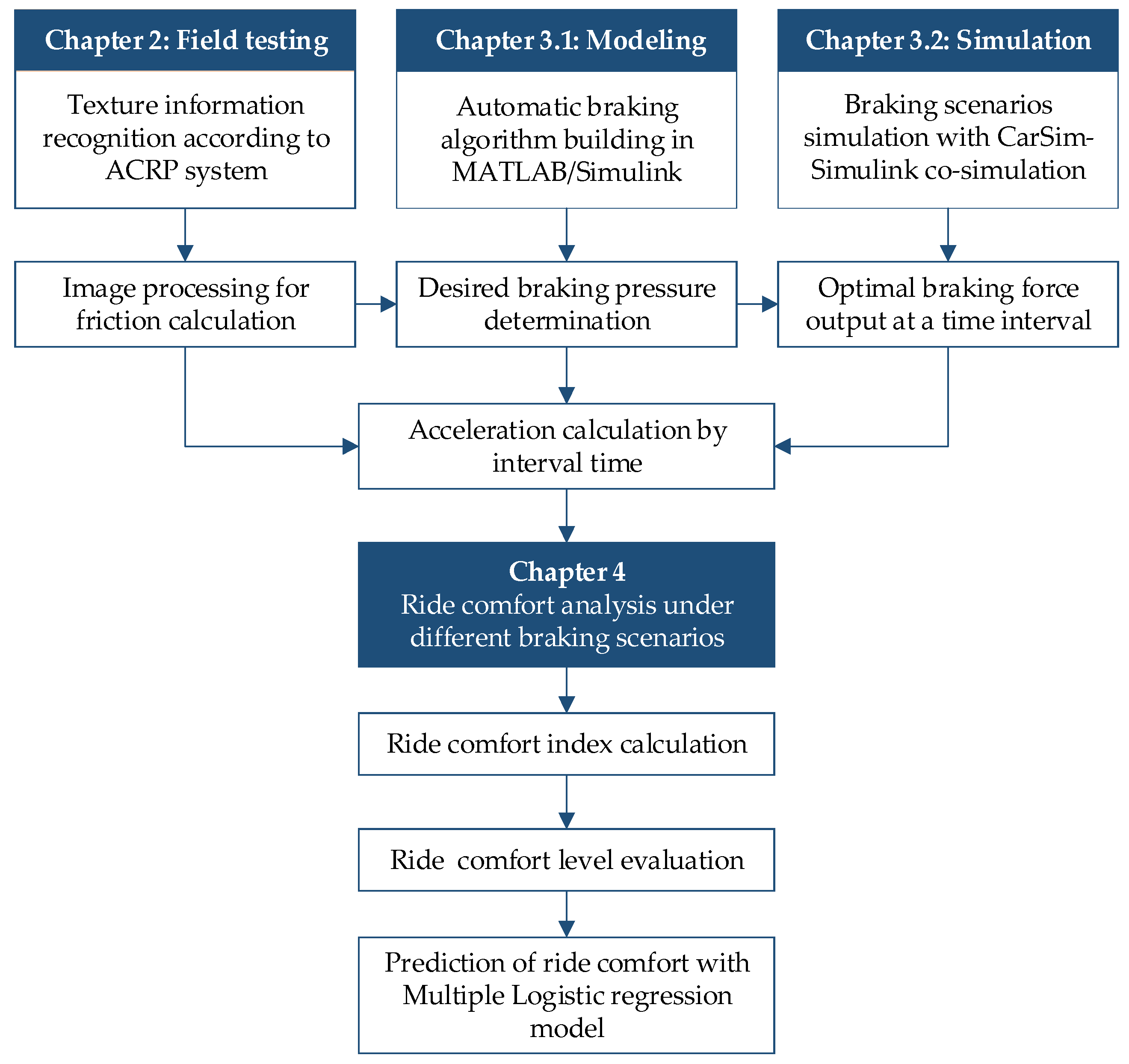
2. Field Testing

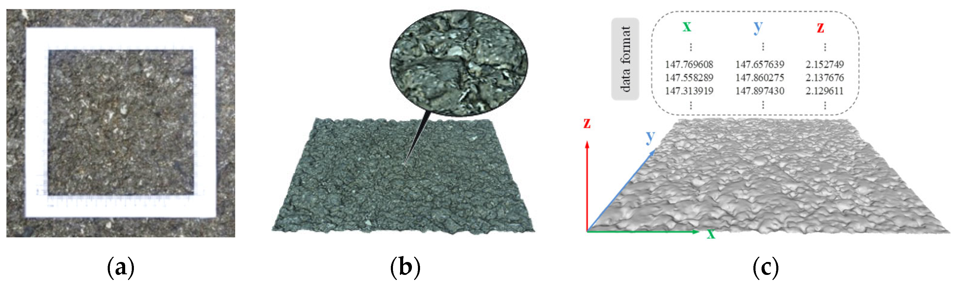
2.1. Field Testing of Road Surface Texture Information

Dense-graded asphalt concrete (AC-13) was selected in this study, and the gradation design of asphalt mixtures was shown in

Table 2. Gradations for AC asphalt pavement.

	Sieve Size (mm)	Passing Rate of Each Sieve (%)
Components		0.075	0.15	0.3	0.6	1.18	2.36	4.75	9.5	13.2	16
AC-13		6	10	13.5	19	26.5	37	53	76.5	95	100

. Then, the AC asphalt pavement (Figure 2a) had its surface textures captured on site using the research team’s automated close-range photogrammetry system (ACRP system) [32]. After preprocessing the gathered photos, the reverse reconstruction method was applied to rebuild the three-dimensional (3D) images of the surface texture of the asphalt pavement, and the 3D model of the surface texture of the asphalt pavement was constructed (Figure 2b). After preprocessing the reverse-reconstructed 3D model of the surface texture of the asphalt pavement with GeoMagic and MeshLab, it was possible to extract 3D elevation data for the surface texture of the road from the 3D model, which contained (x, y, z) 3D coordinate values (Figure 2c).

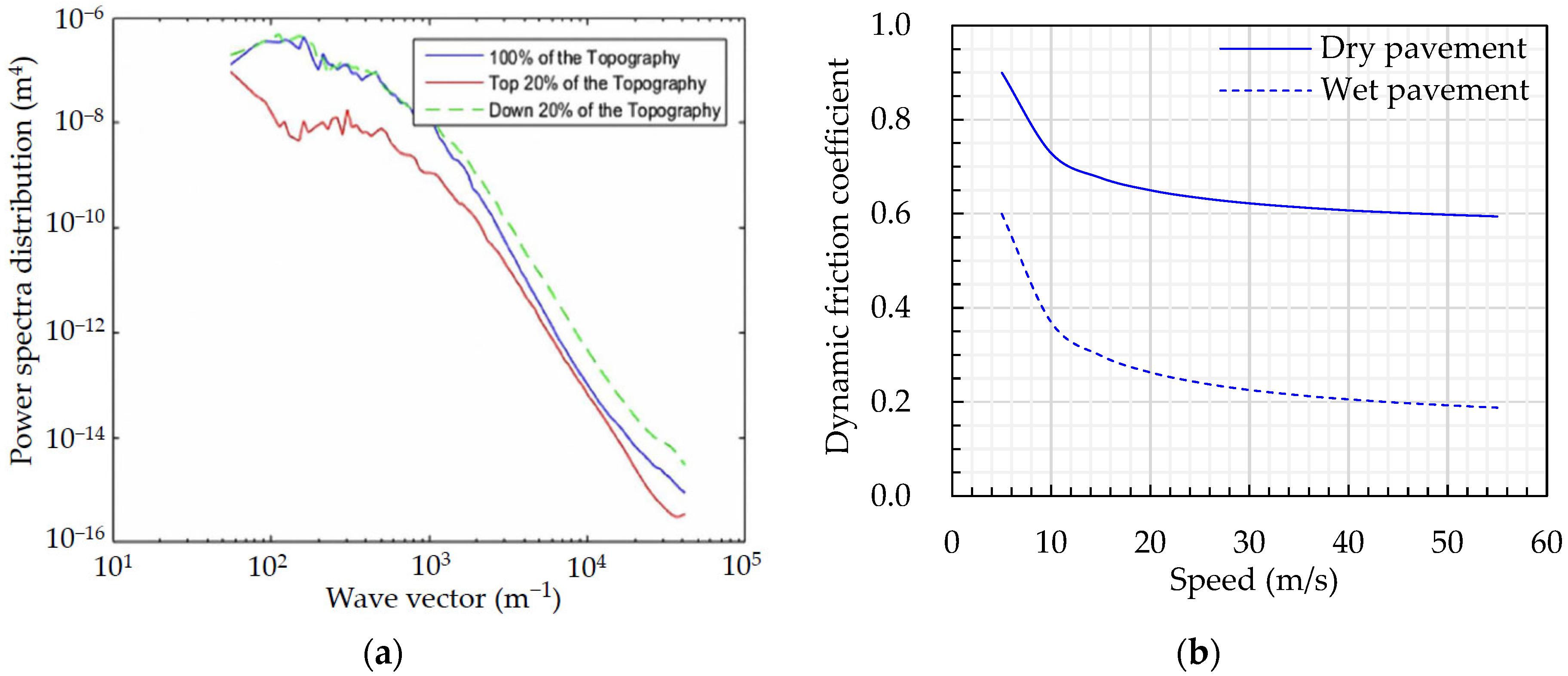
2.2. Calculation of the Dynamic Friction Coefficient

A power spectral distribution (PSD) solver was created in MATLAB using the PSD calculation model in the Persson friction theory and the 3D texture data (x, y, z) discussed in Section 2.1 [33,34,35]. Considering the random variables of the fractal road surface as discrete points, additional filtering, windowing and sampling window compensation of the coordinate values were required in the procedure of resolving the power spectrum [36].

In order to create a wet pavement surface, water was uniformly sprayed on the dry surface until the concave asperities were sealed with water [37,38]. The PSD of the wet and dry pavement surfaces were both calculated, as shown in Figure 3a.

$$C\left(q\right)=\frac{1}{{\left(2\pi \right)}^2}{\displaystyle \int 〈h\left(x\right)h\left(0\right)〉e^{iqx}}dx$$

(1)

where x is the wave vector direction; h(0) is the surface elevation of the origin point; h(x) is the surface elevation with the average elevation as the starting point; <...> represents the average across the plane; q is the wave vector, which could be obtained using the wavelength λ; and e is a universal constant.

In fact, when there is a water film on the road surface, the traditional method of calculating the PSD is not applicable, and the calculated road surface PSD is already inaccurate. This is because there is a water film barrier between the tire and the road, where the water film has a great lifting effect on the tire when the vehicle is driving at a high speed [39], and thus, there will be a larger untouched area between the vehicle tire rubber and the fractal surface of the asphalt pavement, which is one of the reasons for the significant decrease in the anti-skid performance of a vehicle during rainy weather.

The untouched area between the vehicle tire rubber and the fractal surface of the asphalt pavement is defined as the “anti-skid non-contribution area”. The asphalt pavement surface texture morphology and the “anti-skid non-contribution area” under dry and wet conditions were visualized, as shown in Figure 4. It can be seen that during the driving process in the wet condition, there is an unconnected area between the tire and the road due to the water stasis barrier and the water film lifting action, and these areas are called “anti-skid non-contribution areas”.

The friction coefficient curve, which was obtained using the Persson friction coefficient formula, varied with speed under different pavement conditions (dry and wet) (see Figure 2b). The curve tended to be gentler above 40 km/h, indicating that at relatively high speeds, the actual tire–road contact area stabilized. The friction coefficient of the wet state of the road surface was lower than that of the dry state, and the higher the speed, the greater the difference between the two states’ friction coefficients (dry and wet pavement).

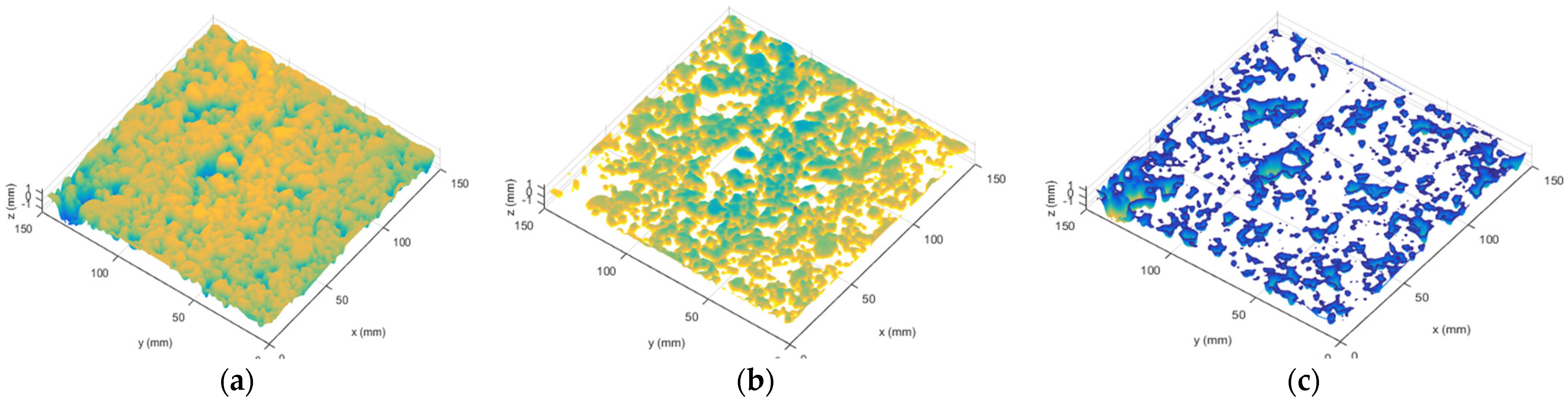
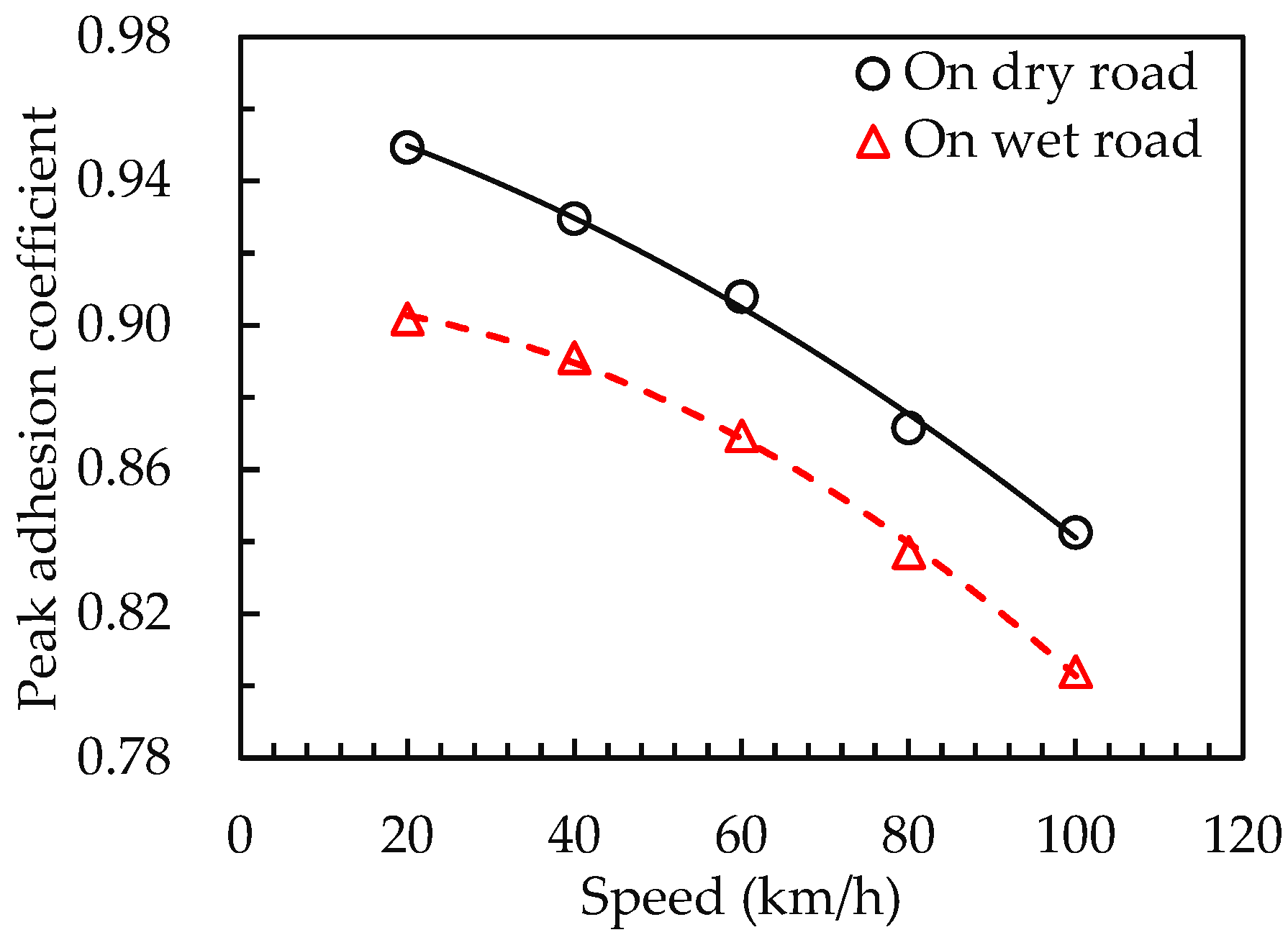
2.3. Peak adhesion Coefficient of the Asphalt Pavement

Referring to the tire hydroplaning model built by the research group [40,41], the dynamic friction coefficient curves (in Figure 3b) between the tire and pavement under various road conditions were integrated into the built hydroplaning model. We set the tire’s internal pressure to 240 kPa and the load to 3.922 kN. We also set the tire slip rate to approximately 15% and changed the rolling speed of the tire model while keeping other parameters constant. After that, the peak adhesion coefficient curve for various road conditions was determined, as shown in Figure 5.

The peak adhesion coefficient of the road surface gradually dropped with increasing vehicle speed, and the peak adhesion coefficient of the road surface was distributed as a convex parabola. The fundamental reason for this was that the tire’s rolling radius expanded at high speed, which increased the contact area between the tire and the road surface. Therefore, the adhesion force provided by the road surface was reduced. Obviously, the peak adhesion coefficient on a wet road was slightly lower than that on a dry road, which was mainly determined by the contribution rate of the road surface’s texture.

3. Braking Model

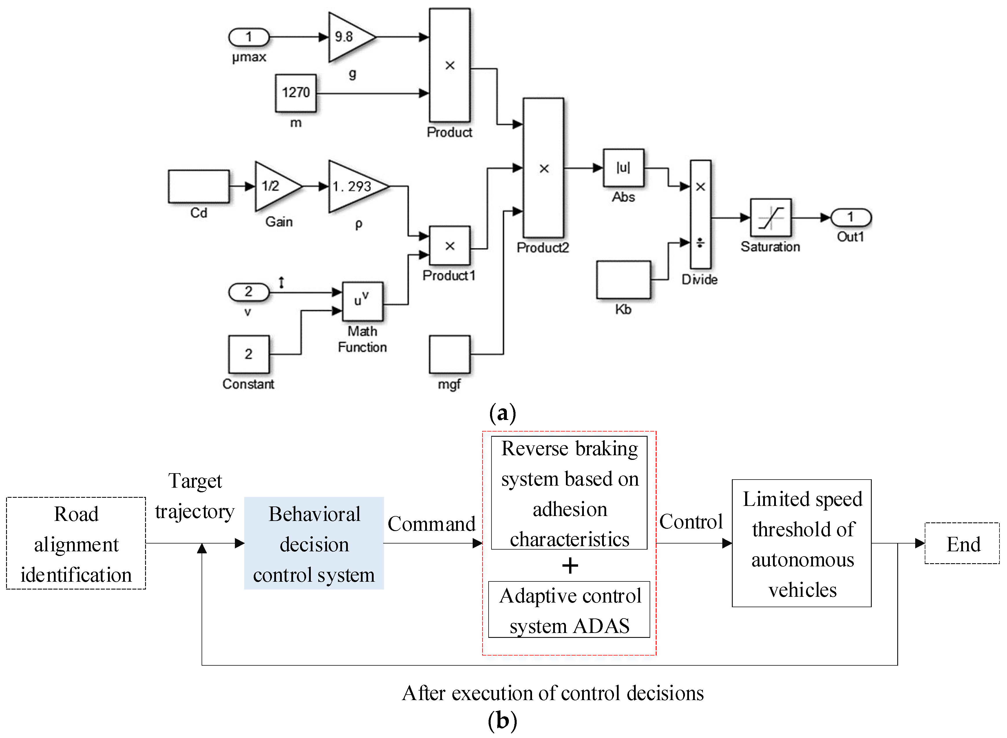
3.1. Braking Control Model

Based on the various peak adhesion coefficients of the road surface determined in real time, the appropriate braking deceleration was obtained. The required brake deceleration was converted into the desired brake pressure threshold by the anti-brake system model. Through the use of a brake pedal simulator, the electronic control unit (ECU) system of an AV determines the braking pressure. After determining the present brake situation, the brake actuator sends a brake signal to the pressure controller. To complete the vehicle’s autonomous braking procedure after a quick response, the brake system on the wheel sends the actual braking force to the tire in real time.

3.1.1. Braking Algorithm

The braking model of an AV was mainly adopted to calculate the wheel cylinder braking force under the condition of safe braking, that is, the calculation of the braking pressure P_des of the wheel cylinder. By considering driving straight on a road under good conditions, a mathematical model of forward braking dynamics was established. We set the vehicle deceleration behavior on a horizontal road in the model and ignored ramp resistance F_i. On this basis, air resistance and rolling resistance were considered. However, the slope resistance, a small amount of the acceleration resistance and the internal friction of the system were neglected [42]. Combined with Newton’s second law, the inverse braking model for an AV was obtained:

$$P_{des}=\frac{\left|m{a}_{des}+\frac{1}{2}{C}_{D}A\rho v^2+mgf\right|}{\left(T_{bf}+T_{br}\right)/r_r{P}_b}$$

(2)

where T_bf and T_br are the braking torques for the front and rear wheels, respectively; r_r is the tire rolling radius; and P_b represents the tire braking pressure.

According to the reverse braking model (Equation (2)) of an AV, the desired brake pressure P_des of the wheel cylinder was calculated. Then, the unit module of the reverse braking model was created in MATLAB/Simulink for the following CarSim/Simulink co-simulation, as shown in Figure 6a. The vehicle current speed v and pavement adhesion coefficient μ_h obtained above were integrated into the braking model. Regarding safety braking, the braking pressure P_des of the required wheel cylinder could be calculated in real time. The created braking model of an AV was integrated into CarSim to replace the original braking model of a conventional vehicle.

In order to make the automatic steering behavior of an AV closer to the driver’s operability, the adaptive braking control approach was implemented by the system to alter the state of the vehicle in real time, which ensured that the vehicle would pass through the curved section at the optimal speed along the optimal travel path (in Figure 6b). During the steering process, the car drove at the ideal speed limit to ensure braking comfort and safety. Under the optimized state of the permitted lateral offset distance, the car drove off the curve with the shortest braking time to achieve the best braking effect according to the ideal braking force based on road surface adhesion characteristics. The steering system calculated the driving speed in real time to avoid exceeding the speed limit so that the autonomous vehicle ran along the intended path.

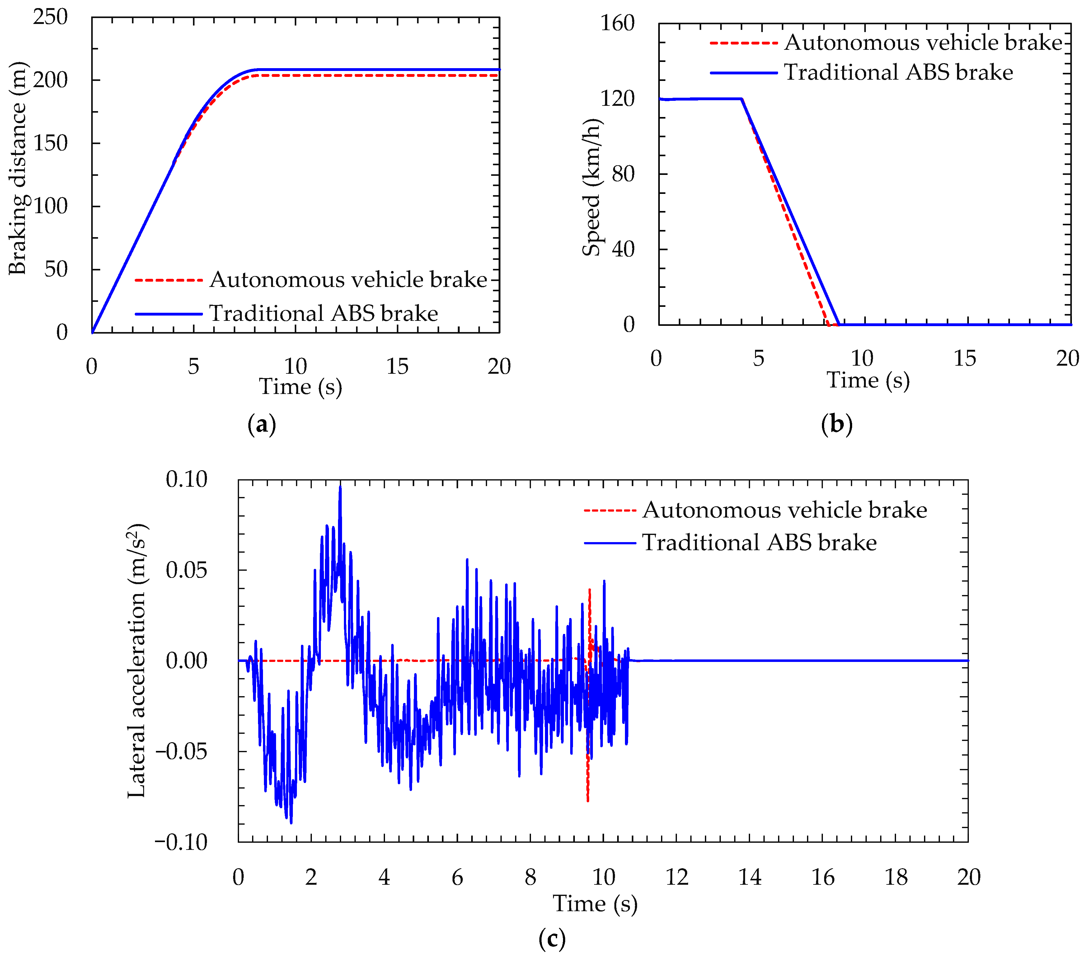
3.1.2. Validation of the Braking Model

Simulink was used to build a model of the brake control algorithm based on the proposed brake system for the AV. The precision of the brake system in comparison to the conventional ABS brake system was then validated through co-simulation using CarSim. An excellent road condition was used in the simulation, and a peak adhesion coefficient of 0.90 was chosen for the AC-13 asphalt pavement in a dry state. The initial driving speed was set to 120 km/h at the start of braking, the throttle percentage was 0 degrees and the simulation time step was 20 s.

The conventional ABS braking vehicle was subjected to a constant braking pressure of 10 MPa in order to reflect its maximum braking effectiveness. The autonomous car used an adaptive braking control system to brake with the anticipated braking force depending on the characteristics of the adhesion of the road surface. The braking performance curves of the vehicle under two scenarios were determined using the simulation results and are displayed in Figure 7a,b. It is clear that the autonomous vehicle’s braking performance surpassed that of the conventional ABS. The braking distance was decreased by 10.92 percent, while the braking time was lowered by 10.95 percent. It can be observed from a comparison of the lateral acceleration–time curves for the two scenarios (in Figure 7c) that the autonomous car had roughly consistent lateral acceleration while braking, whereas a standard ABS vehicle had variable lateral acceleration.

The traditional ABS frequently switched between solenoid valves during the braking process to maintain the tire slip rate within the ideal range of 10–20%. As a result, the tire slip rate fluctuated more frequently without consideration of the road characteristics, which led to extremely poor braking performance and a bad passenger experience. Based on the road adhesion characteristics, the braking system of the autonomous vehicle calculated the expected braking pressure at the real-time position and applied it to the tires so that the vehicle drove with the optimal braking deceleration. The tire slip rate of the autonomous vehicle was basically maintained at approximately 12.0% and the fluctuation range was very small.

When the actual tire–road contact characteristics are taken into account in the braking system of an AV, it can better reflect the vehicle braking stability requirements. It was found that the braking system performance of the AV outperformed traditional ABS. The results showed that the proposed braking system is suitable for AVs and has high accuracy.

In accordance with the aforementioned created autonomous vehicle model and pavement model, the simulation analysis under various operating conditions was carried out in CarSim. Meanwhile, the model written in MATLAB/Simulink was integrated into CarSim to replace the original braking model (in Figure 8). In this study, the braking scenarios of emergency braking and braking on curved and slope sections were analyzed in wet or dry road conditions.

3.2. Modeling Parameter Settings

(1) Travel path modeling

The reference path, pavement geometry and pavement roughness attributes are key elements of the pavement model in a simulation. As illustrated in Figure 9, the segmentation approach was used to input the pavement’s linear key points coordinate data, converting the created reference path into (x, y) coordinates to lessen the workload associated with data entry. The pavement geometry properties (road width, number of lanes, elevation, etc.) were mapped to the matching (x, y) coordinates in the CarSim pavement model database. The adhesion coefficient of the continuous point on the road surface, which was acquired in real time, was also imported.

(2) Vehicle parameters

We selected the common SUV type used in a city as the simulation vehicle model; the vehicle body parameters are shown in

Table 3. Parameter settings of the vehicle body.

Items	Value	Items	Values
Vehicle mass	2257 kg	Distance between the centroid and front axis	1330 mm
Vehicle length	4475 mm	Axle spacing	3140 mm
Vehicle width	2029 mm	Roll inertia Ixx	846.6 kg·m2
Vehicle height	1966 mm	Pitch inertia Iyy	3524.9 kg·m2
Centroid height	780 mm	Yaw inertia Izz	3524.9 kg·m2

. The specific aerodynamic parameters were set in the simulation, including the vehicle’s windward surface area (the SUV vehicle was taken to have an area of 3.3 m²) and air density (taken as 1.206 kg/m³). The vehicle tires acted as the only contact parts between the vehicle and the pavement. Theoretically, the force generated from the tire–road interaction ensures the braking safety of the vehicle. To make the vehicle simulation analysis comparable to a real-world situation, the adhesion characteristic curve for the tire–road interaction calculated by our research group was imported into CarSim [43].

Due to the large difference between the autonomous vehicle and the traditional manned vehicle in terms of the braking system, an algorithm for an autonomous vehicle braking model was written using Matlab/Simulink co-simulation to ensure the simulation accuracy. Then, the written model was imported into CarSim to replace the initial braking model.

(3) Sensing parameter settings

The AEB (autonomous emergency brake) system of the autonomous vehicle was simulated. The POP UP Windows subroutine was created using the CarSim interface to display the car driving data using MATLAB. The engine speed, vehicle speed, throttle position and brake percentage were among the selectable statistics. Additionally, the effective maximum brake pressure of the wheel cylinder was divided by the present brake pressure to get the braking percentage. Figure 10a displays a dynamic visualization of the simulation findings.

In the simulation, a short-range laser radar was utilized to detect automobiles and pedestrians in proximity to the vehicle, and the long-range laser radar was customized to detect the traffic situation in the distance. The two radars’ respective effective ranges were 150 m and 30 m, and their horizontal viewing angles were 9 deg and 80 deg. Additionally, Figure 10b illustrates that both of the two radars’ vertical viewing angles were 9 deg.

4. Braking Scenario Simulations

4.1. Emergency Braking on a Straight Road

If an autonomous vehicle is in an emergency during the driving process, in order to avoid a collision, it is necessary to trigger the brake as soon as the vehicle sensor recognizes the danger. Then, the braking force is continuously exerted on the wheel cylinder to stop the vehicle as soon as possible. In the case of emergency braking, only considering safety without passenger comfort, a 500 m long straight road was built in the simulation.

First, the braking effect of an SUV traveling at a speed of 120 km/h on a rainy day was tested. The friction coefficient curve of the road surface calculated using the PSD power spectral density of “anti-skid non-contribution area for skid resistance” on a rainy day was imported. The obstacle ahead was set to be detected in the fourth second. Meanwhile, the vehicle started emergency braking. At the beginning of the fourth second, a braking pressure of 10 MPa was applied instantaneously, as shown in Figure 11.

The vertical force of the front wheel rose suddenly while that of the rear wheel fell suddenly. Meanwhile, the car body leaned forward. When the braking pressure was applied instantaneously, the tires were quickly locked and then began to skid. Then, the ABS of the vehicle began to operate and the vertical force curves of the wheels began to oscillate repeatedly. Similarly, the simulation results with different braking pressure settings of 8 MPa, 6 MPa, 4 MPa, 2 MPa, 1 MPa and 0.5 MPa were also calculated.

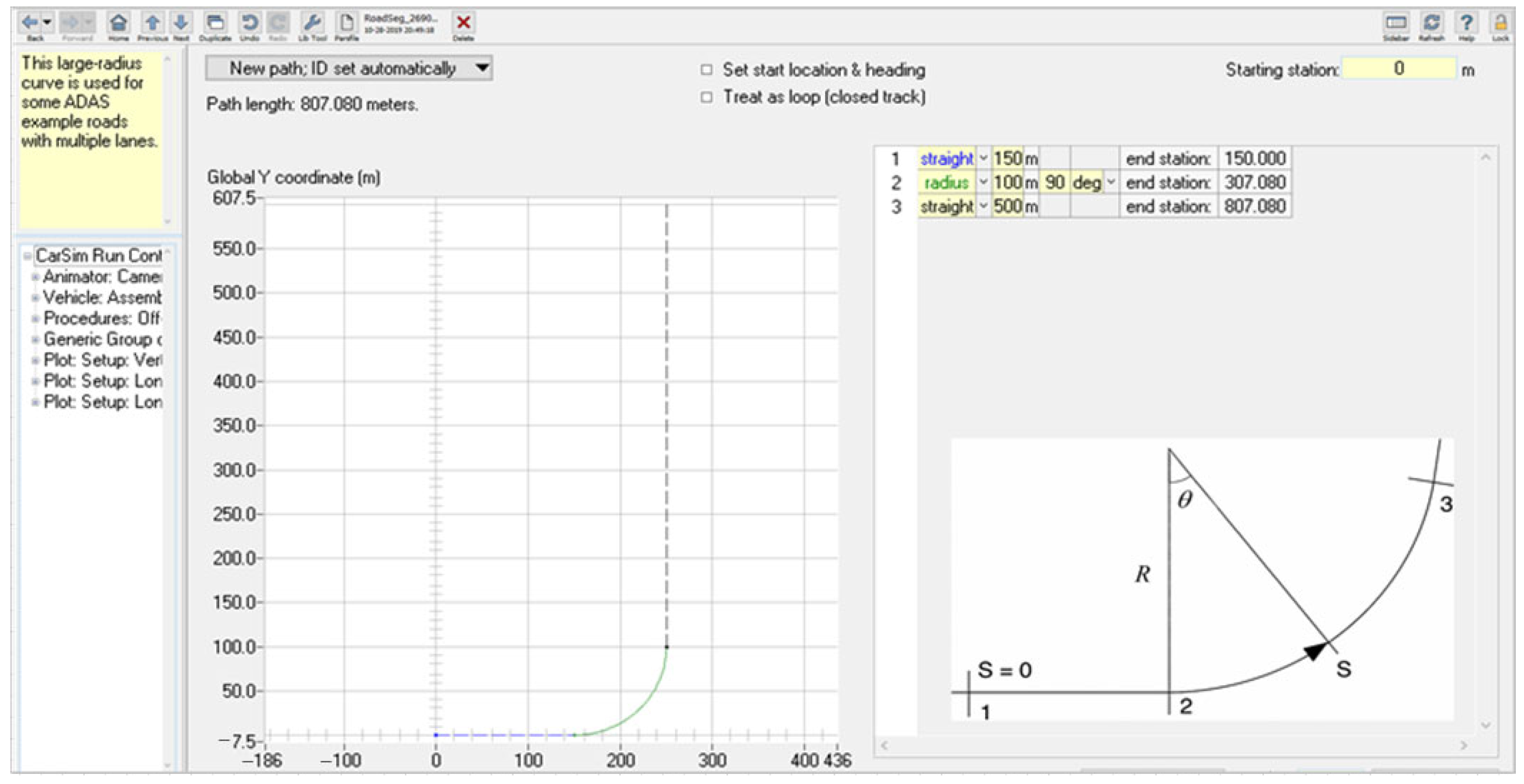
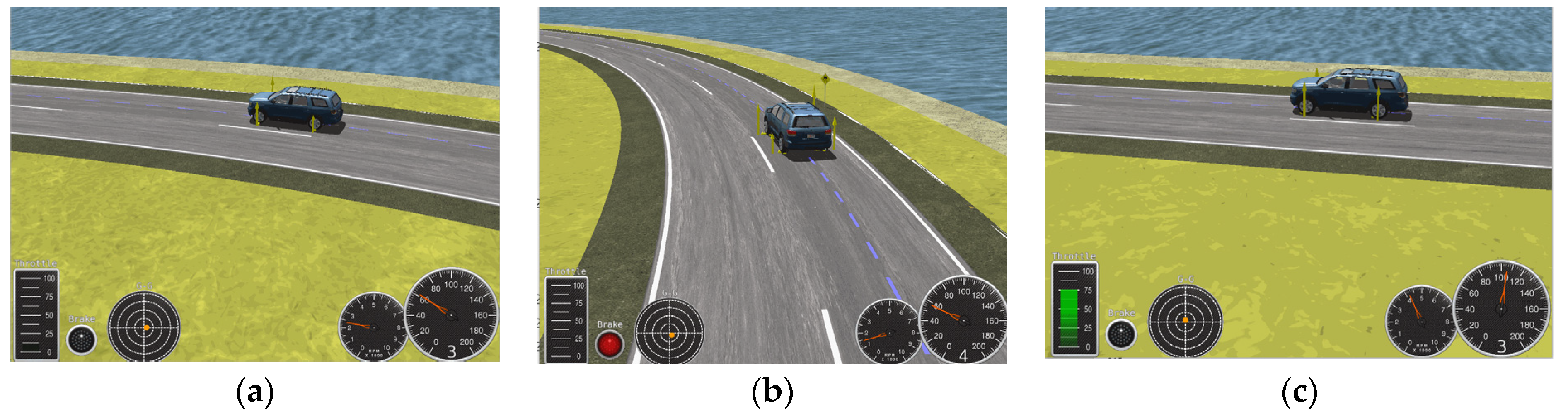
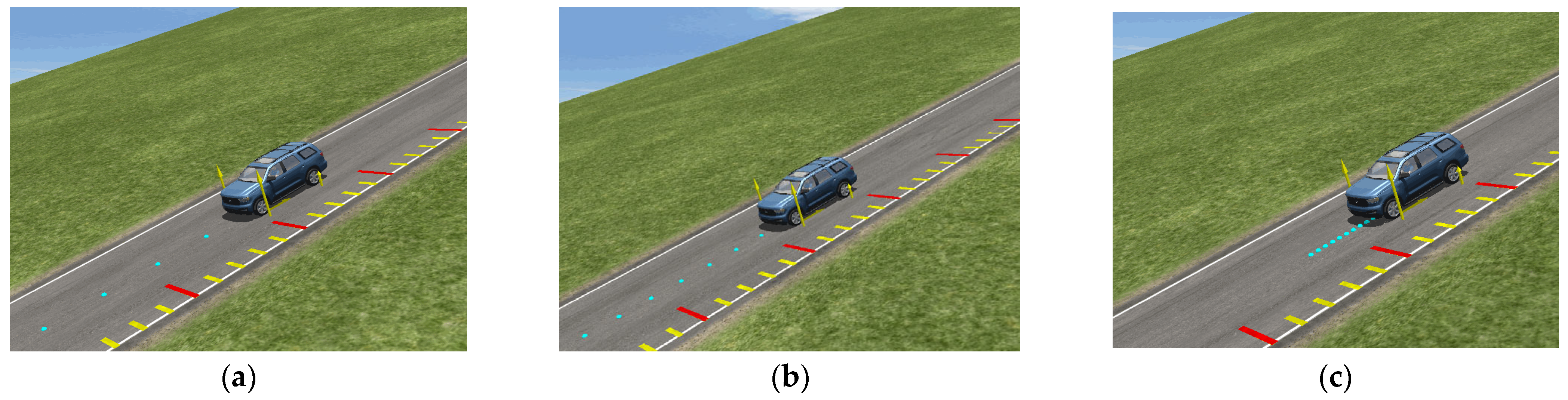
4.2. Steering Braking on a Curved Section

In the simulation, a 700 m long road with both straight and curved sections was constructed. A 30 s simulation time was chosen. On both sides of the fictitious road, there were signs indicating the speed limit, safety precautions and lane changes. The model car initially moved at a constant speed of 100 km/h. In addition, the vehicle received a long-range radar, camera and other sensors at the same time. The car could dynamically identify the road surroundings while driving with sensors installed.

The road was identified by the sensors, and an automatic optimal cornering speed was implemented to modify the brake cylinder pressure in real time. At the same time, the lateral acceleration was not more than 0.35 g to ensure the stability of the vehicle when turning. The braking simulation visual interface is shown in Figure 12. Additionally, the adhesion coefficients for wet and dry roads were set to 0.60 and 0.90, respectively.

4.3. Braking Simulation on a Sloped Road

It is well known that there is frequent braking when driving uphill and downhill. The vehicle brake can easily fail and there is a blind spot in the onboard camera. In order to maintain a sufficient safety distance and braking comfort, the autonomous vehicle must maintain enough distance in front before starting braking. Braking characteristics on a sloped road were analyzed by considering passenger comfort during the vehicle braking process in this study.

Based on the vehicle dynamics model mentioned above, four slope gradients (5°, 10°, 15° and 20°) were selected in the simulation, taking the dry road condition with good skid resistance as an example (the pavement peak adhesion coefficient was taken as 0.8065). Keeping the other parameters constant, the scene visualization of braking on a sloped road was obtained, as shown in Figure 13.

5. Results and Discussion

5.1. Evaluation Index of the Braking Comfort

The comfort index (CI) of AVs is specified in International Standard ISO 2631-1 [44]. Without considering the lateral movement, the calculation equation of the comfort index can be simplified to

$$CI={\left[\frac{1}{m}{\displaystyle \sum _{i=0}^m{a}_i^2}\right]}^{1/2}$$

(3)

where a_i is the ith statistically determined acceleration value and m is the total number of statistics. In successive simulation trials, the acceleration values were measured at equal time intervals (Δt = 1 s), which is consistent with the statistical frequency of comfort (within 0.5 Hz~80.0 Hz). Six comfort levels were defined in accordance with the comfort index’s range and the International Standard ISO 2631-1, as shown in

Table 4. Comfort evaluation level for autonomous vehicle braking.

Levels	CI Range (m/s2)	Description of Vehicle Comfort	Color
0	>2.0000	Extremely uncomfortable
1	1.2500~2.5000	Very uncomfortable
2	0.8000~1.6000	Uncomfortable
3	0.5000~1.0000	Fairly uncomfortable
4	0.3150~0.6300	A little uncomfortable
5	<0.5000	Comfortable

. The comfort of operating a vehicle lies between two comfort levels when the CI level ranges overlap.

5.1.1. Calculation of Braking Comfort Index

On a dry or wet road, the speed–time relationship was obtained according to the simulation results. Then, the ride comfort level was evaluated for each different braking scenarios according to Equation (3) and Table 4. Taking emergency braking on a straight road as an example, the simulation results are as follows.

The calculation results of the comfort index of the autonomous vehicle during the emergency braking process on dry and wet road conditions are shown in

Table 5. Comfort level of emergency braking on a dry road.

Time Interval (s)	Comfort Index CIP with Different Braking Pressures (m/s2)
	CI0.5	CI1.0	CI2.0	CI4.0	CI6.0	CI8.0	CI10.0
Δt1	5	5	5	5	5	5	5
Δt2	5	5	5	5	5	5	5
Δt3	5	5	5	5	5	5	5
Δt4	5	5	5	5	5	5	5
Δt5	5	4	3	2	1~2	1~2	1~2
Δt6	5	4	3	2	1~2	1~2	1~2
Δt7	5	4	3	2	1~2	1~2	1~2
Δt8	5	4	3~4	2	1~2	1~2	1~2
Δt9	5	4	3~4	2	5	5	5
Δt10	5	4	5	5	5	5	5
Δt11	5	4	3~4	5	5	5	5
Δt12	5	4	3~4	5	5	5	5
Δt13	5	4	3~4	5	5	5	5
Δt14	5	4	4	5	5	5	5
Δt15	5	4	5	5	5	5	5
Δt16	5	4	5	5	5	5	5
Δt17	5	4	5	5	5	5	5
Δt18	5	4	5	5	5	5	5
Δt19	5	4	5	5	5	5	5
Δt20	5	5	5	5	5	5	5
Δt21	5	5	5	5	5	5	5

and

Table 6. Comfort level of emergency braking on a wet road.

Time Interval (s)	Comfort Index CIP with Different Braking Pressure (m/s2)
	CI0.5	CI1.0	CI2.0	CI4.0	CI6.0	CI8.0	CI10.0
Δt1	5	5	5	5	5	5	5
Δt2	5	5	5	5	5	5	5
Δt3	5	5	5	5	5	5	5
Δt4	5	5	5	5	5	5	5
Δt5	5	4	3	2	2	2	2
Δt6	5	4	3	2	2	2	2
Δt7	5	4	3	2	2	2	2
Δt8	5	4	3~4	2	2	2	2
Δt9	5	4	3~4	2	2	2	2
Δt10	5	4	3	2	2	2	2
Δt11	5	4	3~4	5	5	5	5
Δt12	5	4	3~4	5	5	5	5
Δt13	5	4	3~4	5	5	5	5
Δt14	5	4	4	5	5	5	5
Δt15	5	4	5	5	5	5	5
Δt16	5	4	5	5	5	5	5
Δt17	5	4	5	5	5	5	5
Δt18	5	4	5	5	5	5	5
Δt19	5	4	5	5	5	5	5
Δt20	5	4	5	5	5	5	5
Δt21	5	4	5	5	5	5	5

.

5.1.2. Evaluation of Ride Comfort Levels

(1) Emergency Braking on a Straight Road

From Table 4 and Table 5, when the braking pressure was 0.5 MPa or 1.0 MPa, the ride comfort was always in a good state within a specific braking time range (ΔT = 20 s), and the comfort level was always 5 or 4. However, the vehicle braking behavior was not completed at the end of 20 s, and its braking comfort was subsequently not evaluated. As the brake pressure changed from 2 MPa to 10 MPa, the following was found:

• The comfort index CI of an autonomous vehicle on a dry road during the period of constant speed (in the time domain of Δt₁~Δt₄) was within the range of 0–0.315, indicating that straight travel at a certain safe speed with real-time perception of the surrounding environment produced ride comfort that was suitable for the passenger’s subjective feelings and provided a good riding experience. Due to the low coefficient of adhesion on the wet road, the braking time of the vehicle under the same braking pressure and same initial speed increased, and the braking distance increased in turn. Compared with the dry road condition, braking comfort was poor and the passengers were prone to fatigue.
• When the braking pressure was 2 MPa, the braking time was extended in the case of an initial speed of 120 km/h. During the period of 5–19 s, the comfort level was 4, meaning that the passengers felt slightly uncomfortable but the comfort was within an acceptable range. However, the longer braking time caused the ABS to start frequently and cause passenger fatigue, and there was a high probability of collision and rear-end collision in the emergency braking environment.
• When the braking pressure changed from 4 MPa to 10 MPa, the comfort level was 5 during the constant speed driving phase. During the brake deceleration process, the comfort level appeared in the range of level 2 (brake pressure was equal to 4 MPa) or level 1~level 2 (brake pressure was more than 4 MPa), indicating that the vibration frequency of the vehicle during braking was large, and the uneven distribution of the vertical pressure of the left and right tires resulted in a large fluctuation.

(2) Steering braking on a curved section

As for the sections with different curve radii, the evaluation of ride comfort level in dry and wet road conditions was carried out. The following was found:

• The best curve radius in terms of comfort was 200 m at a speed of 100 km/h, and the CI index was less than 4. This meant that the comfort met the passenger requirement, and the advantage of the AV was demonstrated.
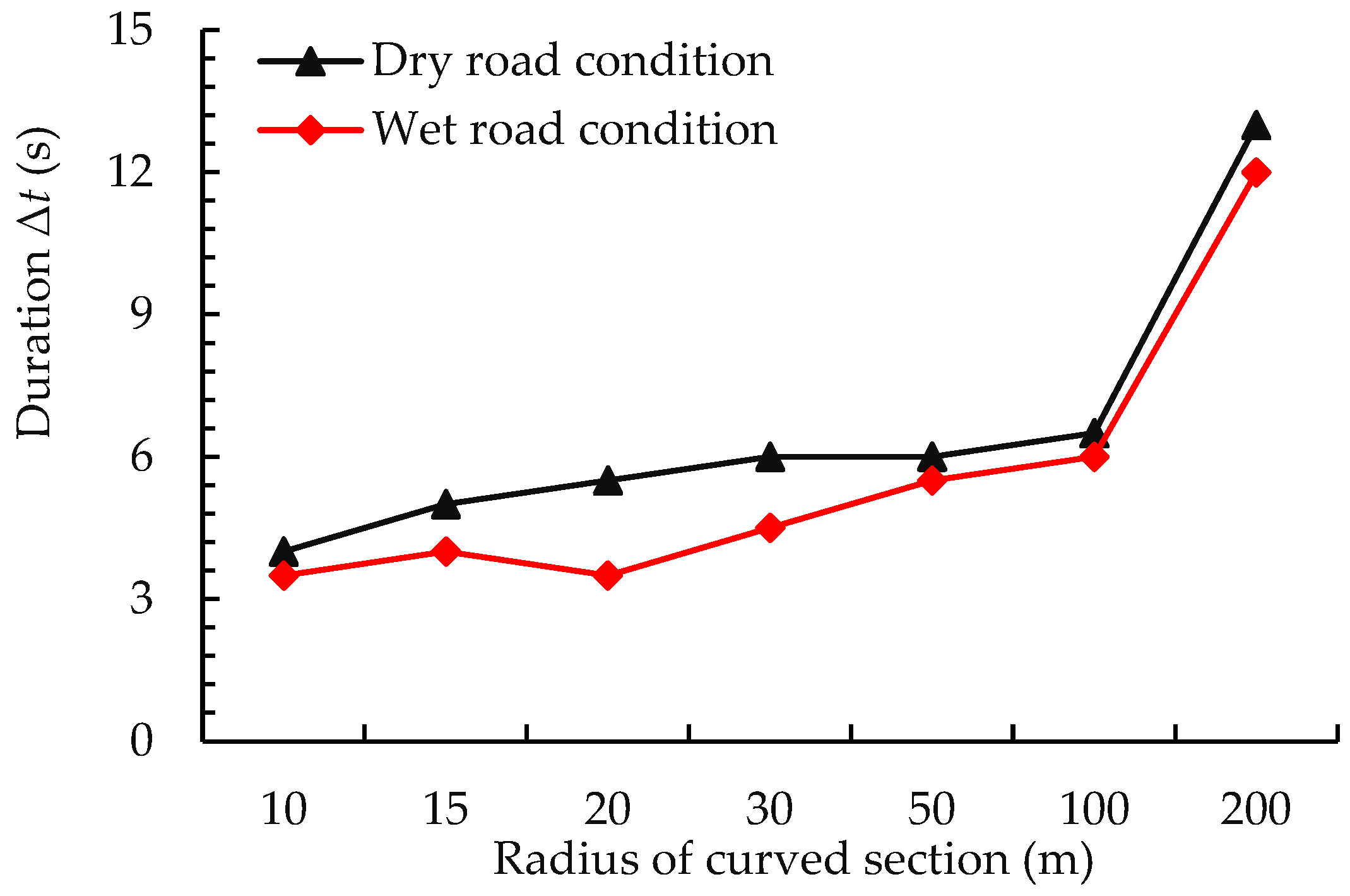
• Compared with the wet road condition, a dry road could provide greater lateral friction because of the good adhesion, which mostly counteracted the centrifugal force generated by the vehicle on the curved section. Thus, the ride comfort during the steering process was greatly improved, and thus, the duration of the “curve balance state” on the dry road lasted longer, i.e., an increase of approximately 57.14% compared with the wet road condition, as shown in Figure 14. In addition, the “curve balance state” was defined as the duration of ride comfort level 5 during the steering braking process.
• As the radius of the curve increased, the braking comfort of the vehicle during cornering was relatively good. This was because the curve length increased with the increased radius of the curved section. The autonomous vehicle used an adaptive control system to navigate the curved segment at the best speed; for curves with a bigger radius, a speed buffering process was in place. Road alignment design might be based on the comfort evaluation results.

From Figure 14, the “curve balance state” duration slightly increased with the radius increase when the curve radius R was ≤100 m, but the variation was not significant. When the radius R was >100 m, the “curve balance state” duration increased significantly. This shows that the curve radius was a significant factor that influenced the ride comfort of AVs during the steering braking process. In order to improve the ride comfort of the vehicle, it is recommended that the curve radius R should be ≥100 m and the brake deceleration should start at least 100 m from the entrance of the curved section.

According to Figure 13, when the curve radius R was ≤100 m, the “curve balancing state” duration increased somewhat with the radius increase, but the difference was not statistically significant. The “curve balance state” time greatly increased when the radius R was >100 m. This demonstrated how the curve radius had a big impact on how comfortable an AV will ride when steering and stopping. It is advised that the curve radius R should be ≥100 m and the brake deceleration should commence at least 100 m from the beginning of the curved segment in order to increase the ride comfort of the vehicle.

(3) Braking on a sloped road

According to the simulation results of the comfort level under different braking speeds and slope gradients, the change law of vehicle comfort was analyzed. The following was found:

• When the slope gradient i = 10° and the initial speed was 80 km/h, or when the slope gradient i = 20° and the initial speed was 60 km/h, the ride comfort level was not greater than 3, indicating that the road slope gradient had a significant effect on the initial braking speed and comfort level. Compared with the slope gradient of 10°, the ride comfort was poor for a slope with a gradient of 20°, which was consistent with the vehicle braking dynamics characteristics.
• Under the conditions of a small slope gradient and low initial speed (such as i = 10° and v₀ = 60 km/h) or a large slope gradient and high initial speed (such as i = 20° and v₀ = 80 km/h), after perceiving obstacles ahead, because the frictional force on the road surface was insufficient to counteract the inertial force generated by the vehicle body mass, the vehicle started to drive at a uniform acceleration (a = g*sin(i)). Then, the safe braking distance was sensed dynamically and the automatic control mode was activated to adjust the wheel cylinder pressure. Braking deceleration started at the fifth second. In order to prevent the vehicle from rolling over on the sloped road, the vertical pressures of the front and rear tires were automatically controlled to achieve a stable state. At this stage, the vehicle generated a large vibration frequency, and thus, the comfort was poor, with an evaluation level of 2.0.
• As the vehicle mass and the position of the mass center were the same, the braking process on a slope mainly depended on the comprehensive effect of the slope and the initial speed. In a similar braking environment, an AV needs to automatically adjust the wheel cylinder braking pressure according to the initial speed and road slope gradient to adapt to the road alignment to achieve a safe braking behavior.

5.2. Prediction of the Ride Comfort

5.2.1. Multiple Logistic Regression Model

A logistic regression model was used to study the relationship between multiple independent and dependent variables and establish a probabilistic prediction model for discrimination or classification. Logistic regression models are used in a wide range of fields, including machine learning, most medical fields [45] and the social sciences [46]. For a logistic regression model, the most prominent advantage is its simplicity and strong interpretability [47,48].

In order to fit the actual probability of occurrence, there must be a correlation between the selected independent variable and the dependent variable, and each variable is mutually exclusive. Compared with multiple linear regression, logistic regression analysis has the advantages of requiring a low number of assumptions and having a high model accuracy. Therefore, a logistic regression model was applied to build the comfort prediction model of the AV. First, a single-factor analysis was performed for each variable. On this basis, the factors with statistical significance were selected for multivariate unconditional logistic regression analysis, and the optimal model was obtained using the stepwise regression method [49].

Based on the variation range of comfort levels (from level 1 to level 5) under different braking scenarios in Section 5.1.2, level 5 as the highest dependent variable result was selected as the reference group, and the braking comfort of the AV was regarded as a binary dependent variable y_i, where y_i = 0 represented level 5 and y_i = 1 represented level 1~level 4. In addition, each independent variable X = (X₁, X₂, …, X_n) was regarded as a quantitative or qualitative variable in the logistic regression model, which was applicable to both continuous and discrete variables [50]. Thereby, the probability P(Y_i) that the i^th comfort level occurred was denoted as P_i:

$$P_i=P\left(y_i=1\left|X_1,X_2,\dots ,X_n\right.\right)$$

(4)

The expression of the binary logistic regression model was as follows:

$$\log it\left(P_i\right)=\ln \left(\frac{P_i}{1-P_i}\right)=\alpha +{\beta }_1{X}_{1i}+\dots +{\beta }_n{X}_{ni}$$

(5)

Then, the probability for different comfort levels was

$$P_i=\frac{\exp \left(\alpha +{\beta }_1{X}_{1i}+\dots +{\beta }_n{X}_{ni}\right)}{1+\exp \left(\alpha +{\beta }_1{X}_{1i}+\dots +{\beta }_n{X}_{ni}\right)}$$

(6)

where α is a constant and the β_i are the regression coefficients representing the correlation between the independent and dependent variables. In addition, P_i/(1 − P_i) = exp(β) is the odds ratio or the relative risk, which is an important index to measure the influence degree of the independent variable on the dependent variable. For each additional unit of the independent variable, the probability of a certain comfort level of the dependent variable will increase by exp(β_i) units.

In this study, the Hosmer–Lemesshow was used to test whether the theoretical frequency distribution predicted by the logistic regression model conformed to the actual theoretical frequency distribution. In addition, the model was globally tested according to the conditional parameter likelihood ratio test and non-significant variables were excluded.

5.2.2. Prediction Model of the Ride Comfort

Based on Section 5.2, the discrete comfort index of each time interval (Δt = 1.0 s) under different braking pressures was acquired. In addition, the braking pressure (X_1i) and time (X_2i) were the only considered independent variables. Obviously, the tire force during the braking process showed a strong nonlinear characteristic. The binary classification logistic regression analysis was applied to obtain the prediction model of ride comfort for the AV on a straight road during an emergency braking process, which can be expressed as

$$\log it\left(P_j\right)=f\left(P,\Delta t,k_1\right)$$

(7)

where P_j is the probability of the jth comfort level (j represents the four levels of ride comfort, that is level 1~level 4), P is the vehicle braking pressure, Δt is the time interval of acceleration acquisition during the vehicle braking process, and k₁ is the influence coefficient related to the sensor and vehicle type.

The multiple logistic regression model was applied to predict the probability of different ride comfort levels. The regression analysis results are shown in

Table 7. Results of the logistic regression analysis on a dry road.

Prediction Model		Regression Coefficient	Standard Error	t	PL > |t|	95% Confidence Interval
Level 2	Constant	−1.5291	0.6514	−2.35	0.019	−2.8060~−0.2523
	P	0.2545	0.0835	3.05	0.002	0.0909~0.4181
	Δt	−0.1429	0.4649	−3.07	0.002	−0.2341~−0.0518
Level 3	Constant	−0.7336	0.8356	−0.88	0.038	−2.3713~−0.9041
	P	−0.3676	0.2001	−1.84	0.015	−0.0542~0.3509
	Δt	−0.0722	0.0708	−1.02	0.031	−0.2110~0.0667
Level 4	Constant	−0.3744	0.7033	−0.53	0.029	−1.7528~1.0039
	P	−0.8316	0.2528	−3.29	0.001	−1.3270~−0.3362
	Δt	0.0571	0.0479	1.19	0.023	−0.0368~0.1510

. Among them, the t-test was the significance test of a single independent variable. The constants and the significance level PL of the independent variables were less than 0.05, indicating that the coefficient of each variable was significant as shown in

Table 8. Hausman test result of the prediction model.

Model	Test Coefficient chi2	df	Snell R-Squared	PL > chi2	Significance
Level 2	−2.561	6	0.2209	1.000	For Ho
Level 3	−2.376	6		1.000	For Ho
Level 4	−1.503	6		1.000	For Ho
Level 5	14.951	3		0.002	Against Ho

Note: d_f is the number of degrees of freedom.

.

According to the regression analysis results in Table 5, the comfort evaluation model of the AV during emergency braking on a straight road under a dry road condition was obtained as follows:

$$\begin{array}{l}\log it{P}_{j=\mathrm{Level}2}=-1.5291+0.2545P_i-0.1429\Delta t_i\\ \log it{P}_{j=\mathrm{Level}3}=-0.7336-0.3676P_i-0.0722\Delta t_i\\ \log it{P}_{j=\mathrm{Level}4}=-0.3744-0.8316P_i+0.0571\Delta t_i\end{array}$$

(8)

Based on Equation (8), it can be seen that the influence of braking pressure on ride comfort in the level 2 model showed a linear growth trend, while the level 3 and level 4 models showed non-linear decreasing trends with increasing braking pressure. Theoretically, when the brake pressure is too high, the vertical pressure of the tire will be generated instantly, which makes passengers feel highly uncomfortable. However, if the braking pressure is too small to complete the braking process within the effective time, this inevitably leads to a collision and a rear-end accident. Therefore, it is suggested that the braking pressure should be controlled to within the range of 4~6 MPa. Considering the comfort and safety during the vehicle braking process, the braking pressure on a wet road should be within 3~4 MPa. Similarly, the prediction models under other braking scenarios were also obtained as follows:

• Emergency braking on a wet road:

$$\begin{array}{l}\log it{P}_{j=\mathrm{Level}1}=-3.5729+0.3758P_i-0.2051\Delta t_i\\ \log it{P}_{j=\mathrm{Level}2}=-1.6798+0.1484P_i-0.1522\Delta t_i\\ \log it{P}_{j=\mathrm{Level}3}=-0.8187-0.3722P_i-0.0872\Delta t_i\\ \log it{P}_{j=\mathrm{Level}4}=-0.1853-0.7846P_i+0.0198\Delta t_i\end{array}$$

(9)

• Steering braking on a curved section:

  (a)

  On a dry road:

  $$\begin{array}{l}\log it{P}_{j=\mathrm{Level}3}=1.1966-0.0203R_i-0.1391\Delta t_i\\ \log it{P}_{j=\mathrm{Level}4}=0.7108-0.0070R_i-0.1115\Delta t_i\end{array}$$

  (10)

  (b)

  On a wet road:

$$\begin{array}{l}\log it{P}_{j=\mathrm{Level}3}=1.4319-0.0208R_i-0.1447\Delta t_i\\ \log it{P}_{j=\mathrm{Level}4}=1.0882-0.0088R_i-0.1153\Delta t_i\end{array}$$

(11)

• Braking on a sloped road:

$$\begin{array}{l}\log it{P}_{j=\mathrm{Level}2}=-0.9641+0.1028i_i+0.6780v_{0i}-0.2537\Delta t_i\\ \log it{P}_{j=\mathrm{Level}3}=1.0819-0.0228i_i+0.5295v_{0i}-0.2454\Delta t_i\\ \log it{P}_{j=\mathrm{Level}4}=0.7255-0.0204i_i+1.1721v_{0i}-0.2801\Delta t_i\end{array}$$

(12)

Considering the influence of the road surface adhesion characteristics on the vehicle braking behavior, the sensing parameters of the road environment for vehicle comfort under different braking scenarios were obtained, as shown in

Table 9. Sensing parameters of the road environment based on ride comfort.

Braking Scenarios	Road Conditions	Evaluation Function of Comfort Level	Prediction Model	Sensing Parameters of Road Environment
Emergency braking	Dry road	logit (Pj) = f (P, ∆t, k1)	Equation (8)	Brake pressure, adhesion characteristics
	Wet road		Equation (9)
Steering braking	Dry road	logit (Pj) = f (R, ∆t, k2)	Equation (10)	Radius, travel path and adhesion characteristics
	Wet road		Equation (11)
Braking on slope section	Dry road	logit (Pj) = f (i, v0, ∆t, k3)	Equation (12)	Slope gradient, adhesion characteristics and initial speed

Note: k₂ and k₃ are influence coefficients related to traffic environment, road conditions, weather, etc.

.

6. Conclusions

In this study, based on the braking characteristics of an AV and sensing requirements, the brake model of an AV was built in Simulink. Then, with the consideration of the asphalt pavement adhesion characteristics, the ride comfort during emergency braking on a straight road and steering braking on curved and sloped sections were analyzed using CarSim/Simulink co-simulation. According to multiple logistic regression analysis, the ride comfort prediction models for the AV under different braking scenarios were built in this study. The main research results are as follows:

(1) Based on the Persson friction theory model, the concept of the “anti-skid non-contribution area” was proposed by considering the water stasis barrier and the water film lifting action. When the speed exceeded 40 km/h, the dynamic friction coefficient curve tended to be mild, suggesting that the actual tire–road contact area stabilized when the speed was relatively high. The peak adhesion coefficient of asphalt pavement gradually decreased with increased vehicle speed, which was distributed in a convex parabola. Moreover, the peak adhesion coefficient on a wet road was slightly lower than that on a dry road, which was mainly determined by the contribution rate of the road surface texture.

(2) By considering the road surface adhesion characteristics, the brake control algorithm model was built in Simulink. Compared with the traditional ABS, the proposed brake system of the autonomous vehicle had better performance, where the braking time was shortened by 10.95% and the equivalent braking distance was decreased by 10.92% under the same braking condition.

(3) During the period of constant speed, the comfort index for emergency braking on a dry road was within the range of 0–0.315, that is, level 5, while the comfort level appeared in the range of level 2 (P = 4 MPa) or level 1~level 2 (P ≥ 4 MPa) during the brake deceleration process. It was suggested that the braking pressure should be controlled within the range of 4 MPa~6 MPa on a dry road, while on a wet road, the pressure should be within 3 MPa~4 MPa.

(4) As for steering braking on a curved section, the comfort level was negatively correlated with the radius R of the curve, indicating that the ride comfort was better as the radius was greater. The “curve balance state” was defined as the duration of ride comfort level 5 during the steering braking process. On a dry road, the duration of the “curve balance state” increased by approximately 57.14% compared with wet road conditions. Considering the passenger comfort requirements and road conditions, the recommended radius of the curved road should be about 100 m.

(5) Compared with the slope gradient of 10°, the ride comfort was poor on a slope with a gradient of 20°, which was consistent with the vehicle braking dynamics characteristics. When the initial speed was constant, the probability of obtaining level 2 gradually increased with the increase in the slope gradient, while comfort at level 3 and level 4 had a negative correlation.

Further, the sensing system for an AV should be improved to ensure braking comfort by considering the road environment parameters, such as the road surface adhesion characteristics, road alignment and weather. Moreover, the simulation method is suitable for different types of tires and vehicles. Due to the limited paper length, a typical SUV vehicle was selected as the vehicle model. However, the braking principles for different types of autonomous vehicles (such as buses and trucks (especially heavy trucks)) are different. Thus, the specific braking strategies for different types of tires and vehicles under unmanned conditions will be further investigated in the following research. Meanwhile, the proposed model will be integrated with this innovative mobility pattern in the following research. The proposed ride comfort evaluation method can be referred to when building the following AV model, such as the braking model, braking strategies under typical braking scenarios and influence on braking stability of the anti-skid road surface.

References

- Xiong, Z.; Sheng, H.; Rong, W.; Cooper, D.E. Intelligent Transportation Systems for Smart Cities: A Progress Review. Sci. China Inf. Sci. 2012, 55, 2908–2914. [Google Scholar] [CrossRef] [Green Version]
- Anderson, J.; Kalra, N.; Stanley, K.; Sorensen, P.; Samaras, C.; Oluwatola, T. Autonomous Vehicle Technology: How to Best Realize Its Social Benefits; RAND Corporation: Santa Monica, CA, USA, 2014. [Google Scholar]
- Karen, İ.; Kaya, N.; Öztürk, F.; Korkmaz, İ.; Yıldızhan, M.; Yurttaş, A. A Design Tool to Evaluate the Vehicle Ride Comfort Characteristics: Modeling, Physical Testing, and Analysis. Int. J. Adv. Manuf. Technol. 2012, 60, 755–763. [Google Scholar] [CrossRef]
- Talebpour, A.; Mahmassani, H.S. Influence of Connected and Autonomous Vehicles on Traffic Flow Stability and Throughput. Transp. Res. Part C Emerg. Technol. 2016, 71, 143–163. [Google Scholar] [CrossRef]
- Wang, F.; Sagawa, K.; Ishihara, T.; Inooka, H. An Automobile Driver Assistance System for Improving Passenger Ride Comfort. IEEJ Trans. IA 2002, 122, 730–735. [Google Scholar] [CrossRef] [Green Version]
- Tang, A.H.; Tian, J.P.; Liao, Y.H. Analysis for Ride Comfort Evaluation of Passenger Car Traveling on Roads with Generalized Road Profiles and Conventional Speeds. AMR 2014, 926–930, 877–880. [Google Scholar] [CrossRef]
- Kumar, V.; Rastogi, V.; Pathak, P. Simulation for Whole-Body Vibration to Assess Ride Comfort of a Low–Medium Speed Railway Vehicle. Simulation 2017, 93, 225–236. [Google Scholar] [CrossRef]
- Genser, A.; Spielhofer, R.; Nitsche, P.; Kouvelas, A. Ride comfort assessment for automated vehicles utilizing a road surface model and Monte Carlo simulations. Comput.-Aided Civ. Infrastruct. Eng. 2022, 37, 1316–1334. [Google Scholar] [CrossRef]
- He, D.; He, W.; Song, X. Efficient predictive cruise control of autonomous vehicles with improving ride comfort and safety. Meas. Control. 2020, 53, 18–28. [Google Scholar] [CrossRef] [Green Version]
- Guo, Y.; Su, Y.; Fu, R.; Yuan, W. Influence of Lane-changing Maneuvers on Passenger Comfort of Intelligent Vehicles. China J. Highw. Transp. 2022, 35, 221–230. [Google Scholar]
- Du, Y.; Chen, J.; Zhao, C.; Liao, F.; Zhu, M. A hierarchical framework for improving ride comfort of autonomous vehicles via deep reinforcement learning with external knowledge. Comput.-Aided Civ. Infrastruct. Eng. 2022, 33, 79–94. [Google Scholar] [CrossRef]
- Winkel, K.N.D.; Irmak, T.; Happee, R.; Shyrokau, B. Standards for passenger comfort in automated vehicles: Acceleration and jerk. Appl. Ergon. 2023, 106, 103881. [Google Scholar] [CrossRef] [PubMed]
- Landersheim, V.; Jurisch, M.; Bartolozzi, R.; Stoll, G.; Möller, R.; Atzrodt, H. Simulation-Based Testing of Subsystems for Autonomous Vehicles at the Example of an Active Suspension Control System. Electronics 2022, 11, 1469. [Google Scholar] [CrossRef]
- Li, N.; Jiang, J.; Sun, F.; Ye, M. Study on the Influence of Suspension Parameters on Longitudinal Impact Comfort. Secur. Commun. Netw. 2022, 2022, 7749029. [Google Scholar] [CrossRef]
- Han, M.Y.; Choi, H.Y.; Hirao, A. Modeling of vehicle seat in lumped network model for ride comfort simulation. J. Mech. Sci. Technol. 2021, 35, 231–236. [Google Scholar] [CrossRef]
- Yordanov, V.; Uszynski, O.; Friederichs, J.; Latfullin, R.; Eckstein, L.; Wiessalla, J. Early Assessment of Tire Related Ride Comfort Based on Component and System Level Measurements. In 12th International Munich Chassis Symposium; Springer Vieweg: Berlin/Heidelberg, Germany, 2021; pp. 603–623. [Google Scholar]
- Jabeen, S.D. Vehicle Vibration and Passengers Comfort. In Advances in Computational Intelligence; Sahana, S.K., Saha, S.K., Eds.; Advances in Intelligent Systems and Computing; Springer: Singapore, 2017; Volume 509, pp. 357–372. ISBN 978-981-10-2524-2. [Google Scholar]
- Tatsuno, J.; Maeda, S. Driving Simulator Experiment on Ride Comfort Improvement and Low Back Pain Prevention of Autonomous Car Occupants. In Advances in Human Aspects of Transportation; Stanton, N.A., Landry, S., Di Bucchianico, G., Vallicelli, A., Eds.; Advances in Intelligent Systems and Computing; Springer International Publishing: Cham, Switzerland, 2017; Volume 484, pp. 511–523. ISBN 978-3-319-41681-6. [Google Scholar]
- Liu, S.W.; Zhou, W.K.; Hao, L. The Simulation Research on the Braking Safety and the Ride Comfort of the Vehicle AEB System. Mod. Manuf. Eng. 2018, 10, 76–81. [Google Scholar]
- Guo, J.; Hu, P.; Li, L.; Wang, R. Design of Automatic Steering Controller for Trajectory Tracking of Unmanned Vehicles Using Genetic Algorithms. IEEE Trans. Veh. Technol. 2012, 61, 2913–2924. [Google Scholar] [CrossRef]
- Guo, J.; Hu, P.; Wang, R. Nonlinear Coordinated Steering and Braking Control of Vision-Based Autonomous Vehicles in Emergency Obstacle Avoidance. IEEE Trans. Intell. Transport. Syst. 2016, 17, 3230–3240. [Google Scholar] [CrossRef]
- Zhu, J.; Wang, Z.; Zhang, L.; Dorrell, D.G. Braking/Steering Coordination Control for in-Wheel Motor Drive Electric Vehicles Based on Nonlinear Model Predictive Control. Mech. Mach. Theory 2019, 142, 103586. [Google Scholar] [CrossRef]
- Boopathi, A.M.; Abudhahir, A. Adaptive Fuzzy Sliding Mode Controller for Wheel Slip Control in Antilock Braking System. J. Engin. Res. 2016, 4, 18. [Google Scholar] [CrossRef]
- Zheng, B.; Huang, X.; Zhao, R.; Hong, Z.; Chen, J.; Zhu, S. Study on the rut control threshold of asphalt pavement considering steering stability of autonomous vehicles based on fuzzy control theory. Adv. Civ. Eng. 2021, 2021, 8879900. [Google Scholar] [CrossRef]
- Pomoni, M. Exploring Smart Tires as a Tool to Assist Safe Driving and Monitor Tire–Road Friction. Vehicles 2022, 4, 744–765. [Google Scholar] [CrossRef]
- Matsuzaki, R.; Kamai, K.; Seki, R. Intelligent tires for identifying coefficient of friction of tire/road contact surfaces using three-axis accelerometer. Smart Mater. Struct. 2015, 9435, 025010. [Google Scholar] [CrossRef]
- Gupta, U.; Nouri, A.; Subramanian, C.; Taheri, S.; Kim, M.T.; Lee, H. Developing an experimental setup for real-time road surface identification using intelligent tires. SAE Int. J. Veh. Dyn. Stab. NVH 2021, 5, 351–367. [Google Scholar] [CrossRef]
- Xu, L.; Wang, Y.; Sun, H.; Xin, J.; Zheng, N. Design and Implementation of Driving Control System for Autonomous Vehicle. In Proceedings of the 17th International IEEE Conference on Intelligent Transportation Systems (ITSC), Qingdao, China, 8–11 October 2014; pp. 22–28. [Google Scholar]
- Novikov, I.; Lazarev, D. Experimental Installation for Calculation of Road Adhesion Coefficient of Locked Car Wheel. Transp. Res. Procedia 2017, 20, 463–467. [Google Scholar] [CrossRef]
- Ma, B.; Lv, C.; Liu, Y.; Zheng, M.; Yang, Y.; Ji, X. Estimation of Road Adhesion Coefficient Based on Tire Aligning Torque Distribution. J. Dyn. Syst. Meas. Control. 2018, 140, 051010. [Google Scholar] [CrossRef]
- Al-Assi, M.; Kassem, E. Evaluation of Adhesion and Hysteresis Friction of Rubber–Pavement System. Appl. Sci. 2017, 7, 1029. [Google Scholar] [CrossRef] [Green Version]
- Chen, J.; Huang, X.; Zheng, B.; Zhao, R.; Liu, X.; Cao, Q.; Zhu, S. Real-Time Identification System of Asphalt Pavement Texture Based on the Close-Range Photogrammetry. Constr. Build. Mater. 2019, 226, 910–919. [Google Scholar] [CrossRef]
- Persson, B.N.J. Theory of Rubber Friction and Contact Mechanics. J. Chem. Phys. 2001, 115, 3840–3861. [Google Scholar] [CrossRef] [Green Version]
- Persson, B.N.J. On the Fractal Dimension of Rough Surfaces. Tribol. Lett. 2014, 54, 99–106. [Google Scholar] [CrossRef]
- Ciavarella, M. A Simplified Version of Persson’s Multiscale Theory for Rubber Friction Due to Viscoelastic Losses. J. Tribol. 2018, 140, 011403. [Google Scholar] [CrossRef] [Green Version]
- Johannesson, P.; Rychlik, I. Laplace Processes for Describing Road Profiles. Procedia Eng. 2013, 66, 464–473. [Google Scholar] [CrossRef] [Green Version]
- Granshaw, S.I. Close Range Photogrammetry: Principles, Methods and Applications: Book Reviews. Photogramm. Rec. 2010, 25, 203–204. [Google Scholar] [CrossRef]
- Tanaka, H.; Yoshimura, K.; Sekoguchi, R.; Aramaki, J.; Hatano, A.; Izumi, S.; Sakai, S.; Kadowaki, H. Prediction of the Friction Coefficient of Filled Rubber Sliding on Dry and Wet Surfaces with Self-Affine Large Roughness. Mech. Eng. J. 2016, 3, 15-00084. [Google Scholar] [CrossRef] [Green Version]
- Scaraggi, M.; Persson, B.N.J. Time-Dependent Fluid Squeeze-Out Between Soft Elastic Solids with Randomly Rough Surfaces. Tribol. Lett. 2012, 47, 409–416. [Google Scholar] [CrossRef]
- Zhu, S.; Liu, X.; Cao, Q.; Huang, X. Numerical Study of Tire Hydroplaning Based on Power Spectrum of Asphalt Pavement and Kinetic Friction Coefficient. Adv. Mater. Sci. Eng. 2017, 2017, 1–11. [Google Scholar] [CrossRef] [Green Version]
- Zheng, B.; Chen, J.; Zhao, R.; Tang, J.; Tian, R.; Zhu, S.; Huang, X. Analysis of Contact Behaviour on Patterned Tire-Asphalt Pavement with 3-D FEM Contact Model. Int. J. Pavement Eng. 2022, 23, 171–186. [Google Scholar] [CrossRef]
- Xu, C.; Wang, W.; Liu, P.; Li, Z. Calibration of Crash Risk Models on Freeways with Limited Real-Time Traffic Data Using Bayesian Meta-Analysis and Bayesian Inference Approach. Accid. Anal. Prev. 2015, 85, 207–218. [Google Scholar] [CrossRef]
- Liu, X.; Cao, Q.; Wang, H.; Chen, J.; Huang, X. Evaluation of Vehicle Braking Performance on Wet Pavement Surface Using an Integrated Tire-Vehicle Modeling Approach. Transp. Res. Rec. 2019, 2673, 295–307. [Google Scholar] [CrossRef]
- Paddan, G.S.; Griffin, M.J. Evaluation of Whole-body Vibration in Vehicles. J. Sound Vib. 2002, 253, 195–213. [Google Scholar] [CrossRef]
- Zabor, E.C.; Reddy, C.A.; Tendulkar, R.D.; Patil, S. Logistic regression in clinical studies. Int. J. Radiat. Oncol. Biol. Phys. 2022, 112, 271–277. [Google Scholar] [CrossRef]
- Ahmadini, A. A novel technique for parameter estimation in intuitionistic fuzzy logistic regression model. Ain Shams Eng. J. 2021, 13, 101518. [Google Scholar] [CrossRef]
- Pisica, D.; Dammers, R.; Boersma, E.; Volovici, V. Tenets of good practice in regression analysis. a brief tutorial. World Neurosurg. 2022, 161, 230. [Google Scholar] [CrossRef] [PubMed]
- Hosmer, F.D.W. A generalized hosmer–lemeshow goodness-of-fit test for multinomial logistic regression models. Stata J. 2012, 12, 447–453. [Google Scholar] [CrossRef] [Green Version]
- Liu, Y.Z. Study on Road Traffic Accident Rate Based on Variance Analysis and Logistic Regression Model. Technol. Highw. Transp. 2016, 32, 144–147. [Google Scholar] [CrossRef]
- Zhang, S.; Peng, Y.; Lu, J.; Chen, Y.; Zhang, H. Examining the Effect of Truck Proportion on Highway Traffic Safety in Free Flow State. J. Wuhan Univ. Technol. 2017, 39, 42–48. [Google Scholar] [CrossRef]