A Survey on Isogeometric Collocation Methods with Applications

Abstract

Isogeometric analysis (IGA) is an effective numerical method for connecting computer-aided design and engineering, which has been widely applied in various aspects of computational mechanics. IGA involves Galerkin and collocation formulations. Exploiting the same high-order non-uniform rational B-spline (NURBS) bases that span the physical domain and the solution space leads to increased accuracy and fast computation. Although IGA Galerkin provides optimal convergence, IGA collocation performs better in terms of the ratio of accuracy to computational time. Without numerical integration, by working directly with the strong form of the partial differential equation over the physical domain defined by NURBS geometry, the derivatives of the NURBS-expressed numerical solution at some chosen collocation points can be calculated. In this study, we survey the methodological framework and the research prospects of IGA. The collocation schemes in the IGA collocation method that affect the convergence performance are addressed in this paper. Recent studies and application developments are reviewed as well.

1. Introduction

Isogeometric analysis (IGA) can be traced back to 2005, when Hughes introduced computational mechanics technology that advanced the seamless integration between computer-aided design (CAD) and computer-aided engineering (CAE) [1]. In CAD systems, curves and surfaces constructed in geometric design are generally expressed in the mathematical form of a non-uniform rational B-spline (NURBS) functions [2]. However, in CAE for classical finite element analysis (FEA) [3], a linear basis is often adopted as the basis function of the approximation space. Therefore, to perform finite element calculation of CAD models represented by NURBS curves and surfaces, these models need to be discretized into mesh representations; this process is called mesh generation [4]. Mesh generation often involves tedious manual interaction, which commonly accounts for about $80\%$ of the entire finite element calculation process according to statistics [1].

To avoid mesh generation, Hughes et al. proposed IGA [1,5], which directly employs NURBS as the basis function of approximation space and the physical domain space, thus providing an effective tool for the finite element calculation of CAD models represented by NURBS curves and surfaces. Although FEA has widespread applications in simulation, the commonly used linear bases result in $C^0$ continuity between elements, and the approximate error caused by mesh generation can lead to low efficiency of the numerical results [5]. NURBS representations possess many benefits, which mainly include high-order continuity, a small number of degrees of freedom, local support, etc. First, as a tool in the CAD system, it can exactly express the geometry, such as conic curves and quadrics. Second, with NURBS expression, the geometry consists of control points and the corresponding NURBS bases defined in the parameter space whose number is much smaller than the number of nodes in a linear expression. Third, the local support property of NURBS can reduce the computational burden of assembly and facilitate parallel computing. Therefore, on the basis of these NURBS basis functions, IGA avoids the tedious and time-consuming mesh generation that exists in classical FEA when CAD model simulation is performed. On the other hand, IGA considerably reduces the amount of computation and greatly improves the numerical accuracy of the solution. In conclusion, the merits of IGA compared with classical FEA are as follows:

• Higher-order continuity across elements;
• Higher accuracy without mesh generation;
• Fewer degrees of freedom (DoFs).

As a general and powerful tool for analysis, IGA comprises two forms: IGA Galerkin and IGA collocation. This paper explores the more efficient and versatile IGA collocation methods for general PDEs.

2. Methods and Comparisons

IGA is implemented by two frameworks: IGA Galerkin [1] and IGA collocation [6]. In this section, we introduce these two methods and perform a comparison with related work.

2.1. NURBS Basis Function

In the CAD system, geometry is expressed by NURBS mapping [2] from a parametric domain $\widehat{\mathrm{\Omega }}$, that is, $\mathbf{F}:\widehat{\mathrm{\Omega }}\to \mathrm{\Omega }$. NURBS geometry $\mathrm{\Omega }$ can be written as

$$\mathbf{x}\left(u\right)=\sum _{i=0}^N{N}_{i,p}\left(u\right){\mathbf{P}}_i,$$

(1)

where ${\left\{{\mathbf{P}}_i\right\}}_{i=0,\cdots ,N}$ refers to the control points, and ${\left\{N_{i,p}\right\}}_{i=0,\cdots ,N}$ refers to the p-degree NURBS basis functions defined on knot vector $U=\{u_0,u_1,\cdots ,u_{N+p+1}\}$. $u_i$ is called the knot satisfying

$$0=u_0=\cdots =u_p\le u_{p+1}\le \cdots \le u_{N+1}=\cdots =u_{N+p+1}=1.$$

The non-decreasing and non-repeated sequence of these knots is called the breakpoint sequence. Then, the ith NURBS basis function, $N_{i,p}\left(u\right)$, is recursively defined by the de Boor–Cox algorithm [2] as

$$\begin{array}{cc}\hfill B_i^0\left(u\right)& =\left\{\begin{array}{cc}1\hfill & u_i\le u<u_{i+1},\hfill \\ 0\hfill & else,\hfill \end{array}\right.\hfill \\ \hfill B_i^p\left(u\right)& =\frac{u-u_i}{u_{i+p}-u_i}{B}_i^{p-1}\left(u\right)+\frac{u_{i+p+1}-u}{u_{i+p+1}-u_{i+1}}{B}_{i+1}^{p-1}\left(u\right),\hfill \\ \hfill N_{i,p}\left(u\right)& =\frac{B_i^p\left(u\right){\omega }_i}{{\sum }_{i^{\prime }=0}^n{B}_{i^{\prime }}^p\left(u\right){\omega }_{i^{\prime }}},\hfill \end{array}$$

(2)

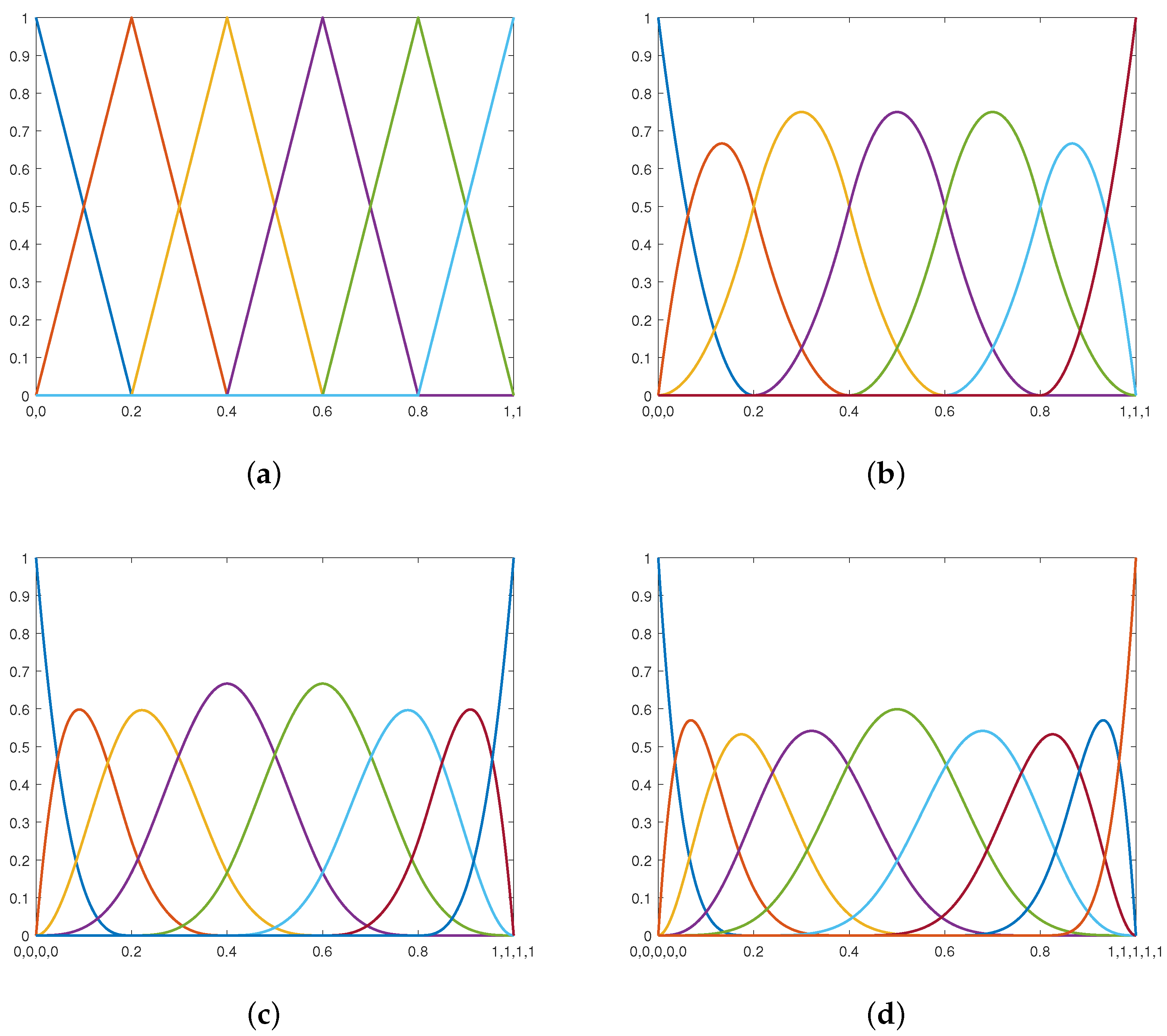
where $B_i^p\left(u\right)$ is the B-spline basis function and ${\omega }_i$ is the corresponding weight. In particular, when all the weights are 1, ${\left\{N_{i,p}\right\}}_{i=0,\cdots ,N}$ are equal to B-spline basis functions ${\left\{B_i^p\right\}}_{i=0,\cdots ,N}$. Figure 1 shows the B-spline basis functions under different orders with the same breakpoint sequence. Each parameter interval $[u_i,u_{i+1}]$ has $p+1$ related local bases, for which the property of local support is essential to the analysis.

For high-dimensional NURBS surfaces and solids, their blending basis functions are calculated by their tensor product [2].

$$\begin{array}{cc}\hfill N_{i,j;p,q}(u,v)& =\frac{B_i^p\left(u\right)B_j^q\left(v\right){\omega }_{i,j}}{{\sum }_{i^{\prime }=0}^n{\sum }_{j^{\prime }=0}^m{B}_{i^{\prime }}^p\left(u\right)B_{j^{\prime }}^q\left(v\right){\omega }_{i^{\prime },j^{\prime }}},\hfill \\ \hfill N_{i,j,k;p,q,r}(u,v,w)& =\frac{B_i^p\left(u\right)B_j^q\left(v\right)B_k^r\left(w\right){\omega }_{i,j,k}}{{\sum }_{i^{\prime }=0}^n{\sum }_{j^{\prime }=0}^m{\sum }_{k^{\prime }=0}^l{B}_i^p\left(u\right)B_{j^{\prime }}^q\left(v\right)B_{k^{\prime }}^r\left(w\right){\omega }_{i^{\prime },j^{\prime },k^{\prime }}}.\hfill \end{array}$$

(3)

Because of the tensor product structure of NURBS, local modification is inconvenient. The construction of NURBS representation is no picnic, since it always involves a good parameterization, smooth joining and trimming, etc. However, the NURBS representation of the geometry has the privilege of high order continuity, which possesses better smoothness. And the property that the geometry is always lied within the convex hull of the control mesh results in reduced degrees of freedom for computation. Local support makes it also cheap and easy to modify the geometry. In addition, NURBS can represent quadrics and free-form shapes.

2.2. IGA Galerkin Method

When Hughes et al. proposed IGA, the calculation was implemented by the Galerkin method [3] through the weak form of the differential equation. Here, we call it the IGA Galerkin method [1]. In analysis, NURBS geometry $\mathrm{\Omega }$ is regarded as the physical domain. Let the following Laplace equation over the physical domain be [5]

$$\begin{array}{cc}\hfill \Delta T+f& =0in\mathrm{\Omega },\hfill \\ \hfill T& =gon{\mathrm{\Gamma }}_D,\hfill \\ \hfill \nabla T·\mathbf{n}& =hon{\mathrm{\Gamma }}_N,\hfill \\ \hfill \beta T+\nabla T·\mathbf{n}& =ron{\mathrm{\Gamma }}_R,\hfill \end{array}$$

(4)

where the Dirichlet boundary ${\mathrm{\Gamma }}_D$, Neumann boundary ${\mathrm{\Gamma }}_N$, and Robin boundary ${\mathrm{\Gamma }}_R$ form the boundary $\partial \mathrm{\Omega }$. The functions f, g, h, and r are all given, and T is the unknown function to be solved. Without loss of generality, suppose that they are all scalar functions. We call Equation (4) the strong form of the partial differential Equation (PDE).

The IGA Galerkin method focuses on the weak form of PDE, which is obtained through Green’s theorem as follows:

$${\int }_{\mathrm{\Omega }}\nabla \omega ·\nabla Td\mathrm{\Omega }+\beta {\int }_{{\mathrm{\Gamma }}_R}\omega Td\mathrm{\Gamma }={\int }_{\mathrm{\Omega }}\omega f\mathrm{\Omega }+\beta {\int }_{{\mathrm{\Gamma }}_N}\omega hd\mathrm{\Gamma }+\beta {\int }_{{\mathrm{\Gamma }}_R}\omega rd\mathrm{\Gamma },$$

(5)

where the weighting function is $\omega \in \mathcal{V},\mathcal{V}=\left\{\omega \right|\omega \in H^1\left(\mathrm{\Omega }\right),\omega {|}_{{\mathrm{\Gamma }}_D}=0\}$, the trial solution is $T\in \mathcal{S},\mathcal{S}=\left\{T\right|T\in H^1\left(\mathrm{\Omega }\right),T{|}_{{\mathrm{\Gamma }}_D}=g\}$, and $H^1$ is a Sobolev space. The weak form (5) is then rewritten by a bilinear operator $a(·,·)$ and a linear form $L(·)$ as [5]

$$a(\omega ,T)=L\left(\omega \right).$$

(6)

Galerkin’s method constructs the finite-dimensional approximations of infinite spaces $\mathcal{S}$ and $\mathcal{V}$, i.e., ${\mathcal{S}}^h\in \mathcal{S},{\mathcal{V}}^h\in \mathcal{V}$. These approximate spaces are spanned by the same NURBS bases as the physical domain $\mathrm{\Omega }$. Let the unknown numerical solution $T_r$ be a linear combination of these basis functions with $N+1$ unknown coefficients, that is,

$$T_r\left(u\right)=\sum _{i=0}^N{N}_{i,p}\left(u\right)q_i.$$

(7)

Then, the weak form can be transformed into

$$a({\omega }_r,T_r)=L\left({\omega }_r\right).$$

(8)

By assembling the system of the weak form (8), we can solve the following linear equations and obtain the solution $T_r$ [5]:

$$\mathbf{Kq}=\mathbf{b}$$

(9)

where $\mathbf{q}$ refers to the unknown coefficients, $\mathbf{K}=\left[K_{i,j}\right]$ is the stiffness matrix, and $\mathbf{b}=\left[b_j\right]$ is the load vector given by

$$\begin{array}{cc}\hfill K_{i,j}& ={\int }_{\mathrm{\Omega }}\nabla N_i\nabla N_{j}d\mathrm{\Omega }+\beta {\int }_{{\mathrm{\Gamma }}_R}{N}_i{N}_{j}d\mathrm{\Gamma },\hfill \\ \hfill b_j& ={\int }_{\mathrm{\Omega }}{N}_{j}f\mathrm{\Omega }+\beta {\int }_{{\mathrm{\Gamma }}_N}{N}_{j}hd\mathrm{\Gamma }+\beta {\int }_{{\mathrm{\Gamma }}_R}{N}_{j}rd\mathrm{\Gamma }.\hfill \end{array}$$

(10)

For elastodynamic problems [3], the weak form often leads to solving the following Lagrangian dynamics Equation [5,7,8,9]:

$$\mathbf{M}\ddot{\mathbf{q}}\left(t\right)+\mathbf{C}\dot{\mathbf{q}}\left(t\right)+\mathbf{K}\mathbf{q}\left(t\right)=\mathbf{b}\left(t\right).$$

(11)

where $\mathbf{q}\left(t\right)$, $\dot{\mathbf{q}}\left(t\right)$, and $\ddot{\mathbf{q}}\left(t\right)$ are the displacement, velocity, and acceleration vectors, respectively. Stiffness matrix $\mathbf{K}=\left[{\mathbf{K}}_{i,j}\right]$ is related to partial derivative matrix $\mathbf{B}$ of the displacement and elastic coefficient matrix $\mathbf{D}$. $\mathbf{M}=\left[{\mathbf{M}}_{i,j}\right]$ is the mass matrix given by mass density $\rho$. $\mathbf{C}$ is the damping matrix, which can be represented by the mass and stiffness matrices according to Rayleigh damping coefficients ${\gamma }_1$ and ${\gamma }_2$. $\mathbf{b}\left(t\right)=\left[{\mathbf{b}}_i\left(t\right)\right]$ is the force vector given by external force $\mathbf{f}\left(t\right)$.

$$\begin{array}{cc}\hfill {\mathbf{M}}_{i,j}& ={\int }_{\mathrm{\Omega }}{N}_i\rho N_{j}d\mathrm{\Omega }\mathbf{I},\hfill \\ \hfill {\mathbf{K}}_{i,j}& ={\int }_{\mathrm{\Omega }}{\left(\mathbf{B}{N}_i\right)}^T\mathbf{D}\left(\mathbf{B}{N}_j\right)d\mathrm{\Omega },\hfill \\ \hfill {\mathbf{b}}_j\left(t\right)& ={\int }_{\mathrm{\Omega }}{N}_j{\mathbf{f}}_j\left(t\right)d\mathrm{\Omega },\hfill \\ \hfill \mathbf{C}& ={\gamma }_1\mathbf{M}+{\gamma }_2\mathbf{K}.\hfill \end{array}$$

(12)

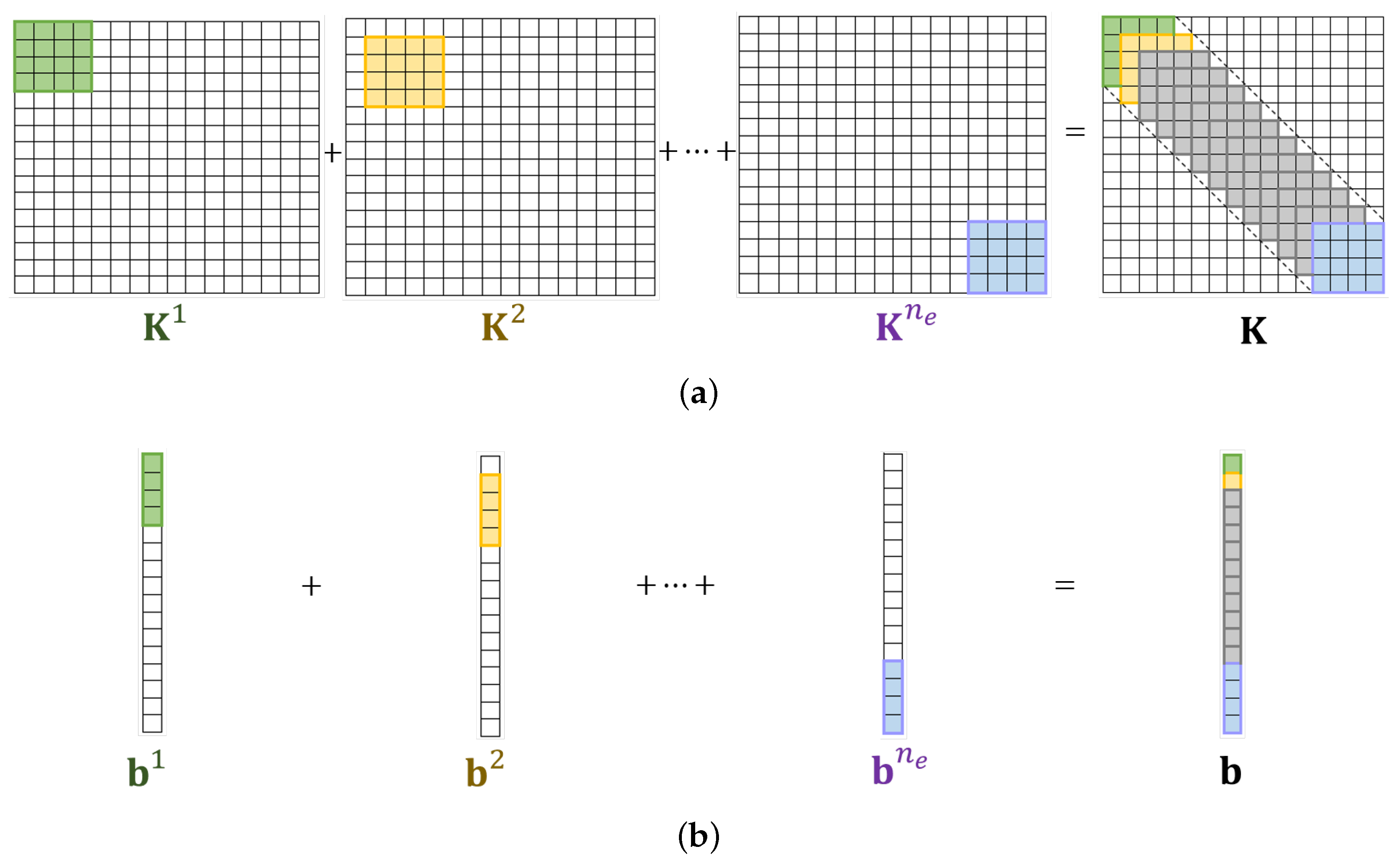
Given the local support of the NURBS basis, the assembly can be treated as the sum of the counterparts of elements according to their contribution. Thus, the calculation in the whole physical domain is transferred to the calculation on each element (Figure 2), which reduces the computational cost. The assembly involves integration on the physical domain, so some numerical integration technologies on the reference space arise to improve the calculation. Another issue is that the condition number of the assembled stiffness matrix can be large, especially in the presence of large DoFs. This issue can be alleviated by pre-conditioning operations [10,11,12,13] and high-quality parameterization schemes [14,15,16,17,18,19,20,21,22,23,24].

2.3. Isogeometric Collocation Method

When the degree of the NURBS basis used in IGA is higher than the order of the differential equation, the form of the equation still exists if the NURBS-expressed numerical solution is introduced into the differential equation. Then, we can select a number of points in the computational domain, introduce these points into the equation form above, and obtain a linear system. The unknowns in the equations are the unknown coefficients of NURBS functions. This is the isogeometric collocation (IGA-C) method [6] proposed by Auricchio et al. in 2010, where the points selected in the calculation domain are called collocation points. The convergence and consistency of some theoretical results of IGA-C have been examined and proven by Lin et al. [25,26]. Distinguished from IGA Galerkin, which focuses on the weak form, IGA-C directly deals with the strong form of PDE. More generally, the boundary value problem (BVP) can be summarized as follows [6]:

$$\left\{\begin{array}{cc}\mathfrak{L}T=f\hfill & in\mathrm{\Omega },\hfill \\ \mathfrak{G}T=g\hfill & on\partial \mathrm{\Omega },\hfill \end{array}\right.$$

(13)

where $\mathfrak{L}$ represents a scalar differential operator, T is the unknown solution, and the given right-hand side f is called the load function. The boundary vector operator $\mathfrak{G}T$ represents the boundary conditions.

IGA-C solves the equations by introducing a set of collocation points ${\left\{{\overline{\mathbf{u}}}_k\right\}}_{k=0,\dots ,N_{int}}$ into parametric domain $\widehat{\mathrm{\Omega }}$ and ${\left\{{\overline{\mathbf{u}}}_k\right\}}_{k=N_{int}+1,\dots ,N_{int}+N_{bd}}$ on the boundary of parametric domain $\partial \widehat{\mathrm{\Omega }}$. The corresponding points of the physical domain are ${\overline{\mathbf{x}}}_k=\mathbf{F}\left({\overline{\mathbf{u}}}_k\right),k=0,\dots ,N_{int}+N_{bd}$, where $\mathbf{F}$ is the NURBS mapping defined in Section 2.1. Thus, replacing the unknown T of BVP with the expression of $T_r$ at ${\left\{{\overline{\mathbf{x}}}_k\right\}}_{i=0,\dots ,N_{int}+N_{bd}}$ leads to a linear system.

$$\left\{\begin{array}{cc}\mathfrak{L}{T}_r\left({\overline{\mathbf{x}}}_k\right)=f\left({\overline{\mathbf{x}}}_k\right)\hfill & k=0,\dots ,N_{int},\hfill \\ \mathfrak{G}{T}_r\left({\overline{\mathbf{x}}}_k\right)=g\left({\overline{\mathbf{x}}}_k\right)\hfill & k=N_{int}+1,\dots ,N_{int}+N_{bd}.\hfill \end{array}\right.$$

(14)

The coefficient matrix of the linear system is called the collocation matrix. In the system obtained from the IGA-C framework, the number of equations is equal to the number of unknowns, i.e., $N_{int}+N_{bd}=N$. Direct solving and solving with iterative methods can be adopted to solve the linear system. Given that the partial differential operator acts on the physical coordinates, and the NURBS solution is a function of the parametric coordinates, the derivatives can be implemented by the chain rule. For instance, the derivatives of the 3D case involve the following calculations:

$$\frac{\partial T_r}{\partial x_i}=\frac{\partial T_r}{\partial u}\frac{\partial u}{\partial x_i}+\frac{\partial T_r}{\partial v}\frac{\partial v}{\partial x_i}+\frac{\partial T_r}{\partial w}\frac{\partial w}{\partial x_i},$$

(15)

$$\begin{array}{cc}\hfill \frac{{\partial }^2{T}_r}{\partial x_i\partial x_j}& =\left(\frac{\partial u}{\partial x_i}\frac{\partial u}{\partial x_j}\right)\frac{{\partial }^2{T}_r}{\partial u^2}+(\frac{\partial u}{\partial x_i}\frac{\partial v}{\partial x_j}+\frac{\partial v}{\partial x_i}\frac{\partial u}{\partial x_j})\frac{{\partial }^2{T}_r}{\partial u\partial v}+(\frac{\partial u}{\partial x_i}\frac{\partial w}{\partial x_j}+\frac{\partial w}{\partial x_i}\frac{\partial u}{\partial x_j})\frac{{\partial }^2{T}_r}{\partial u\partial w}+\hfill \\ \hfill & \left(\frac{\partial v}{\partial x_i}\frac{\partial v}{\partial x_j}\right)\frac{{\partial }^2{T}_r}{\partial v^2}+(\frac{\partial v}{\partial x_i}\frac{\partial w}{\partial x_j}+\frac{\partial w}{\partial x_i}\frac{\partial v}{\partial x_j})\frac{{\partial }^2{T}_r}{\partial vs.\partial w}+\left(\frac{\partial w}{\partial x_i}\frac{\partial w}{\partial x_j}\right)\frac{{\partial }^2{T}_r}{\partial w^2}+\hfill \\ \hfill & (\frac{{\partial }^{2}u}{\partial x_i\partial x_j}\frac{\partial T_r}{\partial u}+\frac{{\partial }^{2}v}{\partial x_i\partial x_j}\frac{\partial T_r}{\partial v}+\frac{{\partial }^{2}w}{\partial x_i\partial x_j}\frac{\partial T_r}{\partial w}),\hfill \end{array}$$

(16)

where $x_i,x_j$ refer to any one component of the physical coordinate $\mathbf{x}={[x,y,z]}^T$ calculated by the NURBS mapping $\mathbf{x}={\sum }_{i=0}^{n\times m\times l}{N}_{i,j,k}\left(\overline{\mathbf{u}}\right){\mathbf{P}}_{i,j,k}$, where $\overline{\mathbf{u}}$ is the collocation point. The parametric coordinate is $\mathbf{u}={[u,v,w]}^T$, and the partial derivatives can be calculated as follows:

$$\begin{array}{cc}\hfill \frac{\partial \mathbf{u}}{\partial \mathbf{x}}& =\left[\begin{array}{ccc}\frac{\partial u}{\partial x}& \frac{\partial u}{\partial y}& \frac{\partial u}{\partial z}\\ \frac{\partial v}{\partial x}& \frac{\partial v}{\partial y}& \frac{\partial v}{\partial z}\\ \frac{\partial w}{\partial x}& \frac{\partial w}{\partial y}& \frac{\partial w}{\partial z}\end{array}\right]={\left[\begin{array}{ccc}\frac{\partial x}{\partial u}& \frac{\partial x}{\partial v}& \frac{\partial x}{\partial w}\\ \frac{\partial y}{\partial u}& \frac{\partial y}{\partial v}& \frac{\partial y}{\partial w}\\ \frac{\partial z}{\partial u}& \frac{\partial z}{\partial v}& \frac{\partial z}{\partial w}\end{array}\right]}^{-1}={\left(\frac{\partial \mathbf{x}}{\partial \mathbf{u}}\right)}^{-1},\hfill \\ \hfill {\left(\frac{{\partial }^2\mathbf{u}}{\partial {\mathbf{x}}^2}\right)}^T& =\left[\begin{array}{ccc}\frac{{\partial }^{2}u}{\partial x^2}& \frac{{\partial }^{2}v}{\partial x^2}& \frac{{\partial }^{2}w}{\partial x^2}\\ \frac{{\partial }^{2}u}{\partial y^2}& \frac{{\partial }^{2}v}{\partial y^2}& \frac{{\partial }^{2}w}{\partial y^2}\\ \frac{{\partial }^{2}u}{\partial z^2}& \frac{{\partial }^{2}v}{\partial z^2}& \frac{{\partial }^{2}w}{\partial z^2}\end{array}\right]=-{\left({\mathbf{D}}_1{\mathbf{D}}_2\right)}^{-1}\frac{\partial \mathbf{u}}{\partial \mathbf{x}},\hfill \end{array}$$

(17)

where

$$\begin{array}{cc}\hfill {\mathbf{D}}_1& =\left[\begin{array}{cccccc}{\left(\frac{\partial u}{\partial x}\right)}^2& 2\frac{\partial u}{\partial x}\frac{\partial v}{\partial x}& 2\frac{\partial u}{\partial x}\frac{\partial w}{\partial x}& {\left(\frac{\partial v}{\partial x}\right)}^2& 2\frac{\partial v}{\partial x}\frac{\partial w}{\partial x}& {\left(\frac{\partial w}{\partial x}\right)}^2\\ {\left(\frac{\partial u}{\partial y}\right)}^2& 2\frac{\partial u}{\partial y}\frac{\partial v}{\partial y}& 2\frac{\partial u}{\partial y}\frac{\partial w}{\partial y}& {\left(\frac{\partial v}{\partial y}\right)}^2& 2\frac{\partial v}{\partial y}\frac{\partial w}{\partial y}& {\left(\frac{\partial w}{\partial y}\right)}^2\\ {\left(\frac{\partial u}{\partial z}\right)}^2& 2\frac{\partial u}{\partial z}\frac{\partial v}{\partial z}& 2\frac{\partial u}{\partial z}\frac{\partial w}{\partial z}& {\left(\frac{\partial v}{\partial z}\right)}^2& 2\frac{\partial v}{\partial z}\frac{\partial w}{\partial z}& {\left(\frac{\partial w}{\partial z}\right)}^2\end{array}\right]\hfill \\ \hfill {\mathbf{D}}_2& =\left[\begin{array}{ccc}\frac{{\partial }^{2}x}{\partial u^2}& \frac{{\partial }^{2}y}{\partial u^2}& \frac{{\partial }^{2}z}{\partial u^2}\\ \frac{{\partial }^{2}x}{\partial u\partial v}& \frac{{\partial }^{2}y}{\partial u\partial v}& \frac{{\partial }^{2}z}{\partial u\partial v}\\ \frac{{\partial }^{2}x}{\partial u\partial w}& \frac{{\partial }^{2}y}{\partial u\partial w}& \frac{{\partial }^{2}z}{\partial u\partial w}\\ \frac{{\partial }^{2}x}{\partial v^2}& \frac{{\partial }^{2}y}{\partial v^2}& \frac{{\partial }^{2}z}{\partial v^2}\\ \frac{{\partial }^{2}x}{\partial vs.\partial w}& \frac{{\partial }^{2}y}{\partial vs.\partial w}& \frac{{\partial }^{2}z}{\partial vs.\partial w}\\ \frac{{\partial }^{2}x}{\partial w^2}& \frac{{\partial }^{2}y}{\partial w^2}& \frac{{\partial }^{2}z}{\partial w^2}\end{array}\right].\hfill \end{array}$$

When the number of selected collocation points is larger than the number of unknown coefficients, i.e., $N_{int}+N_{bd}>N$, which indicates that the collocation matrix in the system is over-determined, the linear system can be solved in a least-squares manner [6,27,28]. On the basis of this idea, Lin et al. [27] proposed the isogeometric least-squares collocation method (IGA-L) and presented the conditions and theoretical proof for convergence and consistency. The numerical results of the IGA-L method validate the increased accuracy obtained by adopting numerous collocation points.

It is worth mentioning that the original application of IGA-C was on the physical domain constructed by NURBS in simulation, and later there were advanced IGA-C corresponding to more splines. Due to the exploit of NURBS, the privileges of IGA-C can be concluded as a high-order continuity of the solution and high efficiency for computation. Nevertheless, if the collocation points are not properly selected, the condition number of the coefficient matrix of the generated linear system may be very large, or even singular. Thus, the collocation schemes become crucial to the effectiveness and accuracy of IGA-C.

2.4. Comparison of IGA Galerkin and IGA-C

IGA Galerkin has stable calculation, a high convergence rate, and perfect theoretical analysis [1]. However, it requires a large amount of integration calculation, and the assembly of the stiffness matrix is highly complex. The integration efficiency of IGA was first considered by Reference [29]. Then, Gauss–Galerkin quadrature rules [30] and optimal and reduced quadrature rules [31] were developed. A promising approach for reusing the basis function evaluations in numerical integration has been recently presented to improve the accuracy and time cost [32].

The commonly used tensor product NURBS basis must be reparameterized globally when performing refinements, which adds a number of unnecessary DoFs to the system. To reduce the computational burden, Bazilevs et al. [33] explored T-splines with IGA for local refinement and provided the alternatives of the adoption of the bases. Several alternative spline technologies have been proposed as a basis for IGA. In addition to T-splines [34], hierarchical B-splines (HB-splines) [35,36,37,38], truncated hierarchical B-splines (THB-splines) [39], polynomial splines over hierarchical T-meshes (PHT-splines) [40,41,42], locally refined splines (LR-splines) [43], and hierarchical extension of analysis-suitable T-splines (HASTS) [44] are also capable of adaptive local refinement in IGA. By adopting non-polynomial functions, such as trigonometric or hyperbolic functions, generalized B-splines [45,46] and generalized T-splines [47] enhance the piecewise polynomial spline bases for analysis. For discontinuous problems, such as cracks, the extended finite element method (XFEM) [48] incorporates a discontinuous displacement field and asymptotic crack tip displacement fields into the displacement approximation through the partition of unity method. Developed from the concept of XFEM, IGA has been enhanced to extended IGA (XIGA) [49,50] to locally enrich the bases for simulating discontinuities and singular fields. In accordance with the crack location, the original bases in the area can be selected to split into several new bases multiplied by an enrichment function and then contribute to the overall approximation. In addition to crack problems, enrichment functions can be custom designed for other specific problems, such as imitating local refinement when using the splitting basis techniques in XIGA [51]. An overview of the computer implementation aspects of IGA can be found in Reference [52].

In particular, IGA Galerkin requires high-quality parameterization of the computational domain. If singular points exist, the system may suffer from collapse unless a special treatment is provided. Cohen et al. [53] proposed the concept of analysis-aware modelling to show that the quality of domain parameterization has a great impact on the analysis results and efficiency [54], and that the condition number of the assembled stiffness matrix affects the stability of the linear system to be solved [55]. The research on analysis-suitable planar [14,15,16,17,18,19] and volumetric [20,21,22,23,24] parameterization for IGA has gradually flourished. Moreover, Xu et al. attempted to decouple geometry and simulation and obtained satisfactory results [56]. They revealed that the bases for the solution space are not necessarily the same with the bases for the physical domain. Overall, constructing high-quality analysis-suitable parameterization from a complex CAD boundary is still an open problem. In conclusion, the interests of IGA Galerkin are focused on the following aspects:

• Numerical quadrature rules in the assembly;
• High-quality parameterization for IGA-suitable analysis;
• Construction of alternative basis functions for particular cases.

IGA-C was proposed for accelerating the solving of PDEs by avoiding the efficiency issue of numerical integration in IGA Galerkin. It focuses on solving the strong form of PDEs rather than the weak form in IGA Galerkin to increase the accuracy-to-computational cost ratio [6,36]. IGA-C considers the superior accuracy and smoothness of NURBS basis functions and the low computational cost, which is a compromise between accuracy and computational time. The assembly of the stiffness matrix becomes simple and easy, and the bandwidth of the matrix becomes narrow. Substituting the derivatives of the NURBS numerical solution at some collocation points into PDE leads directly to a linear system. The number of equations (i.e., the collocation points) in the system can be equal to or greater than the number of unknown coefficients of NURBS functions. The solution (or the least-squares solution) of the system determines the coefficients of the NURBS function as the numerical solution of PDE.

Compared with the IGA Galerkin method, the IGA-C method has many merits. First, the calculation amount is small, and the calculation speed is fast. Second, the form is simple and flexible, and the linear equations of the IGA-C are easy to construct. Lastly, even in the presence of singular points, IGA-C calculation can still be carried out as long as appropriate collocation points are selected.

To date, the most popular numerical methods in solving PDEs are finite difference method (FDM) and finite element method (FEM). FDM uses the difference to replace the exact derivative, which is fast but loses some precision in derivative approximation. FEM solves the variational form (weak form) equivalent to the original problem (strong form), in which the quadrature in the generated linear system is treated numerically. Both methods require mesh generation of the computational domain. The biggest difference between IGA-C methods and classical FDM and FEM is that IGA-C methods avoid mesh generation, because the computational field and the physical field are the same and are both represented by NURBS. Moreover, the degrees of freedom of IGA-C refer to the number of control points, which is much less than the degrees of freedom in FDM and FEM, which refer to the number of mesh nodes. Because IGA Galerkin also needs complex quadrature computation in weak form similar to FEM, whereas IGA-C methods select some appropriate collocation points by collocation scheme and substitute them into the strong form directly for solving, IGA-C is much easier and faster to implement than other numerical methods. With the high accuracy-to-computational-time ratio, the research on IGA-C methods and their applications is significant.

However, the theoretical system of the IGA-C method is far from being established. Lin et al. revealed the conditions for the consistency and convergence of IGA-C and IGA-L methods with the stable or strongly monotonic differential operator and provided the proof in their work [25,27]. In existing work, the convergence rate was mostly verified by numerical examples. Lin et al. also deduced the convergence rate and developed the necessary and sufficient conditions for the consistency of the IGA-C method [26]. The IGA-C method is consistent if and only if the differential operator in BVP and the interpolation operator on the load function are uniformly bounded when the knot grid size tends to zero, which advances the numerical analysis of the IGA-C method.

Moreover, the calculation accuracy and convergence rate of IGA-C are not high. These defects seriously restrict the further application and development of the IGA-C method. A few studies have focused on how to select ideal collocation points for the parameterization of a given domain to improve the convergence rate of IGA-C [28,57,58,59,60]. In fact, many factors, such as the parameterization quality of the computational domain [61,62], the collocation selection scheme [28,57,58,59,60], and the differential equation [63,64], affect the convergence rate and calculation accuracy. The current work does not consider the comprehensive impact of multiple factors on the IGA-C method. Therefore, the urgent tasks for current studies on IGA-C can be summarized as follows:

• Clarification of the consistency and convergence conditions;
• Design of efficient collocation schemes;
• Improvement of calculation accuracy and speed.

2.5. IGA-CL and IGA-GL Methods

When solving an IGA problem, the exact solution is usually unknown, and the approximation error is difficult to estimate. The problem lies in the determination of how many degrees of freedom are needed to realize acceptable accuracy and when to stop the refinement. Motivated by this problem, the PDE $\mathfrak{L}T=f$ with the strongly stable differential operator $\mathfrak{L}$ can be solved with IGA methods by fitting the load function f [25,27,65]. The exploitation of the load function can control the error estimation. The approximation error of numerical solution $T_r$ no longer requires the exact solution $T^{*}$ of PDE as a prior. Without knowing $T^{*}$ when calculating the error $\parallel T^{*}-T_r{\parallel }_2$, the approximation error takes good advantage of load function f, which is defined as

$$e_r={\parallel f-\mathfrak{L}{T}_r\parallel }_2.$$

(18)

According to the necessary and sufficient condition for the consistency of the IGA-C method [26], suppose $\mathfrak{L}$ is the differential operator in BVP (13), ${\mathcal{I}}^{\rho }$ is an interpolation operator satisfying ${\mathcal{I}}^{\rho }f=\mathfrak{L}{T}_r$, $T_r$ is the IGA-C numerical solution, the IGA-C method is consistent if and only if $\mathfrak{L}$ and ${\mathcal{I}}^{\rho }$ are both uniformly bounded when knot grid size $\rho \to 0$, i.e.,

$$\parallel \mathfrak{L}{T}^{*}-\mathfrak{L}{T}_r{\parallel }_2\to 0,when\rho \to 0.$$

(19)

Because IGA-CL is actually a knot insertion of the initial parameter space for constructing numerical solutions in IGA-C, the essence of IGA-CL solution is the IGA-C solution. Then, with $\mathfrak{L}{T}^{*}=f$ holding, we can obtain

$$\parallel f-\mathfrak{L}{T}_r{\parallel }_2\to 0,when\rho \to 0.$$

(20)

Thus, the necessary and sufficient condition for the consistency of the IGA-CL method is derived as well.

Specifically, in a typical IGA, the knot vector of the NURBS numerical solution is determined only by the physical domain. On the one hand, solving PDE with IGA is regarded as fitting load function f defined on the NURBS geometry $\mathrm{\Omega }$ with the differential operator on the NURBS numerical solution $\mathfrak{L}{T}_r$. On the other hand, in the area of data fitting in geometric design, the design of the knot vector has a close relationship with the NURBS functions to be fitted. Therefore, the detected feature points of the load function are integrated into the initial knot vector of the physical domain to construct the new knot vector of the numerical solution in the IGA framework. The concept of combining the information from the load function and physical domain to improve accuracy applies not only to the IGA-C framework but also to the IGA Galerkin framework, which are referred to as IGA-CL and IGA-GL methods, respectively.

Thus, given a PDE defined on the NURBS physical domain, we can always apply the feature detection strategy to the load function and generate the improved knot vector for the NURBS solution with high accuracy using IGA-GL and IGA-CL methods. The error estimation becomes easy to control without the exact solution.

3. Collocation Schemes and Convergence

The selection of collocation points influences the efficiency of IGA-C greatly, and it is the crucial part of the procedure because it directly affects the accuracy and convergence of the numerical solution. Some popular options, such as Demko and Greville abscissae [6,57], superconvergent (SC) points [28], Cauchy–Galerkin (CG) points [58], and alternating/clustered superconvergent (ASC/CSC) points [59], have been widely utilized in IGA-C problems since they were proposed. In this section, we introduce commonly used collocation schemes.

3.1. Demko and Greville Abscissae

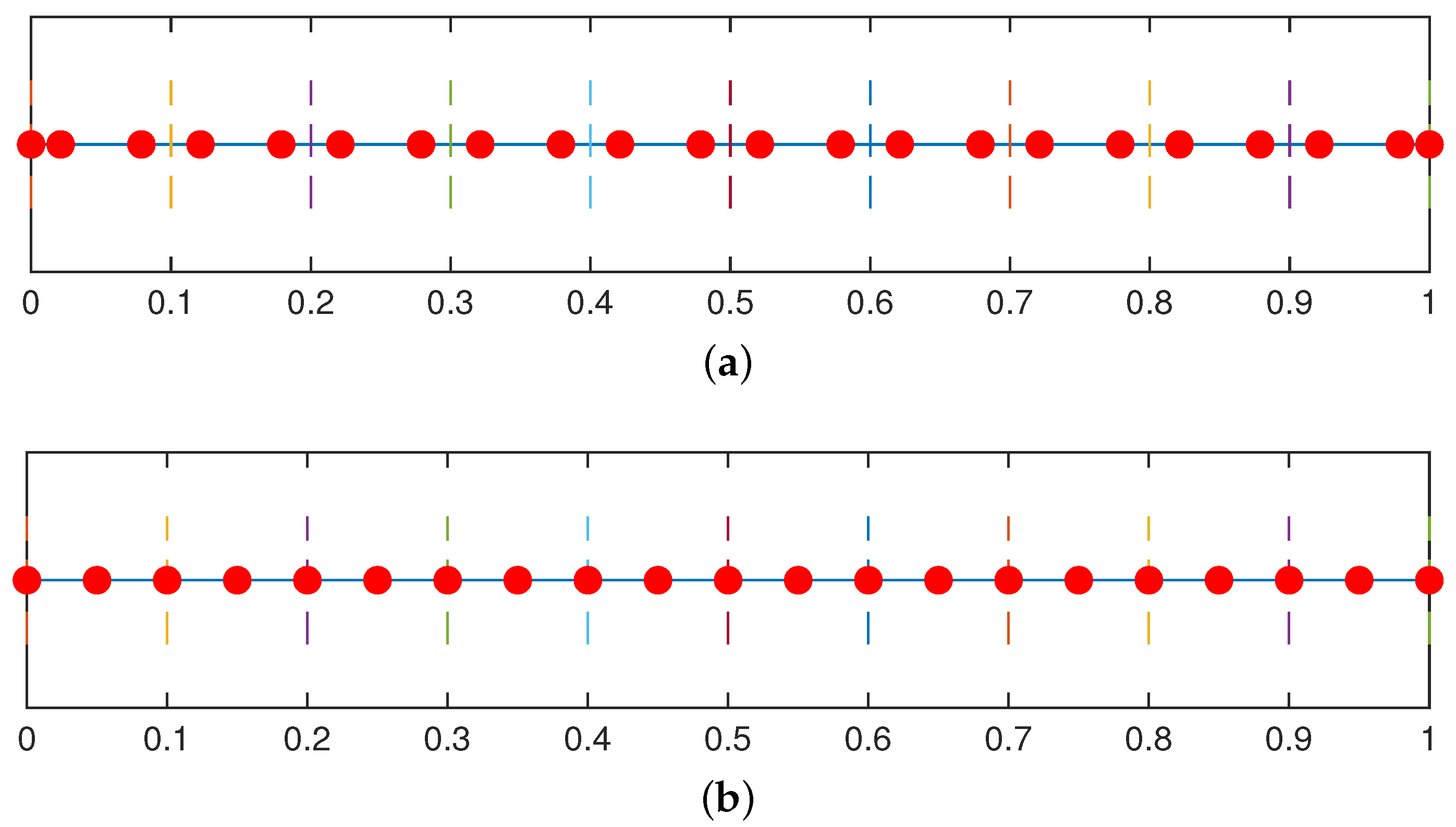
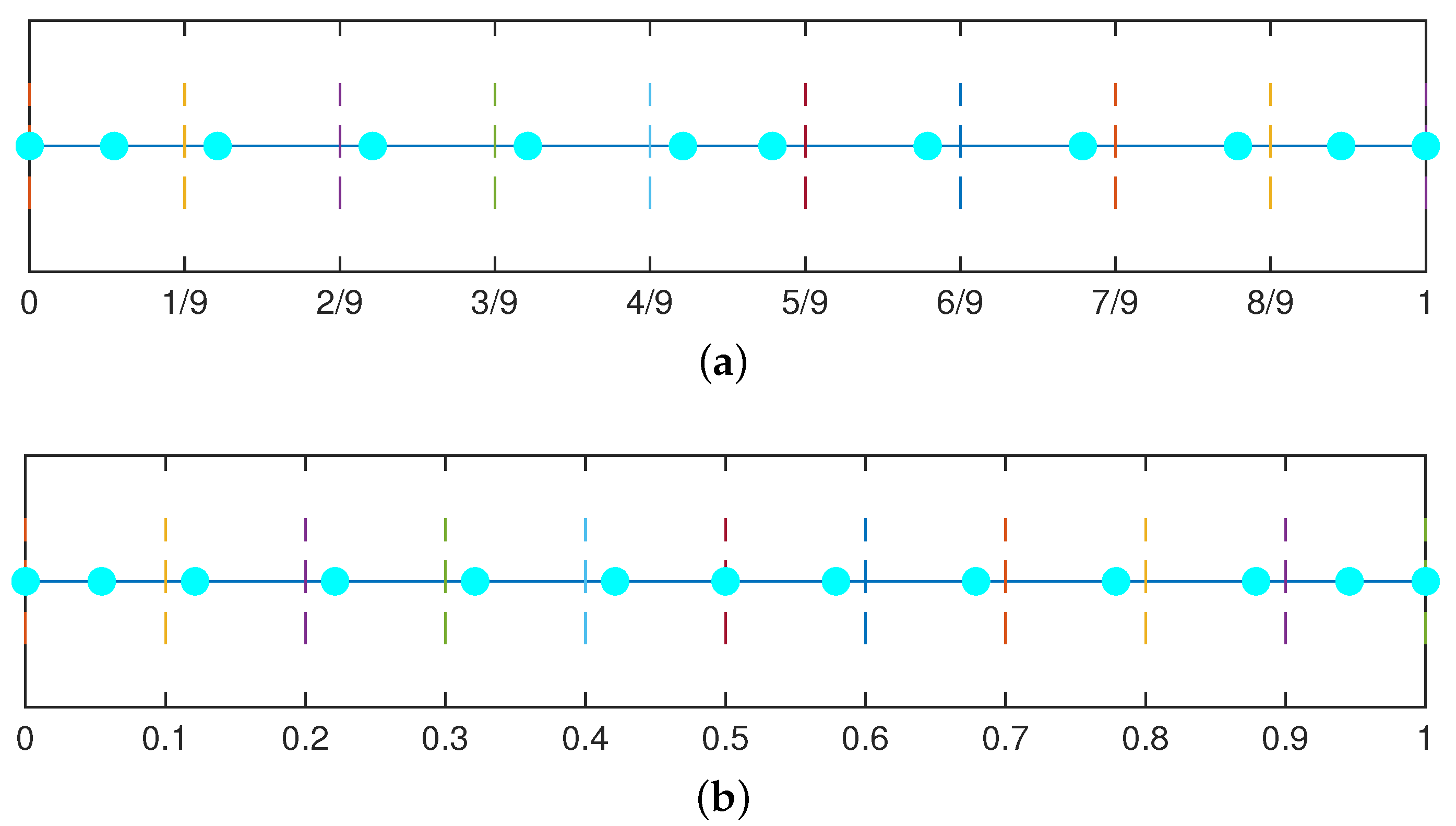
In IGA-C, the commonly used collocation points are Demko [57] and Greville [6] abscissae. Demko abscissae are obtained from the extreme points of Chebyshev splines and can be calculated by the function “chbpnt” in MATLAB or by referring to the book by deBoor [66]. They are proven to be stable for any mesh and degree. Greville abscissae are acquired from the averaging operation of the knot vector. However, the convergence orders of both choices are $\mathcal{O}\left(h^{p-1}\right)$ for the odd degree p of the NURBS bases and $\mathcal{O}\left(h^p\right)$ for the even degree p.

Assuming that the NURBS basis for the numerical solution is associated with an open knot vector $U=\{u_0,u_1,\dots ,u_{N+p+1}\}$ with multiplicity $p+1$ at both ends, Greville collocation points are generated via an averaging operation as follows [6]:

$${\tau }_j=\frac{1}{p}\sum _{i=j}^{j+p-1}{u}_i,j=1,2,...,N+1.$$

(21)

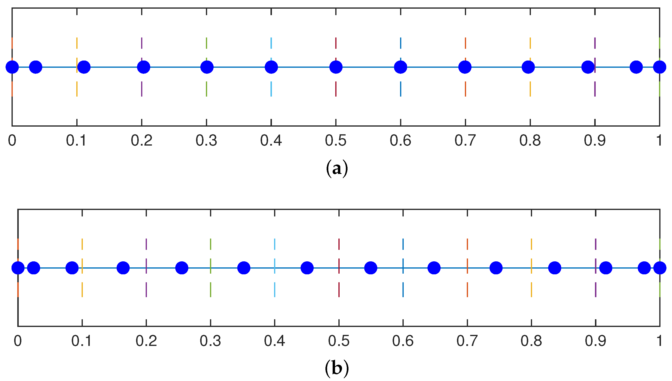
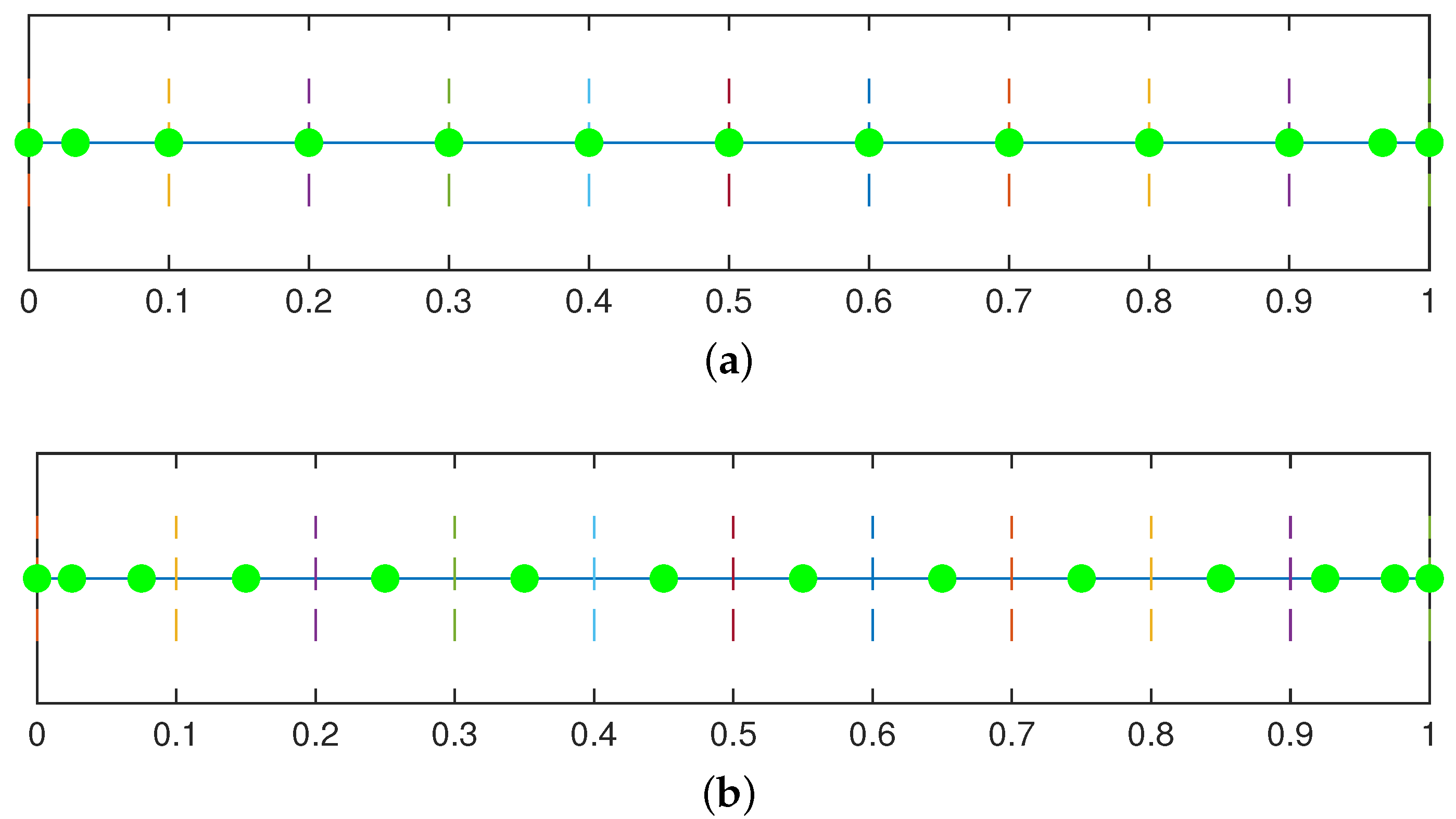
Figure 3 and Figure 4 display the distribution of Demko and Greville points under odd and even degrees. Each knot interval includes at least one collocation point, and the number of generated collocation points is equal to the number of unknown coefficients $N+1$. Except for points near the boundary, Greville points locate exactly on the knot positions for an odd degree, and Greville points locate exactly on the centre of the knot intervals for an even degree. Demko points are very close to Greville points but not quite equal.

3.2. Superconvergent Points

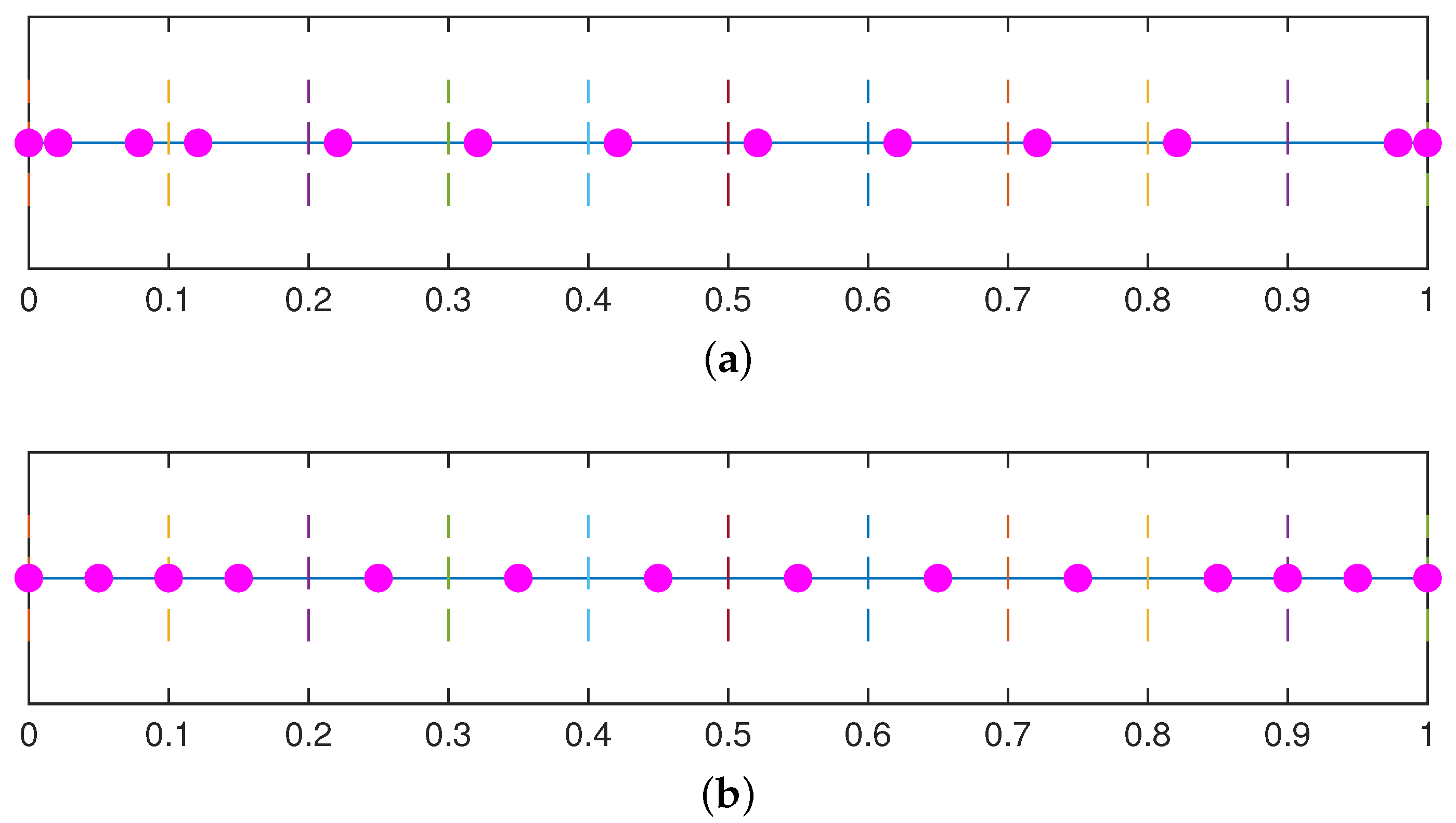
On the basis of superconvergent theory, Anitescu et al. developed superconvergent points (SC points) [28] to increase the convergence rate.

They attempted to find collocation points in which the collocation solution behaves similarly to the standard Galerkin solution. On the basis of the observation that the error in the second derivative for collocation approximation is the smallest at the collocation points, they sought for the collocation points in which the error in the second derivatives of Galerkin approximation is also small. The computed numerical solution is expected to be close to the Galerkin numerical solution up to higher-order terms as well. The problems are that the accuracy of SC points are not high enough and that there are nearly twice as many points as DoFs. Given that the SC points are all adopted as collocation points, a solution of the overdetermined linear system needs to be computed by least-squares approximation. Anitescu et al. improved the convergence order of the IGA-C solution to the optimal $\mathcal{O}\left(h^{p+1}\right)$ for odd degree p and kept one-order suboptimal $\mathcal{O}(h^p$) for the even degree.

Table 1. Superconvergent points in the reference interval $[-1,1]$ [28].

Degree	Second Derivative Superconvergent Points
$p=3$	$-\frac{1}{\sqrt{3}},\frac{1}{\sqrt{3}}$
$p=4$	$-1,0,1$
$p=5$	$-\frac{\sqrt{225-30\sqrt{3}}}{15},\frac{\sqrt{225-30\sqrt{3}}}{15}$
$p=6$	$-1,0,1$
$p=7$	$-0.50491856751,0.50491856751$

SC points are equal to Greville points when p = 2.

[28] lists the locations of superconvergent points in the reference domain $[-1,1]$ under different degrees. The SC points are generated from the reference domain $[-1,1]$ to the knot interval $[u_i,u_{i+1}],i=p,\dots ,N-p-1$ in proportion to the superconvergence point. We present the distributions of SC points under odd and even degrees (e.g., $p=3$ and $p=4$) in Figure 5. Except for points near the boundary, at least two symmetric SC collocation points exist in each knot interval for the odd degree, whereas SC points are located at the centre and both ends for the even degree. The numbers of SC points are $2(N+1-p)+2$ and $2(N+1-p)+1$ for odd and even cases, respectively, which are greater than the number of unknown coefficients $N+1$ and are solved in a least-squares manner.

3.3. Cauchy–Galerkin Points

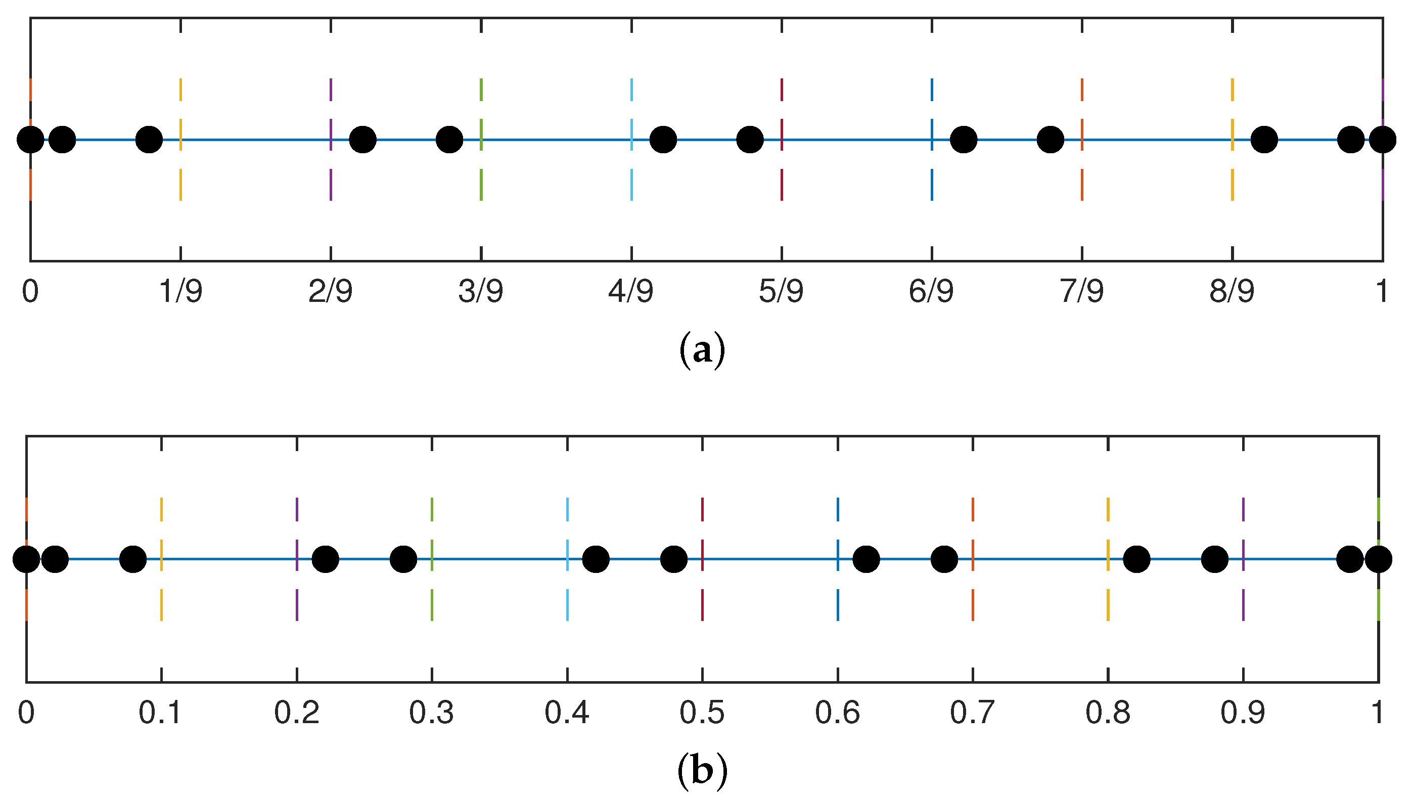
Cauchy–Galerkin points (CG points) have been proven to exist such that the IGA-C solution at these points can coincide with the IGA Galerkin solution [58]. CG points are selected as a certain subset of the zeros of the Galerkin residual, i.e., SC points (Table 1). Under some hypotheses, these approximated CG points achieve superconvergence of the second derivatives of the Galerkin solution. IGA-C with CG points has been verified to have the convergence order of $\mathcal{O}\left(h^p\right)$ for both odd and even degrees.

Figure 6 depicts the distribution of CG points, which preserves one SC point in each knot interval while maintaining the global symmetry as well. Thus, the number of CG points is equal to DoFs $N+1$.

3.4. Alternating/Clustered Superconvergent Points

Montardini et al. found a subset of SC points and obtained the optimal convergence order $\mathcal{O}\left(h^{p+1}\right)$ for odd degree p [59]. They were inspired by the selection way of CG points and devised a scheme of alternating SC point selection (ASC), which chooses collocation points from every other SC point. The collocation points in the elements near the boundary can be chosen flexibly without affecting the convergence rate. Examples of the distribution of ASC points are shown in Figure 7.

Furthermore, Montardini et al. attempted to acquire a globally periodic distribution of collocation points while maintaining the symmetry at the local element scale. The collocation points are selected as two SC points for every other element, which is shown in a clustered way. We call these clustered SC points (CSC points).

Figure 8 illustrates an instance of the clustered scheme under odd and even numbers of elements for the odd degree. The collocation points near the boundary are determined by considering the DoFs, symmetry, and periodicity.

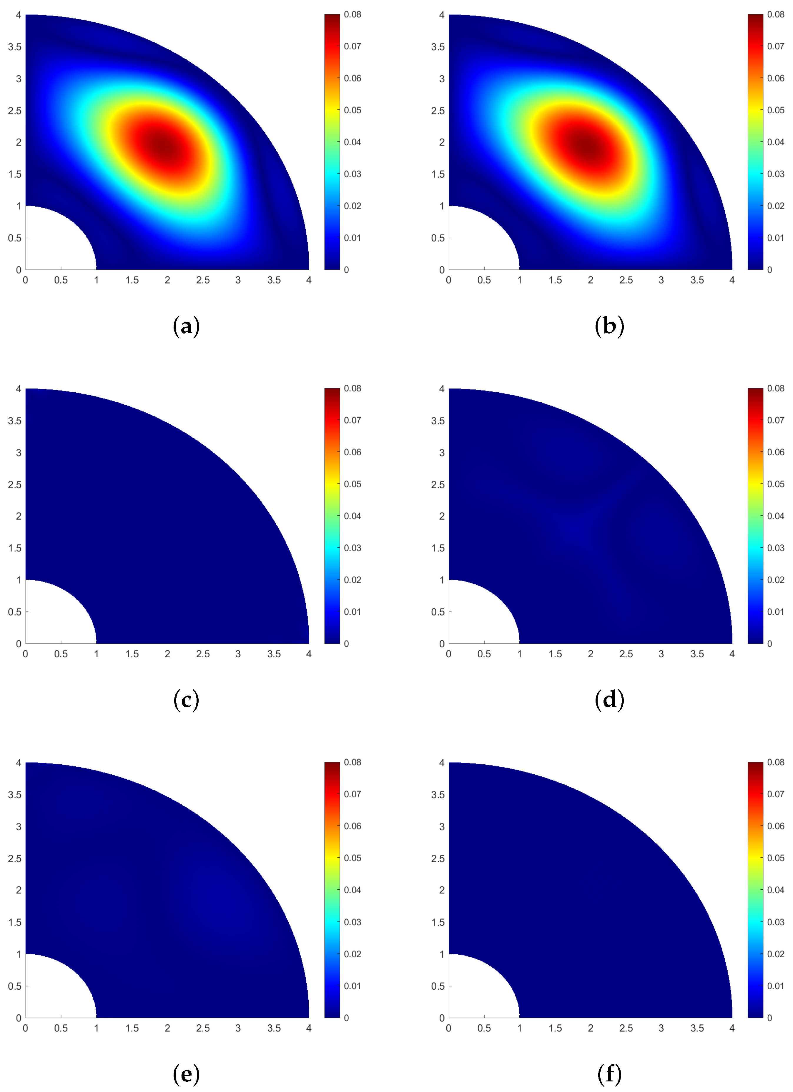
To compare these collocation schemes, we present an example of numerical experimental results under different collocation schemes in Figure 9. Here, we solve the source problem in reference [26] defined on a quarter of an annulus with degree $p=3$, and we display the absolute errors of the IGA-C numerical solutions with different collocation schemes after some $h-$refinements. Specifically, the relative errors in $L_2$ norm are shown in

Table 2. Relative errors in $L_2$ norm of IGA-C with different collocation schemes after twice $h-$refinements ($p=3$).

IGA-C Methods	169 DoFs	529 DoFs	1849 DoFs
Greville	$2.321\times {10}^{-2}$	$5.578\times {10}^{-3}$	$1.380\times {10}^{-3}$
Demko	$2.481\times {10}^{-2}$	$5.817\times {10}^{-3}$	$1.398\times {10}^{-3}$
SC	$2.482\times {10}^{-3}$	$1.059\times {10}^{-4}$	$6.992\times {10}^{-6}$
CG	$2.725\times {10}^{-3}$	$2.903\times {10}^{-4}$	$3.495\times {10}^{-5}$
ASC	$2.658\times {10}^{-3}$	$3.183\times {10}^{-4}$	$3.944\times {10}^{-5}$
CSC	$1.481\times {10}^{-3}$	$7.941\times {10}^{-5}$	$4.934\times {10}^{-6}$

. Finally, we compare the convergence rates of the above-mentioned collocation schemes under odd and even cases and present the results in

Table 3. Comparisons of orders of convergence in $L_2$ norm [59].

	Galerkin	Demko	Greville	SC	CG	ASC	CSC
odd p	$p+1$	$p-1$	$p-1$	$p+1$	p	p	$p+1$
even p	$p+1$	p	p	p	p	p	p

.

3.5. Other Collocation Schemes and Open Problems

Wang et al. established a superconvergent IGA-C method collocating at Greville points that utilizes recursive gradients to replace the conventional gradients of the bases [60]. Marino et al. investigated the influence of different parameterization and knot placement techniques on the accuracy of collocation-based formulations [61]. A discussion of the convergence rates of the IGA-C method with various collocation schemes can be found in [59]. The open questions regarding the selection of collocation points can be summarized as follows:

• How can a new collocation scheme be designed to improve the computational accuracy and convergence rate of the IGA-C method even for even-degree bases?
• How can boundary conditions (Dirichlet, Neumann, mixed boundary conditions) be dealt with in the new collocation scheme?
• How can a collocation selection method with the same convergence rate as the IGA Galerkin method be designed?
• How can a collocation scheme in the presence of singular points in the parameterization of the computational domain be designed such that the IGA-C method can perform an effective calculation with the highest possible calculation accuracy?

4. Applications

In the past 20 years, IGA-C has been widely applied in some scientific fields of physical simulations such as structural mechanics, elastic mechanics, fluid mechanics, acoustics, magnetics, shape and topology optimization, and so on. Due to the high efficiency of computation of IGA-C methods for solving PDEs, they have been verified to have good application prospects in these various fields, and we are convinced of their great potential in solving physical problems in other unexplored scientific fields in the future. In this section, we categorize and summarize the related applications with IGA-C methods. Readers may refer to the related references for more details.

4.1. Structural Mechanics

IGA-C was originally introduced to solve the thin structural problems described by Bernoulli–Euler beam and Kirchhoff plate models [67], and the cases under different boundary conditions have been discussed. For mechanical simulation of slender, elastic, and spatial rods and rod structures with multiple rods subject to large deformation and rotation, IGA-C solves the strong form of the equilibrium equations of forces and moments [68]. The centreline of a rod is represented by a NURBS curve, and the cross-section orientation is expressed as 4D NURBS curves based on unit quaternions. A kinematic model with a mixed isogeometric collocation formulation for shear-deformable beams has been presented and determined to be locking-free for any choice of approximation degree [69]. IGA-C provides a highly robust, efficient, and accurate results, and it is powerful in handling geometrically complex beam problems. The locking issue existing in Timoshenko beams and rods has also been addressed with mixed collocation schemes [70,71]. Structural dynamics with IGA-C consisting of explicit and implicit integration strategies were considered in [72,73]. The IGA-C method has now been more widely applied in structural mechanics [74,75].

4.2. Elastic Mechanics

For static elasticity and elastodynamic problems [76,77,78,79], IGA-C provides a combination of high-order accuracy, stability without hourglass modes, and high efficiency, because it requires a minimum number of quadrature evaluations. For nearly incompressible elasticity problems, Morganti et al. [80] employed IGA-C and achieved the same accuracy results as those for compressible elasticity via the mixed displacement–pressure method. Fracture problems with contact have also been considered in elasticity [81].

4.3. Fluid Mechanics and Mixed Problems

Paired with plane wave (PW) and generalized harmonic polynomial (GHP) enrichment functions based on XIGA [49,50], IGA-C has been utilized in acoustic problems to solve 2D problems for the Helmholtz equation [82]. A comparison of Greville, CG, and SC points has shown that the CG scheme is the best choice in terms of overall error, convergence rate, and ease of solving the linear system. The application of IGA-C in acoustic problems can also be found in References [83,84]. IGA-C has also been applied in mixed fluid–structure interaction problems [85]. For porous media, IGA-C simulates poromechanics and models the linear elastic response of a fully fluid-saturated porous medium [86], and for PDEs involving the fractional Laplacian operator, it solves the fractional porous media equation [87].

4.4. Shape and Topology Optimization

For the IGA Galerkin framework, the idea can be extended to the isogeometric boundary element method (BEM) to solve the potential flow in the shape optimization of hydrofoils [88]. It uses generic B-splines to generate hydrofoil shapes and the same basis of geometric representation to represent the velocity potential. For 2D low-fidelity aeroelastic analysis, isogeometric BEM is involved in the optimization framework, which is a closely coupled isogeometric potential flow model and isogeometric curved Timoshenko beam model [89]. Isogeometric topology optimization (ITO) in the Galerkin formulation was proposed to achieve an effective and efficient solution process [90,91,92]. An energy-based homogenization method (EBHM) to evaluate material effective properties is numerically implemented by IGA for the systematic design of 2D and 3D auxetic metamaterials [90]. For topology optimization of mixed problems, such as vibrating structures interacting with acoustic waves to minimize the radiated sound power level or multi-frequency acoustic topology optimization, IGA has shown its validity and effectiveness as well [93,94].

Shape and topology optimization in engineering can also be extended to the IGA-C framework. Ship hull optimization is an application of IGA-C [95], which represents the ship hull model with T-splines and employs the IGA-C hydrodynamic solver to calculate the ship wave resistance. The resulting boundary integral equation is numerically solved by a higher-order collocated BEM with IGA. The hydrodynamic solver and the ship model are then integrated in an optimization for local and global ship hull optimizations against the criterion of minimum resistance.

Given the high efficiency of IGA-C, researchers have proposed a new topology optimization method using IGA-C based on moving morphable components [96]. They provided the Young’s modulus of the material and the density field by employing three new Ersatz material models based on uniform, Gauss, and Greville abscissae collocation schemes and obtained good performance.

IGA-C has likewise been utilized for shape optimization of non-linear curved 3D beams and beam structures subject to large deformations and rotations [97]. The centrelines of the initial and current beams are expressed by the NURBS curve, and IGA-C discretizes the strong form of the balance equations. Then, the positions of the control points of the NURBS curve are optimized, and the performance is validated.

5. Discussion and Conclusions

This study provides a systematic introduction to the isogeometric collocation method. Starting with IGA in Galerkin formulation and its pros and cons, we present the development of the efficient isogeometric collocation method in detail. First, we introduce and compare the two methods. Second, a new perspective to the IGA method is developed by fitting the load function of PDE. Current mainstream collocation schemes are also investigated, and the corresponding convergence rates are considered. Lastly, we review the previous work on various applications with the isogeometric collocation method. The research directions for future work are summarized as follows:

• Quality optimization for computational domain parameterization.

Similar to how mesh quality in classical FEA has an important influence on calculation accuracy, the parameterization quality of the computational domain represented by NURBS is also one of the important factors that affect the calculation accuracy of the IGA-C method. Optimizing the quality and robustness of computational domain parameterization is crucial.

• Design of the collocation scheme.

Currently, the number of collocation points can be equal to or greater than the number of unknown coefficients of the NURBS function, and the positions of collocation points are the most decisive factors that affects the calculation accuracy and convergence rate. The convergence rate of existing collocation schemes does not exceed the convergence rate of IGA Galerkin. Although some studies have proven that the collocation points with the same convergence rate as the IGA Galerkin method exist, its construction method is still unclear. In some special cases, singular points must be included in the computational domain parameterization. In this situation, the collocation scheme determines whether the IGA-C method can be effectively performed or not.

• Consistency, convergence, and convergence rate of the IGA-C method.

At present, the consistency and convergence of most collocation schemes have not been theoretically proven, and the convergence rate can only be verified numerically. Obviously, clarifying the consistency and convergence conditions and deriving their theoretical convergence rate formulas are fundamental for establishing the theoretical system of the IGA-C method. Numerical verification has shown that the convergence rates of most collocation schemes for odd and even degrees of NURBS functions are different. Notably, the convergence, consistency, and convergence rate of the IGA-C method are closely related to various factors, such as differential operators and right-hand side load functions, and these factors need to be considered comprehensively.

References

- Hughes, T.J.R.; Cottrell, J.A.; Bazilevs, Y. Isogeometric analysis: CAD, finite elements, NURBS, exact geometry and mesh refinement. Comput. Methods Appl. Mech. Eng. 2005, 194, 4135–4195. [Google Scholar] [CrossRef] [Green Version]
- Piegl, L.; Tiller, W. The NURBS Book, 2nd ed.; Springer: Berlin/Heidelberg, Germany, 1997. [Google Scholar]
- Zienkiewicz, O.C.; Taylor, R.L. The Finite Element Method: Its Basis and Fundamentals, 7th ed.; Butterworth-Heinemann: Oxford, UK, 2013. [Google Scholar]
- Bern, M.; Eppstein, D. Mesh Generation And Optimal Triangulation. In Computing in Euclidean Geometry; World Scientific: Singapore, 1992; pp. 1–78. [Google Scholar]
- Cottrell, J.A.; Hughes, T.J.R.; Bazilevs, Y. Isogeometric Analysis: Toward Integration of CAD and FEA; John Wiley & Sons: Chichester, UK, 2009. [Google Scholar]
- Auricchio, F.; Beirão da Veiga, L.; Hughes, T.J.R.; Reali, A.; Sangalli, G. Isogeometric Collocation Methods. Math. Model. Methods Appl. Sci. 2010, 20, 2075–2107. [Google Scholar] [CrossRef] [Green Version]
- Hong, Q.; Terzopoulos, D. Dynamic NURBS swung surfaces for physics-based shape design. Comput.-Aided Des. 1995, 27, 111–127. [Google Scholar]
- Terzopoulos, D.; Hong, Q. Dynamic NURBS with Geometric Constraints for Interactive Sculpting. ACM Trans. Graph. 1996, 13, 103–136. [Google Scholar] [CrossRef]
- Hong, Q.; Terzopoulos, D. D-NURBS: A physics-based geometric design framework. IEEE Trans. Vis. Comput. Graph. 1996, 2, 85–96. [Google Scholar] [CrossRef] [Green Version]
- Veiga, L.; Cho, D.; Pavarino, L.F.; Scacchi, S. Overlapping Schwarz Methods for Isogeometric Analysis. SIAM J. Numer. Anal. 2012, 3, 1394–1416. [Google Scholar] [CrossRef]
- Veiga, L.B.D.; Cho, D.; Pavarino, L.F.; Scacchi, S. Isogeometric Schwarz preconditioners for linear elasticity systems. Comput. Methods Appl. Mech. Eng. 2013, 253, 439–454. [Google Scholar] [CrossRef]
- Prenter, F.D.; Verhoosel, C.V.; Brummelen, H.V.; Evans, J.A.; Maute, K. Multigrid solvers for immersed finite element methods and immersed isogeometric analysis. Comput. Mech. 2020, 65, 807–838. [Google Scholar] [CrossRef] [Green Version]
- Diwan, G.; Mohamed, M.S. Iterative solution with shifted Laplace preconditioner for plane wave enriched isogeometric analysis and finite element discretization for high-frequency acoustics. Comput. Methods Appl. Mech. Eng. 2021, 384, 114006. [Google Scholar] [CrossRef]
- Xu, G.; Mourrain, B.; Duvigneau, R.; Galligo, A. Constructing analysis-suitable parameterization of computational domain from CAD boundary by variational harmonic method. J. Comput. Phys. 2013, 252, 275–289. [Google Scholar] [CrossRef] [Green Version]
- Nian, X.; Chen, F. Planar domain parameterization for isogeometric analysis based on Teichmüller mapping. Comput. Methods Appl. Mech. Eng. 2016, 311, 41–55. [Google Scholar] [CrossRef]
- Buchegger, F.; Juttler, B. Planar multi-patch domain parameterizaton via patch adjacency graphs. Comput. Aided Des. 2017, 82, 2–12. [Google Scholar] [CrossRef]
- Ji, Y.; Yu, Y.; Wang, M.; Zhu, C. Constructing high-quality planar NURBS parameterization for isogeometric analysis by adjustment control points and weights. J. Comput. Appl. Math. 2021, 396, 113615. [Google Scholar] [CrossRef]
- Wang, Z.; Cao, J.; Wei, X.; Zhang, Y.J. TCB-spline-based isogeometric analysis method with high-quality parameterizations. Comput. Methods Appl. Mech. Eng. 2022, 393, 114771. [Google Scholar] [CrossRef]
- Wang, S.; Ren, J.; Fang, X.; Lin, H.; Xu, G.; Bao, H.; Huang, J. IGA-suitable planar parameterization with patch structure simplification of closed-form polysquare. Comput. Methods Appl. Mech. Eng. 2022, 392, 114678. [Google Scholar] [CrossRef]
- Lin, H.; Jin, S.; Hu, Q.; Liu, Z. Constructing B-spline solids from tetrahedral meshes for isogeometric analysis. Comput. Aided Geom. Des. 2015, 35–36, 109–120. [Google Scholar] [CrossRef]
- Xu, G.; Mourrain, B.; Duvigneau, R.; Galligo, A. Analysis-suitable volume parameterization of multi-block computational domain in isogeometric applications. Comput. Aided Des. 2013, 45, 395–404. [Google Scholar] [CrossRef] [Green Version]
- Xu, G.; Kwok, T.; Wang, C. Isogeometric computation reuse method for complex objects with topology-consistent volumetric parameterization. Comput. Aided Des. 2017, 91, 1–13. [Google Scholar] [CrossRef] [Green Version]
- Pan, M.; Chen, F.; Tong, W. Volumetric spline parameterization for isogeometric analysis. Comput. Methods Appl. Mech. Eng. 2020, 359, 112769. [Google Scholar] [CrossRef] [Green Version]
- Zheng, Y.; Chen, F. Volumetric parameterization with truncated hierarchical B-splines for isogeometric analysis. Comput. Methods Appl. Mech. Eng. 2022, 401, 115662. [Google Scholar] [CrossRef]
- Lin, H.; Hu, Q.; Xiong, Y. Consistency and convergence properties of the isogeometric collocation method. Comput. Methods Appl. Mech. Eng. 2013, 267, 471–486. [Google Scholar] [CrossRef]
- Lin, H.; Xiong, Y.; Hu, H.; Yan, J.; Hu, Q. The convergence rate and necessary-and-sufficient condition for the consistency of isogeometric collocation method. Appl.-Math.- J. Chin. Univ. 2022, 37, 272–289. [Google Scholar] [CrossRef]
- Lin, H.; Xiong, Y.; Wang, X.; Hu, Q.; Ren, J. Isogeometric Least-Squares Collocation Method with Consistency and Convergence Analysis. J. Syst. Sci. Complex. 2020, 33, 1656–1693. [Google Scholar] [CrossRef]
- Anitescu, C.; Yue, J.; Zhang, Y.J.; Rabczuk, T. An isogeometric collocation method using superconvergent points. Comput. Methods Appl. Mech. Eng. 2015, 284, 1073–1097. [Google Scholar] [CrossRef]
- Hughes, T.J.R.; Reali, A.; Sangalli, G. Efficient quadrature for NURBS-based isogeometric analysis. Comput. Methods Appl. Mech. Eng. 2015, 199, 301–313. [Google Scholar] [CrossRef]
- Barton, M.; Calo, V. Gauss-Galerkin quadrature rules for quadratic and cubic spline spaces and their application to isogeometric analysis. Comput.-Aided Des. 2016, 82, 57–67. [Google Scholar] [CrossRef] [Green Version]
- Hiemstra, R.R.; Calabrò, F.; Schillinger, D.; Hughes, T.J.R. Optimal and reduced quadrature rules for tensor product and hierarchically refined splines in isogeometric analysis. Comput. Methods Appl. Mech. Eng. 2017, 316, 966–1004. [Google Scholar] [CrossRef] [Green Version]
- Wu, Z.; Wang, S.; Shao, W.; Yu, L. Reusing the evaluations of basis functions in the integration for isogeometric analysis. Comput. Model. Eng. Sci. 2020, 316, 459–485. [Google Scholar] [CrossRef]
- Bazilevs, Y.; Calo, V.; Cottrell, J.; Evans, J.; Hughes, T.; Lipton, S.; Scott, M.; Sederberg, T. Isogeometric analysis using T-splines. Comput. Methods Appl. Mech. Eng. 2010, 199, 229–263. [Google Scholar] [CrossRef] [Green Version]
- Habib, S.; Kezrane, C.; Hachi, B. Moving local mesh based on analysis-suitable T-splines and Bézier extraction for extended isogeometric finite element analysis—Application to two-dimensional crack propagation. Finite Elem. Anal. Des. 2023, 213, 103854. [Google Scholar] [CrossRef]
- Vuong, A.; Giannelli, C.; Jüttler, B.; Simeon, B. A hierarchical approach to adaptive local refinement in isogeometric analysis. Comput. Methods Appl. Mech. Eng. 2011, 200, 3554–3567. [Google Scholar] [CrossRef]
- Schillinger, D.; Evans, J.; Reali, A.; Scott, M.; Hughes, T. Isogeometric collocation: Cost comparison with Galerkin methods and extension to adaptive hierarchical NURBS discretizations. Comput. Methods Appl. Mech. Eng. 2013, 267, 170–232. [Google Scholar] [CrossRef]
- Pan, M.; Jüttler, B.; Giust, A. Fast Formation of Isogeometric Galerkin Matrices via Integration by Interpolation and Look-up. Comput. Methods Appl. Mech. Eng. 2020, 366, 113005. [Google Scholar] [CrossRef]
- Pan, M.; Jüttler, B.; Scholz, F. Efficient matrix computation for isogeometric discretizations with hierarchical B-splines in any dimension. Comput. Methods Appl. Mech. Eng. 2022, 388, 114210. [Google Scholar] [CrossRef]
- Atri, H.; Shojaee, S. Truncated hierarchical B-splines in isogeometric analysis of thin shell structures. Steel Compos. Struct. Int. J. 2018, 26, 171–182. [Google Scholar]
- Nguyen-Thanh, N.; Nguyen-Xuan, H.; Rabczuk, T. Isogeometric analysis using polynomial splines over hierarchical T-meshes for two-dimensional elastic solids. Comput. Methods Appl. Mech. Eng. 2011, 200, 1892–1908. [Google Scholar] [CrossRef]
- Nguyen-Thanh, N.; Kiendl, J.; Nguyen-Xuan, H.; Wuchner, R.; Bletzinger, K.; Bazilevs, Y.; Rabczuk, T. Rotation free isogeometric thin shell analysis using PHT-splines. Comput. Methods Appl. Mech. Eng. 2011, 200, 3410–3424. [Google Scholar] [CrossRef]
- Nguyen-Thanh, N.; Zhou, K. Extended isogeometric analysis based on PHT-splines for crack propagation near inclusions. Int. J. Numer. Methods Eng. 2017, 112, 1777–1800. [Google Scholar] [CrossRef]
- Johannessen, K.A.; Kvamsdal, T.; Dokken, T. Isogeometric analysis using LR B-splines. Comput. Methods Appl. Mech. Eng. 2014, 269, 471–514. [Google Scholar] [CrossRef] [Green Version]
- Evans, E.; Scott, M.; Li, X.; Thomas, D. Hierarchical T-splines: Analysis-suitability, Bézier extraction, and application as an adaptive basis for isogeometric analysis. Comput. Methods Appl. Mech. Eng. 2015, 284, 1–20. [Google Scholar] [CrossRef] [Green Version]
- Constantini, P.; Manni, C.; Pelosi, F.; Sampoli, M. Quasi-interpolation in isogeometric analysis based on generalized B-splines. Comput. Aided Geom. Des. 2010, 27, 656–668. [Google Scholar] [CrossRef]
- Manni, C.; Pelosi, F.; Sampoli, M. Generalized B-splines as a tool in isogeometric analysis. Comput. Methods Appl. Mech. Eng. 2011, 200, 867–881. [Google Scholar] [CrossRef]
- Bracco, C.; Berdinsky, D.; Cho, D.; Oh, M.j.; Kim, T.w. Trigonometric generalized T-splines. Comput. Methods Appl. Mech. Eng. 2014, 268, 540–556. [Google Scholar] [CrossRef]
- Babuška, I.; Melenk, J. The partition of unity method. Int. J. Numer. Methods Eng. 1997, 40, 727–758. [Google Scholar] [CrossRef]
- Ghorashi, S.; Valizadeh, N.; Mohammadi, S. Extended isogeometric analysis for simulation of stationary and propagating cracks. Int. J. Numer. Methods Eng. 2012, 89, 1069–1101. [Google Scholar] [CrossRef]
- Nguyen-Thanh, N.; Valizadeh, N.; Nguyen, M.; Nguyen-Xuan, H.; Zhuang, X.; Areias, P.; Zi, G.; Bazilevs, Y.; De Lorenzis, L.; Rabczuk, T. An extended isogeometric thin shell analysis based on Kirchhoff–Love theory. Comput. Methods Appl. Mech. Eng. 2015, 284, 265–291. [Google Scholar] [CrossRef]
- Shin, S.G.; Lee, C.O. Splitting basis techniques in cloth simulation by isogeometric analysis. Comput. Methods Appl. Mech. Eng. 2020, 362, 112871. [Google Scholar] [CrossRef]
- Nguyen, V.P.; Anitescu, C.; Bordas, S.P.; Rabczuk, T. Isogeometric analysis: An overview and computer implementation aspects. Math. Comput. Simul. 2015, 117, 89–116. [Google Scholar] [CrossRef] [Green Version]
- Cohen, E.; Martin, T.; Kirby, R.; Lyche, T.; Riesenfeld, R.F. Analysis-aware modeling: Understanding quality considerations in modeling for isogeometric analysis. Comput. Methods Appl. Mech. Eng. 2010, 199, 334–356. [Google Scholar] [CrossRef]
- Xu, G.; Mourrain, B.; Duvigneau, R.; Galligo, A. Optimal analysis-aware parameterization of computational domain in 3D isogeometric analysis. Comput. Aided Des. 2013, 45, 812–821. [Google Scholar] [CrossRef] [Green Version]
- Pilgerstorfer, E.; Jüttler, B. Bounding the influence of domain parameterization and knot spacing on numerical stability in isogeometric analysis. Comput. Methods Appl. Mech. Eng. 2014, 268, 589–613. [Google Scholar] [CrossRef] [Green Version]
- Atroshchenko, E.; Gang, X.; Tomar, S.; Bordas, S.P.A. Weakening the tight coupling between geometry and simulation in isogeometric analysis: From sub-and super-geometric analysis to Geometry Independent Field approximaTion (GIFT). Int. J. Numer. Methods Eng. 2018, 114, 1131–1159. [Google Scholar] [CrossRef]
- Demko, S. On the existence of interpolating projections onto spline spaces. J. Approx. Theory 1985, 43, 151–156. [Google Scholar] [CrossRef] [Green Version]
- Gomez, H.; Lorenzis, L.D. The variational collocation method. Comput. Methods Appl. Mech. Eng. 2016, 309, 152–181. [Google Scholar] [CrossRef]
- Montardini, M.; Sangalli, G.; Tamellini, L. Optimal-order isogeometric collocation at Galerkin superconvergent points. Comput. Methods Appl. Mech. Eng. 2017, 316, 741–757. [Google Scholar] [CrossRef] [Green Version]
- Wang, D.; Qi, D.; Li, X. Superconvergent isogeometric collocation method with Greville points. Comput. Methods Appl. Mech. Eng. 2021, 377, 113689. [Google Scholar] [CrossRef]
- Marino, E.; Hosseini, S.F.; Hashemian, A.; Reali, A. Effects of parameterization and knot placement techniques on primal and mixed isogeometric collocation formulations of spatial shear-deformable beams with varying curvature and torsion. Comput. Math. Appl. 2020, 80, 2563–2585. [Google Scholar] [CrossRef]
- Ali, Z.; Ma, W. Isogeometric collocation method with intuitive derivative constraints for PDE-based analysis-suitable parameterizations. Comput. Aided Geom. Des. 2021, 87, 101994. [Google Scholar] [CrossRef]
- Cho, D. Optimal multilevel preconditioners for isogeometric collocation methods. Math. Comput. Simul. 2020, 168, 76–89. [Google Scholar] [CrossRef]
- Cho, D.; Pavarino, L.; Scacchi, S. Overlapping Additive Schwarz preconditioners for isogeometric collocation discretizations of linear elasticity. Comput. Math. Appl. 2021, 93, 66–77. [Google Scholar] [CrossRef]
- Ren, J.; Lin, H. New perspective to isogeometric analysis: Solving isogeometric analysis problem by fitting load function. Comput. Model. Eng. Sci. 2022, in press. [Google Scholar] [CrossRef]
- De Boor, C. A Practical Guide to Splines; Springer: New York, NY, USA, 1978; Volume 27. [Google Scholar]
- Reali, A.; Gomez, H. An isogeometric collocation approach for Bernoulli–Euler beams and Kirchhoff plates. Comput. Methods Appl. Mech. Eng. 2015, 284, 623–636. [Google Scholar] [CrossRef]
- Weeger, O.; Yeung, S.K.; Dunn, M.L. Isogeometric collocation methods for Cosserat rods and rod structures. Comput. Methods Appl. Mech. Eng. 2017, 316, 100–122. [Google Scholar] [CrossRef]
- Marino, E. Locking-free isogeometric collocation formulation for three-dimensional geometrically exact shear-deformable beams with arbitrary initial curvature. Comput. Methods Appl. Mech. Eng. 2017, 324, 546–572. [Google Scholar] [CrossRef]
- Beirão da Veiga, L.; Lovadina, C.; Reali, A. Avoiding shear locking for the Timoshenko beam problem via isogeometric collocation methods. Comput. Methods Appl. Mech. Eng. 2012, 241–244, 38–51. [Google Scholar] [CrossRef]
- Auricchio, F.; Beirão da Veiga, L.; Kiendl, J.; Lovadina, C.; Reali, A. Locking-free isogeometric collocation methods for spatial Timoshenko rods. Comput. Methods Appl. Mech. Eng. 2013, 263, 113–126. [Google Scholar] [CrossRef]
- Evans, J.; Hiemstra, R.; Hughes, T.; Reali, A. Explicit higher-order accurate isogeometric collocation methods for structural dynamics. Comput. Methods Appl. Mech. Eng. 2018, 338, 208–240. [Google Scholar] [CrossRef]
- Marino, E.; Kiendl, J.; De Lorenzis, L. Isogeometric collocation for implicit dynamics of three-dimensional beams undergoing finite motions. Comput. Methods Appl. Mech. Eng. 2019, 356, 548–570. [Google Scholar] [CrossRef]
- Pavan, G.; Muppidi, H.; Dixit, J. Static, free vibrational and buckling analysis of laminated composite beams using isogeometric collocation method. Eur. J. Mech. A/Solids 2022, 96, 104758. [Google Scholar] [CrossRef]
- Weeger, O.; Schillinger, D.; Müller, R. Mixed isogeometric collocation for geometrically exact 3D beams with elasto-visco-plastic material behavior and softening effects. Comput. Methods Appl. Mech. Eng. 2022, 399, 115456. [Google Scholar] [CrossRef]
- Pavan, G.; Nanjunda Rao, K. Bending analysis of laminated composite plates using isogeometric collocation method. Compos. Struct. 2017, 176, 715–728. [Google Scholar] [CrossRef]
- Maurin, F.; Greco, F.; Coox, L.; Vandepitte, D.; Desmet, W. Isogeometric collocation for Kirchhoff-Love plates and shells. Comput. Methods Appl. Mech. Eng. 2018, 329, 396–420. [Google Scholar] [CrossRef]
- Fahrendorf, F.; Morganti, S.; Reali, A.; Hughes, T.; De Lorenzis, L. Mixed stress-displacement isogeometric collocation for nearly incompressible elasticity and elastoplasticity. Comput. Methods Appl. Mech. Eng. 2020, 369, 113112. [Google Scholar] [CrossRef]
- Morganti, S.; Fahrendorf, F.; Lorenzis, L.D.; Evans, J.A.; Hughes, T.; Reali, A. Isogeometric Collocation: A Mixed Displacement-Pressure Method for Nearly Incompressible Elasticity. Comput. Model. Eng. Sci. 2021, 129, 1125–1150. [Google Scholar] [CrossRef]
- Elguedj, T.; Bazilevs, Y.; Calo, V.M.; Hughes, T.J.R. B- and F- projection methods for nearly incompressible linear and non-linear elasticity and plasticity using higher-order NURBS elements. Comput. Methods Appl. Mech. Eng. 2010, 197, 2732–2762. [Google Scholar] [CrossRef] [Green Version]
- Li, W.; Nguyen-Thanh, N.; Zhou, K. An isogeometric-meshfree collocation approach for two-dimensional elastic fracture problems with contact loading. Eng. Fract. Mech. 2020, 223, 106779. [Google Scholar] [CrossRef]
- Ayala, T.; Videla, J.; Anitescu, C.; Atroshchenko, E. Enriched Isogeometric Collocation for two-dimensional time-harmonic acoustics. Comput. Methods Appl. Mech. Eng. 2020, 365, 113033. [Google Scholar] [CrossRef]
- Zampieri, E.; Pavarino, L.F. Isogeometric collocation discretizations for acoustic wave problems. Comput. Methods Appl. Mech. Eng. 2021, 385, 114047. [Google Scholar] [CrossRef]
- Atroshchenko, E.; Calderon Hurtado, A.; Anitescu, C.; Khajah, T. Isogeometric collocation for acoustic problems with higher-order boundary conditions. Wave Motion 2022, 110, 102861. [Google Scholar] [CrossRef]
- Casquero, H.; Liu, L.; Bona-Casas, C.; Zhang, Y.; Gomez, H. A hybrid variational-collocation immersed method for fluid-structure interaction using unstructured T-splines. Int. J. Numer. Methods Eng. 2016, 105, 855–880. [Google Scholar] [CrossRef]
- Morganti, S.; Callari, C.; Auricchio, F.; Reali, A. Mixed isogeometric collocation methods for the simulation of poromechanics problems in 1D. Meccanica 2018, 53, 1441–1454. [Google Scholar] [CrossRef]
- Xu, K.; Darve, E. Isogeometric collocation method for the fractional Laplacian in the 2D bounded domain. Comput. Methods Appl. Mech. Eng. 2020, 364, 112936. [Google Scholar] [CrossRef]
- Kostas, K.; Ginnis, A.; Politis, C.; Kaklis, P. Shape-optimization of 2D hydrofoils using an Isogeometric BEM solver. Comput.-Aided Des. 2017, 82, 79–87. [Google Scholar] [CrossRef] [Green Version]
- Gillebaart, E.; De Breuker, R. Low-fidelity 2D isogeometric aeroelastic analysis and optimization method with application to a morphing airfoil. Comput. Methods Appl. Mech. Eng. 2016, 305, 512–536. [Google Scholar] [CrossRef] [Green Version]
- Gao, J.; Xue, H.; Gao, L.; Luo, Z. Topology optimization for auxetic metamaterials based on isogeometric analysis. Comput. Methods Appl. Mech. Eng. 2019, 352, 211–236. [Google Scholar] [CrossRef]
- Hu, C.; Ren, J.; Hu, H.; Lin, H. Topology optimization for parametric porous structure based on isogeometric analysis. J. Jilin Univ. (Sci. Ed.) 2021, 59, 65–76. [Google Scholar]
- Hu, C.; Hu, H.; Lin, H.; Yan, J. Isogeometric Analysis-Based Topological Optimization for Heterogeneous Parametric Porous Structures. J. Syst. Sci. Complex. 2022, in press. [Google Scholar] [CrossRef]
- Chen, L.; Lian, H.; Liu, Z.; Gong, Y.; Zheng, C.; Bordas, S. Bi-material topology optimization for fully coupled structural-acoustic systems with isogeometric FEM–BEM. Eng. Anal. Bound. Elem. 2022, 135, 182–195. [Google Scholar] [CrossRef]
- Chen, L.; Lian, H.; Natarajan, S.; Zhao, W.; Chen, X.; Bordas, S. Multi-frequency acoustic topology optimization of sound-absorption materials with isogeometric boundary element methods accelerated by frequency-decoupling and model order reduction techniques. Comput. Methods Appl. Mech. Eng. 2022, 395, 114997. [Google Scholar] [CrossRef]
- Kostas, K.; Ginnis, A.; Politis, C.; Kaklis, P. Ship-hull shape optimization with a T-spline based BEM–isogeometric solver. Comput. Methods Appl. Mech. Eng. 2015, 284, 611–622. [Google Scholar] [CrossRef] [Green Version]
- Xie, X.; Wang, S.; Xu, M.; Wang, Y. A new isogeometric topology optimization using moving morphable components based on R-functions and collocation schemes. Comput. Methods Appl. Mech. Eng. 2018, 339, 61–90. [Google Scholar] [CrossRef]
- Weeger, O.; Narayanan, B.; Dunn, M.L. Isogeometric shape optimization of nonlinear, curved 3D beams and beam structures. Comput. Methods Appl. Mech. Eng. 2019, 345, 26–51. [Google Scholar] [CrossRef]
Figure 1.
B-spline bases under different orders: (a) Linear. (b) Quadratic. (c) Cubic. (d) Quartic.
Figure 2.
Assembly. The superscript stands for the number of the element. (a) Stiffness matrix. (b) Load vector.
Figure 3.
Demko points. (a) Odd degree (). (b) Even degree ().
Figure 4.
Greville points. (a) Odd degree (). (b) Even degree ().
Figure 5.
SC points. (a) Odd degree (). (b) Even degree ().
Figure 6.
CG points (). (a) Odd number of elements. (b) Even number of elements.
Figure 7.
ASC points. (a) Odd degree (). (b) Even degree ().
Figure 8.
CSC points (). (a) Odd number of elements. (b) Even number of elements.
Figure 9.
Absolute errors of IGA-C with different collocation schemes after twice refinements (): (a) Greville. (b) Demko. (c) SC. (d) CG. (e) ASC. (f) CSC.