Alternative Method to Resolve the Principal–Principal Conflict—A New Perspective Based on Contract Theory and Negotiation

Abstract

Liquidated damages mechanisms have been analyzed from a legal perspective and applied to real-world contracts. Due to the lack of application of LDs to common agency theory, this research explores whether the liquidated damages mechanism can resolve principal–principal conflicts under common agency. We combine the moral hazard model of common agency with non-cooperative dynamic game theory to analyze the influence of the liquidated damages mechanism on the agent and principals under the condition of complete information and incomplete information. We find that liquidated damages are the key factors affecting the optimal contract between the principal and agent. Since the agent does not terminate the current contract, a principal–principal conflict arises when another principal wishes to enter into a new contract with the common agent. We find that the agent terminates the existing contract and signs a new one with another principal. The injured party requires liquidated damages from the breaching party. Therefore, they will negotiate the number of liquidated damages. Liquidated damages cause the bargaining game to generate a unique subgame perfect Nash equilibrium and sequential equilibrium. We prove that only when liquidated damages belong to a specific interval does a mechanism generating the Pareto optimal solutions to solve the principal–principal conflicts under common agency exist. A common way to resolve this conflict is ensuring that the minority is subordinate to the majority. For the first time, we study how the liquidated damages mechanism solves multi-principal conflict. This is another perspective that can be used to solve the conflict. Therefore, our paper expands the method of resolving the conflict and extends the theory of common agency; we first show the delegation process. Our research can be applied to various situations and provide a rational decision-making basis for participants.

1. Introduction

1.1. Background

Under common agency, conflicts of interest may arise among multiple principals. One principal entering into a contract with an agent will harm the interests of other principals. Therefore, the key to solving the principal conflict under common agency is to prevent the agent’s ex post behavior, preventing the agent from breaking the contract and the new principal’s “poaching” behavior. Liquidated damages (LDs), as a traditional form of civil liability, are simple and easy to establish due to their predetermined characteristics. LDs save the trouble of calculating the actual loss after a contract breach and allow the parties to estimate the costs and benefits and the accompanying risks when concluding the contract. Thus, LDs have always been a basic form of traditional liability for contract breaches. LDs not only have the prevention function of general civil liability but can also fully prevent a breach of contract because of their predetermined characteristics. The liquidated damages mechanism can cause a huge breach cost to the agent. Therefore, the effect of the liquidated damages mechanism on resolving principal–principal conflicts under common agency is a worthy topic for research.

1.2. Literature Review

A common application of the LD mechanism in a common agency context is in professional sports teams. Players sign contracts with these clubs, agreeing to pay liquidated damages if they transfer to another club before the contract expires [1]. Clubs can be regarded as the principals and players as the agents. Since a specific player has a high value (who can generate high benefits for the club), the club will try to sign the player. The liquidated damages mechanism prevents players from “betraying” the club. At the same time, LDs can protect the other principals from injured parties’ behavior due to the high cost. Therefore, LD is a fundamental method for resolving multi-client disputes. This paper aims to prove the effectiveness of LD in resolving multi-client disputes through a formal analysis of LD.

This research involves both contract theory and common agent theory. We outline relevant work from each of these below.

A contract is defined as a voluntary agreement between the parties. It guarantees that any party has some legal obligation to at least one of the other parties. Incomplete contract theory [2,3] proposed “relationship-specific investment” [4,5,6]. Incomplete contract theory refers to the rights to use enterprise assets and the resulting benefits of the contract, which cannot be specified in advance (both parties of the contract restrict the subsequent behavior by making advance agreements, which may result in a breach of contract). The following four reasons mainly cause the incompleteness of the contract: (1) ambiguous language makes the rights and obligations stipulated in the contract unclear; (2) relevant matters are not stated in the contract due to the parties’ negligence; (3) a clause in a contract provides that the costs of settling a particular matter exceed the benefits; (4) the contract is incomplete due to asymmetric information. The research results show that because the contract is incomplete, the parties should determine the division of profits through bargaining. The residual right, defined as the ownership, determines the outside option of the parties involved in the bargaining after the event. In other words, the outside option determines the bargaining power of each party involved in bargaining.

Some scholars have studied the impact of outside options on participants. Ref. [7] studied the role of LDs in contracts. He studied how to determine how much should be paid to non-defaulting parties as a “measure of damages” and found that LDs can induce parties to act under certain constraints under an incomplete contract. In other words, LDs act, like an adequate monitor, as a constraint. Due to the higher costs of very detailed provision of contingencies in contracts, the probability of default needs to be limited by explicit liquidated damages. Ref. [8] studied the optimal liquidated damages design when there is a possibility of defaulting multiple times. He discussed incentives to mitigate the damage. He showed that privately prescribed damages in the absence of externalities induce socially efficient default and investment decisions, regardless of whether renegotiation is possible. Ref. [9] assumed that participants could sign contracts before investment and are free to renegotiate after disclosure of information about the desirability of trade. They found that such contracts can induce a party to invest efficiently when courts impose specific remedies for a breach or anticipatory damages.

Other scholars have studied the transparency and efficiency of outside options. Ref. [10] analyzed the influence of the transparency of outside options in a bargaining model with the unexpected arrival of outside options. They found that first, the buyer has no incentive to disclose their private outside options because doing so would reduce their rent on their private information. Second, they demonstrated time inconsistencies in the preference of the bargainer for outside option transparency. In a cargo contract, although the buyers will not disclose the arrival of the goods in a private setting, they are willing to promise to make the news public before bargaining. Sellers do the opposite. Finally, the authors further discussed the interaction between outside options and incomplete information in the bargaining process. Ref. [11] analyzed the efficiency implications of long-standing judicial policies stipulating liquidated damages under different rules. Parties to a contract have the incentive to impose penalty clauses to put themselves in a better bargaining position with third parties in the future. Penalty clauses, once implemented, prevent potential actors from competing with the parties for the contract, resulting in social inefficiency. The author found that different rules produce different social efficiencies. Some scholars believe that negotiation cannot solve the default problem. Ref. [12] found that the renegotiation of default under two kinds of asymmetric information would bring uncertain benefits. These results supported the findings from [13] showing that renegotiation is ineffective. They also found that assuming no renegotiation, the optimal default mechanism set up in the contract is equivalent to the expected compensation of both parties.

Therefore, whether renegotiation is effective has become a significant point of debate in current research. Proving the effectiveness of renegotiation is the central gap in existing studies. In addition, we note that scholars believe that negotiation does not improve players’ payoffs (and has the potential to reduce their payoffs). However, the existing literature on the analysis of renegotiation is limited to the single principal–agent problem (one principal and one agent). The problem of multi-principal conflict needs to be further analyzed. Resolving multi-principal conflict has become a significant research problem. Scholars solve multi-principal conflicts mainly in the following three ways: decentralization, centralization, and supervision.

Ref. [14] studied the differences between centralized and decentralized systems in multi-principal problems. They found that in developed economies, ownership concentration was widely recognized as a possible way to resolve conflicts between traditional power structures [2,15]. However, since ownership concentration is a source of multi-principal conflict in emerging economies, increasing ownership concentration is not a remedy and may worsen the situation [16]. Ref. [17] discussed the common agency problem in two organizational forms, mutual and share. They showed that mutual insurance companies have higher principal–agent costs but lower principal–principal costs than stocks. Independent distribution in the protection of the interests of policy-holders at the same time reduces management costs and also reduces the agency problem. Their conclusion is similar to [14], that decentralization can alleviate the agency problem.

Similarly, Ref. [18] found that in emerging economies, government policies aimed at resolving principal–agent conflicts, such as increasing ownership concentration and adjusting ownership and control, may aggravate principal–agent conflicts and the underpricing of IPOs (initial public offering). To mitigate conflicts between significant shareholders and the underpricing of IPOs, regulatory reform needs to reduce ownership concentration, separate ownership, and control, as well as strengthen, formal institutions that help minority shareholders monitor corporate decisions. Ref. [19] studied the agency cost of decentralization and argued that managers are less efficient when multiple political authorities own a company. Decentralized municipal ownership reduces cost efficiency, and the costs of decentralized ownership outweigh the benefits of economies of scale.

Another way to resolve principal–principal conflicts is through oversight mechanisms. Ref. [20] studied multiple principals wishing to obtain income from a privately informed agent and designing their contracts in a non-cooperative manner. In addition to studying contracts, they also studied the impact of the degree of coordination between subjects on contracts and the amount of supervision. They believe that when there is excessive supervision, the parties will coordinate with each other or verify supervision. Otherwise, free-riding weakens monitoring incentives, resulting in a low level of supervision. Ref. [21] established that multiple legislative bodies supervise the implementation of a project through bureaucracy. Each principal can exercise oversight over the implementation to limit information asymmetry exploited by the agent. Supervision is costly to implement, and because of information leakage between principals, supervision by one principal can leak information to all principals. The author argues that the diversity of principals reduces their collective control over their five agents. These findings suggest that the institutional structure of supervisory bodies has an essential impact on accountability.

The liquidated damages mechanism lacks formal analysis, which is one of the innovations of this paper. We find that the existing literature mainly discusses remedies for the breach of contract by means of the liquidated damages mechanism from the legal perspective. Scholars mainly analyze the impact of the liquidated damages mechanism by studying the contract law of different countries. Ref. [22] studied liquidated damages in employment contracts for Thai Airways’ multinational operations. As it relates to multinational employment, they analyzed Thailand’s labor protection law and found that liquidated damages are one of the clauses in contracts that employers create to protect their interests. This encourages employers to impose excessive penalties. However, under the consideration of the court, the interests of employees are more important, and the court is more willing to protect the interests of employees. Ref. [22] considered that foreign laws on liquidated damages and penalties should be studied and adjusted to match the interpretation of Thai law. Ref. [23] studied the problem of liquidated damages and compensation in China’s labor contract law. His research results show that the provisions of China’s labor contract law on liquidated damages pay too much attention to the protection of workers, which is not conducive to ensuring the performance of labor contracts. Few studies use mathematical methods to discuss the default mechanism. Ref. [24] looked at situations in which actions taken by one party in response to a contract made it more expensive for the other party to fulfill the contract. They analyzed the specific performance and penalty mechanisms in terms of inhibiting default-inducing activities and observable relationship-specific investments when ex post renegotiation allows. They found that the expected liquidated damages mechanism (set up in advance) always achieved the best result. In addition, the liquidated damages mechanism of post-negotiation is not always able to achieve the optimal result. Liquidated damages can lead to fewer defaults. They analyzed the liquidated damages mechanism and specific performance mechanism under incomplete information. This is a further extension of contract theory. However, they did not introduce the moral hazard problem. Ex post risk is an Important factor affecting breach of contract.

1.3. Contributions, Research Questions and Significance

A critical reason for principal–principal conflicts is that individual principals may lobby or bribe agents to promote their interests rather than other principals [25]. These authors proved that a strong Nash equilibrium exists when the collusion between principals reaches the highest level, and it must lead to an efficient outcome. Collusion means negotiation, so there is an opportunity to combine with the outside option in the principal–agent problem, as [25] stated: “We have not, on the other hand, explicitly modeled processes of delegation here” [25] (p. 941). Combined with our analysis of the existing literature on principal–principal conflicts, no analysis of the delegation process is a limitation in the existing literature. The LDs mechanism has not been used to resolve multi-principal conflicts, and LDs are one of the powerful ex ante means to resolve conflicts. Therefore, based on the work of [25] and existing methods of solving principal–principal conflicts, we provide three contributions in this paper:

• We provide the delegation process in principal–principal conflicts;
• We provide a new way to settle principal–principal conflicts by combining them using the negotiation and contract theory.
• We demonstrate the effectiveness of renegotiation in resolving conflicts. We provide new theoretical evidence on the effectiveness of renegotiation.

We prove that the LDs mechanism can effectively resolve principal–principal conflict. We prove that the LDs mechanism is Pareto optimal by proving that it can produce Nash equilibrium and thus can resolve principal–principal conflicts. This is another perspective on resolving the conflict that can prove renegotiation’s effectiveness.

Therefore, the prime objective of this paper is to explore the effectiveness of the LDs mechanism in resolving principal–principal conflicts. For a comprehensive study, we propose the following research questions:

• Do liquidated damages affect the optimal contract between the principal and the agent under the common agent issue?
• How do the liquidated damages affect the new contract between the agent and another principal?
• Can the two principals reach an agreement on the liquidated damages?

In the meantime, we will show the delegation process through the above three research questions. We will solve the above research questions under two scenarios: complete and incomplete information. We approach the above research questions according to the order of LDs in the common agency problem. First, the principal and the agent sign a contract. In the contract, the principal claims that if the agent breaches the contract, they need to pay LDs to terminate the contract. Whether LDs will affect the agent’s performance and the principal’s payoff is the key to the effectiveness of LDs. Second, another principal also expects the agent to work for him. Thus, there is a conflict of interest between the two principals (the old and the new). The new principal wants to sign a new contract with the agent. Whether an agent chooses to breach the old contract depends on whether there will be enough incentives. Third, the new principals also need to negotiate with the old principal on the LDs scheme to ensure that the old principal can agree to terminate the old contract with the agent. We will explain this process in detail in Section 3.

Through the study of the liquidated damages mechanism, we expand the theoretical basis and application of the existing literature. Based on the work of [25], we supplement the delegation process in principal–principal conflicts. We combine principal–agent theory with contract theory to study the effectiveness of liquidated damages in resolving principal–principal conflict. This is a new perspective. Our research results can be applied to most principal–principal conflicts and provide a scientific decision-making basis for them.

The rest of the paper is structured as follows: we explain the detailed modeling approach in Section 2 and discuss the findings in Section 3. The conclusion will be drawn in Section 4.

2. Modelling Approach

2.1. Modeling under Complete Information

Based on the research of [25], we first establish a basic common agent model. Suppose a game space $\mathsf{\Omega }=\left(N, M, Q, W_0, W\right)$. $N=\left\{i, j, A\right\}$ represents the participants set: principals $i$ and $j$ (both principals are homogeneous), and $A$ represents the common agent. $M\in {\mathbb{Z}}^{+}$ denotes the possible outcomes (each associate with specific monetary payoffs for the various principals). $Q=\left\{q^i, q^j\right\}\subseteq ℝ$ is the agent’s payoff set, where the element $q^i$ is assumed as follows: $\forall e_i\in E$, $y\in ℝ$, and we have a linear operator $q^i:\begin{array}{c}E⟶{ℝ}^{+}\\ e_i⟼y\end{array}$, which denotes the monetary payoffs for the $i$th outcome paid by an agent for the $i$th principal, which is a mapping from effort set $E={\left\{e_i\right\}}_{i\in M}$ to ${ℝ}^{+}$. Assuming ${\left(q^i\right)}^{\prime }\left(\cdot \right)>0$ and ${\left(q^i\right)}^{″}\left(\cdot \right)<0$, the agent obtains the corresponding output through their own efforts for principal $i$. $W_0=\left\{w_0^i, w_0^j\right\}\subseteq {ℝ}^{+}$ is the basic wage set, where the superscript $i$ represents the base wage paid to the agent by the $i$th principal. $W=\left\{w^i, w^j\right\}\subseteq {ℝ}^{+}$ is the performance wage set. $W_0+W$ is the compensation from the principal to the agent (it can be regarded as the agent’s payoff).

We also assume that the principals are risk-neutral, and their gross payoff is a linear function of the agent’s $q^i$:

$$R\left(q^i\right)=\beta q^i+\eta$$

where the $\beta \in {ℝ}^{+}$ characterizes the marginal effect of the agent’s output $q^i$ on $R\left(q^i\right)$, and $\eta$ is a noise term with zero mean [26]. There are personal costs for the agent due to the effort exerted, and we assume that the cost function is a quadratic function: $\frac{1}{2}c{\left(q^i\right)}^2$, where $c$ is the cost coefficient. We follow the assumption by [26] that the agent’s preferences are represented by the negative exponential utility function $u\left(x\right)=-e^{-\lambda x}$, where $\lambda$ represents the agent’s absolute risk aversion and $x$ is their net payoff ($x=w_0^i+w^i{b}_i{q}^i-\frac{1}{2}c{\left(q^i\right)}^2$.).

We assume a linear relationship for the total payoff of a principal:

$$S\left(q^i\right)=b_i{q}^i+{\epsilon }_i$$

where ${\left\{b_i\right\}}_{i\in M}\in {ℝ}^{+}$ represents the performance coefficient for the $i$th task. It can capture the marginal output of the agent’s output $q^i$ with their effort $e_i$ on the performance measure $S\left(q^i\right)$. ${\epsilon }_i$ is the white noise with zero mean and variance $\sigma$. The $i$th principal compensates the agent’s output through a linear contract:

$$K\left(q^i\right)=w_0^i+w^{i}S\left(q^i\right)$$

Under the above compensation, the net payoff of $i$th principal is: ${\Phi }^i=\beta q^i-w_0^i-w^i{b}_i{q}^i$. The agent’s certainty equivalent can be expressed as follows:

$$C{E}^i=w_0^i+w^i{b}_i{q}^i-\frac{1}{2}c{\left(q^i\right)}^2-\frac{1}{2}\lambda {\left(w^i\right)}^2\sigma$$

We design a contract to maximize the principal’s payoff. In this contract, we first guarantee the participation of the agent. Second, under the truthful direct revelation mechanism (Definition 1: The direct revelation mechanism is truthful, if and only if it can guarantee each type of agent reports his real type. It is worth noting that here we are constructing an optimal programming under complete information conditions. That is, the principals know the type of agent. Therefore, we can use truthful direct revelation mechanism.), we guarantee that the agent will exert the maximum effort to maximize the output. Based on our research background, we add a default agreement based on the above basic assumptions. Before signing the contract with the agent, principal $i$ and the agent reach a default agreement: once the agent breaches the contract, principal $i$ will require the agent to pay liquidated damages $h{\Phi }^i$, where $h\in {ℝ}^{+}$ is the liquidated damages coefficient. When the agent breaches the contract, $h>0$; when the agent does not breach the contract, $h=0$. Let ${\Pi }^i={\Phi }^i+{\Phi }^i\max \left\{0, h\right\}$. Therefore, the optimal programming can be expressed as follows:

$$\left\{\begin{array}{c}\underset{\left\{q^i, w^i\right\}}{\max }\left\{\beta q^i-w_0^i-w^i{b}_i{q}^i+{\Phi }^i\max \left\{0, h\right\}\right\}\\ s.t. IR: w_0^i+w^i{b}_i{q}^i-\frac{1}{2}c{\left(q^i\right)}^2-\frac{1}{2}\lambda {\left(w^i\right)}^2\sigma -{\Phi }^i\max \left\{0, h\right\}\ge 0\\ IC: q^i\in \underset{{\tilde{q}}^i}{\mathrm{argmax}}\left\{w_0^i+w^i{b}_i{\tilde{q}}^i-\frac{1}{2}c{\left({\tilde{q}}^i\right)}^2-\frac{1}{2}\lambda {\left(w^i\right)}^2\sigma -{\Phi }^i\max \left\{0, h\right\}\right\}\end{array} \right.$$

(1)

Proposition 1.

There exists an optimal contract $\left(q^{i^{*}}, w^{i^{*}}\right)$ if the condition $\left\{\begin{array}{c}\begin{array}{cc}h\in \left(\sqrt{-\frac{c\lambda \sigma }{b_i^2}}-1,+\infty \right)& if \lambda \in \left(-\infty ,-\frac{b_i^2}{c\sigma }\right)\end{array}\\ \begin{array}{cc}h\in \left(0,+\infty \right)& if \lambda \in \left(-\frac{b_i^2}{c\sigma },+\infty \right) \end{array}\end{array}\right.$is satisfied.

Proof. 

See Appendix A.1. □

$IR$ represents the participation constraint of the agent, and it guarantees that the agent will at least participate. $IC$ represents the incentive compatibility constraints of the agent. According to the truthful direct revelation mechanism, the agent will truthfully report their type. Proposition 1 reflects two important results: first, the LD coefficient significantly affects the optimal contract; second, the LD coefficient is affected by the type of agent risk. When $h=0$, the optimal contract degenerates into the standard moral hazard model solution.

To further simulate the default problem of a common agent, we need to make more assumptions about the outputs. Assuming that there is a total output $q$, the sum of each principal’s payoff is equal to $q$—that is, $q=q^i+q^j$, $i\ne j$. However, the more realistic situation is that principal $i$ obtains the optimal output relative to principal $j$—namely, a zero-sum game. The interests of the principals are unevenly distributed (a common agent cannot maximize the interests of all principals at the same time). We take football clubs as an example. A good football player is a target for every football club. When a club signs a contract with the player, the football player will represent the football club to participate in football matches and bring maximum benefits to the football club. Therefore, signing for a club will create a conflict of interest with other clubs. In other words, a non-cooperative game will be formed between clubs because of the common agency problem. A football player’s contract is an agreement that sets out the rights and obligations between a player and their employer. A player who terminates the contract without good reason will be liable for a breach of contract. Therefore, one club will play a non-cooperative game with another club.

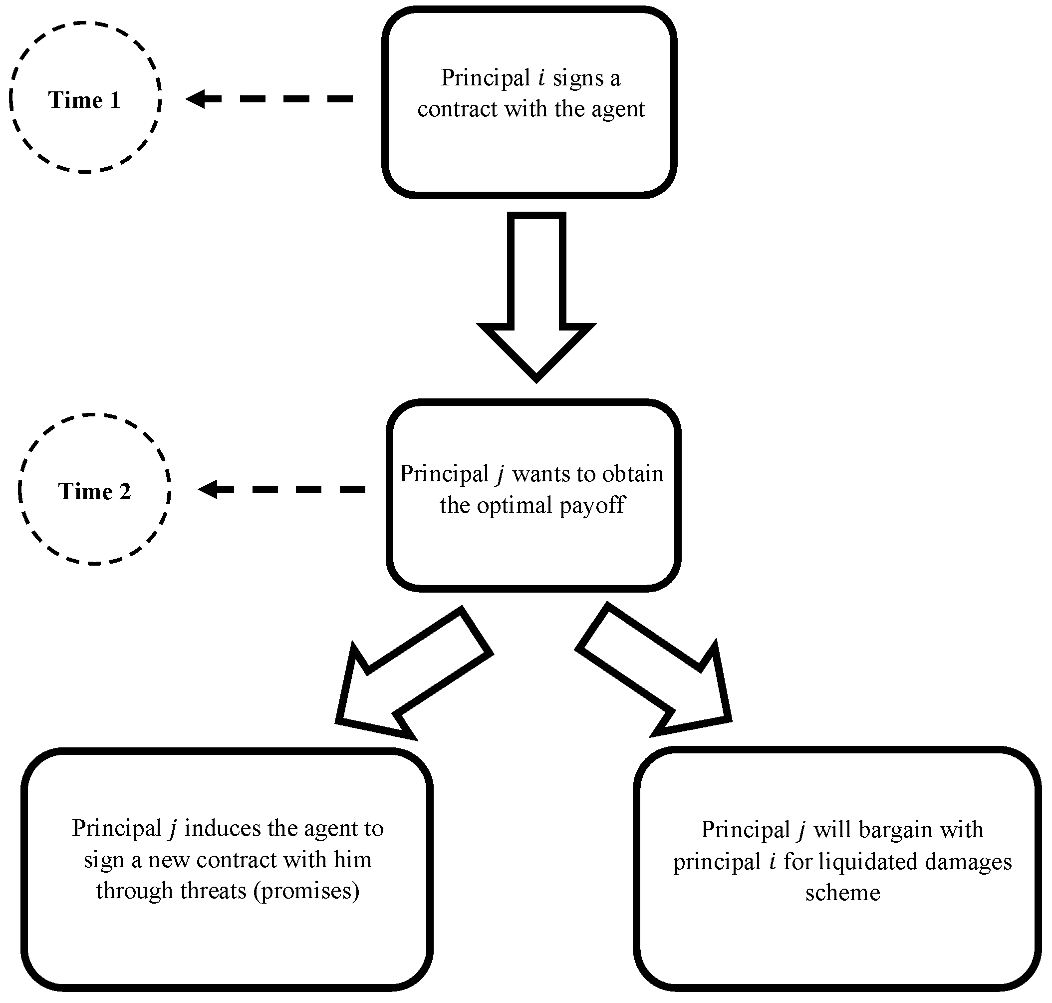
Figure 1 illustrates the entire game and delegation process. First, principal $i$ signs a contract with the agent at time 1. If the agent breaches the contract, they will pay liquidated damages. Second, in order to obtain the optimal payoff at time 2, principal $j$ will persuade the agent to sign a new contract with them and pay LDs to principal $i$ (We use a vivid metaphor: “poaching” and “job-hopping” process. Whether the principal $j$ can successfully “poach” (or whether the agent is willing to “job-hop”) depends on whether the principal $j$ can provide the agent with sufficient “job-hopping” incentives). Meanwhile, principal $j$ will negotiate with principal $i$ regarding LDs until a mutually satisfactory LDs scheme arises.

We show the optimal contract between principal $i$ and the agent, and how LDs affect the optimal contract in Proposition 1. We analyze the game process among principal $j$, principal $i$, and agent at time 2 in the following paragraphs.

First of all, it is important to note that our assumptions are within the context of a zero-sum game. There is only one agent, and they can only sign a contract with one principal at a time. That means if they sign a contract with one principal, the other principal will receive zero payoff. Therefore, principal $j$ needs to persuade the agent to break the contract and sign a new contract with them.

In order to obtain the optimal payoff, at time 2, principal $j$ will try to persuade the agent to join them. Figure 2 shows the process of principal $j$’s persuasions of the agent. The game is divided into four stages. In the first stage, principal $j$ has two choices: resistance or non-resistance. If principal $j$ chooses non-resistance, the payoff between principal $j$ and the agent would be $\left(0,{\mathcal{U}}^i\right)$; if principal $j$ chooses to resist, they would pay the resistance cost $g\in {ℝ}^{+}$. In the second stage, principal $j$ uses threats to impose a fixed cost $z\in \begin{array}{c}{ℝ}^{+}-\left\{0\right\}\end{array}$ on the agent. In the third stage, the agent faces two choices: acceptance of the requirements from principal $j$ at the second stage or rejecting them. If the agent accepts, the payoff between principal $j$ and the agent will be $\left({\Pi }^{j^{*}}-g, {\mathcal{U}}^j{}^{*}\right)$, where ${\Pi }^{j^{*}}={\Phi }^j-h{\Phi }^i$ and ${\mathcal{U}}^j{}^{*}=C{E}^j-h{\Phi }^i$ represents the optimal net payoff of principal $j$ and the agent, respectively. If the agent rejects, the game process goes to the fourth stage. In the fourth stage, principal $j$ chooses to act to fulfil their threat or to give up. If principal $j$ chooses action, they will pay corresponding action costs $v\in {ℝ}^{+}$. Therefore, when the agent chooses rejection at the third stage and principal $j$ chooses to take action at the fourth stage, the payoffs of both parties are $\left({\Pi }^{j^{*}}-v-g, {\mathcal{U}}^j{}^{*}-z\right)$. In addition, if principal $j$ wants to sign a contract with the agent, they need to pay LDs to principal $i$. When the agent chooses to reject and principal $j$ chooses to give up, the final payoff would be $\left(-g, 0\right)$. By taking action, principal $j$ forces the agent to sign a contract with them. Since an agent can only have one contract at a time, the agent should first withdraw from the contract signed with principal $i$ and pay LDs before completing the contract with principal $j$. We summarize the results from the above game with Proposition 2.

Proposition 2.

The agent will ultimately choose acceptance if the following conditions are met:$\left\{\begin{array}{c}{\Pi }^{j^{*}}>g\\ {\mathcal{U}}^j{}^{*}>{\mathcal{U}}^i\end{array}\right.$.

Proof. 

See Appendix A.2. □

Two important implications can be obtained from Proposition 2. First, if the cost of resistance is too large, namely ${\Pi }^{j^{*}}<g$, it will cause principal $j$ to lose incentives. As long as the principal can create a large resistance cost, it can ensure that other principals choose non-resistance. Second, the agent wants principal $j$ to provide a sufficiently high-risk subsidy for the default. That is, the net payoff received by the agent from principal $j$ is higher than that received by the agent from principal $i$. When principal $j$ and the agent come to an agreement, the agent will choose to default on their contract with principal $i$. Principal$j$ will pay LDs to principal $i$.

We thus describe the game between principal $i$ and principal $j$. Considering the Nash equilibrium in case 2 and substituting $q=q^i+q^j$, $i=1, 2$, and $i\ne j$ into the contract signed between the agent and principal $j$, we can obtain the following program:

$$\left\{\begin{array}{c}\underset{\left\{q^j, w^j\right\}}{\max }\left\{\beta q^j-w_0^j-w^j{b}_i{q}^j-g-v-h\left(\beta \left(q-q^j\right)-w_0^i-w^i{b}_i\left(q-q^j\right)\right)\right\}\\ s.t. IR: w_0^j+w^j{b}_i{q}^j-\frac{1}{2}c{\left(q^j\right)}^2-\frac{1}{2}\lambda {\left(w^j\right)}^2\sigma \ge 0\\ IC: q^j\in \underset{{\tilde{q}}^j}{\mathrm{argmax}}\left\{w_0^j+w^j{b}_i{\tilde{q}}^j-\frac{1}{2}c{\left({\tilde{q}}^j\right)}^2-\frac{1}{2}\lambda {\left(w^j\right)}^2\sigma \right\}\end{array} \right.$$

(2)

Proposition 3.

The optimal wage contract is given by$\left(q^{j^{*}}\left(h\right), w^{j^{*}}\left(h\right)\right)$only if the condition$h\in \left(\frac{\beta }{cq-\beta }, \frac{c\lambda \sigma +b_i^2}{b_i^2}\right)$is satisfied.

Proof. 

See Appendix A.3. □

Proposition 1 states that there is an optimal contract within the LDs coefficient range $h\in \left(\frac{\beta }{cq-\beta }, \frac{c\lambda \sigma +b_i^2}{b_i^2}\right)$. The value of $h$ is positively related to the output $q^{j^{*}}$, basic wage $w_0^{j^{*}}$, and performance wage $w^{j^{*}}$. Therefore, a change in $h$ will not only affect the output of the principal, but also affect the net payoff of the agent. $h$ is the key coefficient that can affect the whole contract.

Whether the agent can sign a new contract with principal $j$ depends on whether principal $i$ accepts the LDs proposed by principal $j$. Therefore, principal $i$ and principal $j$ form a bargaining game (It is an offer-counter-offer process). Principal $i$ and $j$ need to negotiate an LD to make sense.

Principal $j$ offers principal $i$ an LD scheme. Principal $i$ chooses to accept or reject it. If principal $i$ chooses to accept it, the game ends; if principal $i$ chooses to reject, principal $i$ will put forward a new LD scheme in the next stage, and then principal $j$ chooses to accept or reject it; if principal $j$ chooses to accept, the game ends. If principal $j$ chooses to reject it, principal $j$ will continue to propose another LD scheme, and so on. Therefore, ${\Phi }^j-h_t{\Phi }^i$ represent the net output of principal $j$ and $h_t{\Phi }^i$ represents the net output of principal $i$. $h_t{\Phi }^{ii}$ and ${\Phi }^{ji}-h_t{\Phi }^{ii}$ are the outputs of principal $i$ and principal $j$ when principal $i$ offers the LD scheme, respectively; $h_t{\Phi }^{ij}$ and ${\Phi }^{jj}-h_t{\Phi }^{ij}$ are the outputs of principal $i$ and principal $j$ when principal $j$ offers the LD scheme, respectively. Suppose the discount factor of principal $i$ and principal $j$ is ${\delta }^i\in \left[0, 1\right]$ and ${\delta }^j\in \left[0, 1\right]$, respectively. If the game ends at period $t\in T$, where $t$ is principal $j$’s bid stage, the payoff discount value of principal $j$ is ${\psi }^j={\left({\delta }^j\right)}^{t-1}\left({\Phi }^{jl}-h_t{\Phi }^{il}\right)$, $l=i, j$; the payoff discount value of principal $i$ is ${\psi }^i={\left({\delta }^i\right)}^{t-1}{h}_t{\Phi }^{il}$, $l=i, j$. Figure 3 shows the bargaining game.

We first consider a two-stage bargaining game $T=2$. In the second stage, principal $j$ proposes an LD scheme: $h_2{\Phi }^{ij}$. Principal $i$ will accept because they have no ability to reject. Therefore, principal $j$’s payoff ${\Phi }^{jj}-h_2{\Phi }^{ij}$ in stage 2 is equivalent to their payoff ${\delta }^j\left({\Phi }^{jj}-h_2{\Phi }^{ij}\right)$ in stage 1. If principal $i$ proposes the LD scheme $h_1{\Phi }^{ii}\ge {\delta }^j\left({\Phi }^{jj}-h_2{\Phi }^{ij}\right)$ in the first stage, principal $j$ will choose to accept it. The subgame perfect Nash equilibrium is $\left({\delta }^j\left({\Phi }^{jj}-h_2{\Phi }^{ij}\right), {\Phi }^{ji}-{\delta }^j\left({\Phi }^{jj}-h_2{\Phi }^{ij}\right)\right)$. Considering another three-stage bargaining game $T=3$, in the last stage, principal $i$ proposes an LD scheme: $h_3{\Phi }^{ii}$. Principal $j$ will accept because they have no ability to reject. Therefore, principal $i$’s payoff $h_3{\Phi }^{ii}$ in stage 3 is equivalent to their payoff ${\delta }^i{h}_3{\Phi }^{ii}$ in stage 2. If principal $j$ proposes the LD scheme $h_2{\Phi }^{ij}\ge {\delta }^i{h}_3{\Phi }^{ii}$ in the second stage, principal $i$ will accept. The payoff of principal $j$ is ${\Phi }^{jj}-h_3{\Phi }^{ij}$. In other words, if principal $i$ proposes an LD scheme $h_1{\Phi }^{ii}\ge {\delta }^j\left({\Phi }^{jj}-{\delta }^i{h}_3{\Phi }^{ii}\right)$ in the first stage, principal $j$ will accept. The subgame perfect Nash equilibrium is $\left({\delta }^j\left({\Phi }^{jj}-{\delta }^i{h}_3{\Phi }^{ii}\right), {\Phi }^{ji}-{\delta }^j\left({\Phi }^{jj}-{\delta }^i{h}_3{\Phi }^{ii}\right)\right)$.

Theorem 1.

$T<\infty$, there exists infinite subgame perfect Nash equilibriums in the bargaining game under the common agent situation in two situations:

• If$T=2t+1$, the subgame perfect Nash equilibrium is$\left({\left(-1\right)}^t{\left({\delta }^i{\delta }^j\right)}^{t-1}\left(h_{2t-1}{\Phi }^{ii}{\delta }^i{\delta }^j-\frac{{\delta }^i{\left({\delta }^j\right)}^2{\Phi }^{jj}}{1+{\delta }^i{\delta }^j}\right)+\frac{{\Phi }^{jj}}{1+{\delta }^i{\delta }^j}, {\Phi }^{ji}-{\left(-1\right)}^t{\left({\delta }^i{\delta }^j\right)}^{t-1}\left(h_{2t-1}{\Phi }^{ii}{\delta }^i{\delta }^j-\frac{{\delta }^i{\left({\delta }^j\right)}^2{\Phi }^{jj}}{1+{\delta }^i{\delta }^j}\right)-\frac{{\Phi }^{jj}}{1+{\delta }^i{\delta }^j}\right)$;
• If$T=2t$, the subgame perfect Nash equilibrium is$\left({\left(-1\right)}^t{\left({\delta }^i{\delta }^j\right)}^{t-1}\left({\delta }^j{h}_{2t-2}{\Phi }^{ij}-\frac{{\delta }^i{\left({\delta }^j\right)}^2{\Phi }^{jj}}{1+{\delta }^i{\delta }^j}\right)+\frac{{\Phi }^{jj}}{1+{\delta }^i{\delta }^j}, {\Phi }^{ji}-{\left(-1\right)}^t{\left({\delta }^i{\delta }^j\right)}^{t-1}\left({\delta }^j{h}_{2t-2}{\Phi }^{ij}-\frac{{\delta }^i{\left({\delta }^j\right)}^2{\Phi }^{jj}}{1+{\delta }^i{\delta }^j}\right)-\frac{{\Phi }^{jj}}{1+{\delta }^i{\delta }^j}\right)$

Proof. 

See Appendix A.4. □

Theorem 1 shows important implications: when principal $i$ puts forward the LD scheme at the last stage, that is, $t=1, 3, 5, 7, \dots$, the LD coefficient $h_{2t-1}$ presents a positive relationship with the net payoff of principal $i$. Therefore, when principal $i$ puts forward the liquidated damage scheme at the last stage, they will increase the coefficient $h_{2t-1}$ value to maximize their net payoff. Similarly, when principal $j$ puts forward the LD scheme at the last stage, that is, $t=2, 4, 6, 8, \dots$, the LD coefficient $h_{2t-2}$ presents a negative relationship with the net payoff of principal $j$. Therefore, when principal $j$ puts forward the LD scheme at the last stage, they will lower the coefficient $h_{2t-2}$ value to maximize their net payoff.

When principal $j$ proposes the LD scheme at the last stage, the LD coefficient they propose will be $h_{2t-2}\in \left(\frac{\beta }{cq-\beta }, \frac{c\lambda \sigma +b_i^2}{b_i^2}\right)$. This liquidated damage coefficient ensures the maximization of payoffs from their new contract with the agent (see Proposition 1). Moreover, this LD coefficient also influences the agent’s performance wage. However, when principal $i$ proposes the LD scheme at the last stage, the LD coefficient they propose may be not in the range: $h_{2t-1}\in \left(\frac{\beta }{cq-\beta }, \frac{c\lambda \sigma +b_i^2}{b_i^2}\right)$. Under this situation, for principal $j$, the LD proposed by principal $i$ will affect their contract with the agent, even though they have to accept such an LD scheme (because it is a subgame perfect Nash equilibrium result). According to the Proposition 1, such results will have a significant impact on the agent’s optimal payoff. Therefore, in the $T=2t+1$, for principal $j$, how to formulate the LD scheme such that $h_{2t-1}\in \left(\frac{\beta }{cq-\beta }, \frac{c\lambda \sigma +b_i^2}{b_i^2}\right)$ proposed by principal $i$ is a problem to be solved. In other words, motivating principal $i$ to propose the LD scheme $h_{2t-1}\in \left(\frac{\beta }{cq-\beta }, \frac{c\lambda \sigma +b_i^2}{b_i^2}\right)$ is the problem that principal $j$ needs to think about. We first present the following corollary to prove that when $\forall h_{2t-1}\in \left(\frac{\beta }{cq-\beta }, \frac{c\lambda \sigma +b_i^2}{b_i^2}\right)$, there is a unique subgame perfect Nash equilibrium in the bargaining game.

Corollary 1.

When $\forall \lambda \in \left(-\infty ,-\frac{4b_i^2}{c\sigma }\right)$, there exists a unique subgame perfect Nash equilibrium in the bargaining game under a common agent, if the following conditions are satisfied:

• ${\Phi }^{ii}{\delta }^i={\Phi }^{ij}$;
• ${\Phi }^{ii}\in \left(-\frac{1}{{\left({\delta }^i{\delta }^j\right)}^t}, \frac{1}{{\left({\delta }^i{\delta }^j\right)}^t}\right)$

Proof. 

See Appendix A.5. □

Through proof of Corollary 1, $h_{2t-1}=h_{2t-2}\in \left(\frac{\beta }{cq-\beta }, \frac{c\lambda \sigma +b_i^2}{b_i^2}\right)$ can be obtained by ensuring that principal $i$’s net payoff when principal $i$ proposes the LD scheme is equal to the present value of their net payoff $\frac{{\Phi }^{ij}}{{\delta }^i}$: The corollary further states the uniqueness of the subgame perfect Nash equilibrium on the basis of Theorem 1. Since the domain is $ℝ$, there is a conjecture that $\forall h_t\in \left(0, \frac{\beta }{cq-\beta }\right)\bigcup \left(\frac{c\lambda \sigma +b_i^2}{b_i^2},+\infty \right)$, $\exists \xi : \left(0, \frac{\beta }{cq-\beta }\right)\bigcup \left(\frac{c\lambda \sigma +b_i^2}{b_i^2},+\infty \right)⟶\left(\frac{\beta }{cq-\beta }, \frac{c\lambda \sigma +b_i^2}{b_i^2}\right)$. The mapping $\xi$ essentially shifts $h_t$ into $\left(\frac{\beta }{cq-\beta }, \frac{c\lambda \sigma +b_i^2}{b_i^2}\right)$. Therefore, the existence of the mapping means that the following assertion can be created.

Corollary 2.

When$\forall h_t\in \left(\frac{\beta }{cq-\beta }, \frac{c\lambda \sigma +b_i^2}{b_i^2}\right)$, the infinite subgame perfect Nash equilibrium in the bargaining game under a common agent is Pareto optimal.

Proof. 

See Appendix A.6. □

Theorem 2.

Let$\mathcal{D}=\left(\frac{\beta }{cq-\beta }, \frac{c\lambda \sigma +b_i^2}{b_i^2}\right)$. There is a mechanism$\xi$, such that a unique subgame perfect Nash equilibrium in the bargaining game under a common agent situation exists, if$\xi$is a bounded linear operator and bijection.

Proof. 

See Appendix A.7. □

Figure 4 shows the path of the mapping of principal $i$. If principal $i$’s LD coefficient is not in the scope of principal $j$’s optimal LD coefficient, principal $j$ will enable the mechanism to ensure that principal $i$’s LD coefficient is within the expected range. After that, both participants will reach an agreement in $p^{*}$ through mapping ${\varsigma }_2$ (Principal $j$ can obtain the payoff in the subgame Nash equilibrium through the mapping ${\varsigma }_2$). The process by which principal $i$ reaches a subgame Nash equilibrium is essentially a complex mapping $\mathcal{H}={\varsigma }_2\circ \xi$. Thus, we need to use a mechanism $\xi$ that causes principal $i$ to believe that principal $j$’s optimal LD coefficient is at least as good as other LD coefficients. Therefore, we prove homeomorphism between $\mathcal{D}$ and ${\mathcal{D}}^c$ by Theorem 2.

Theorem 2 is a further complement to Theorem 1. We find that for principal $i$, after the introduction of the mechanism $\xi$, their LD scheme is the same as principal $j$’s in topological property. In fact, $\xi$ is a mechanism to ensure that the LD coefficient proposed by principal $i$ (the first mover) is in agreement with that proposed by principal $j$, because for any situation where $h_t>0$, the first-mover always has an incentive to put forward a scheme (see Proposition 1). The late-mover must devise a mechanism to force the first-mover to act in accordance with the late-mover’s LD scheme.

Theorem 2 ensures that there is a mechanism such that the principal has an incentive to choose $h_t\in \left(\frac{\beta }{cq-\beta }, \frac{c\lambda \sigma +b_i^2}{b_i^2}\right)$. Combined with Corollary 2, we can conclude that only when $h_t\in \left(\frac{\beta }{cq-\beta }, \frac{c\lambda \sigma +b_i^2}{b_i^2}\right)$ can the LD generate the Pareto optimal solutions to solve the principal–principal conflicts under common agency.

We have completed the discussion of the whole process presented in Figure 1 under the condition of complete information. We discuss how the liquidated damage mechanism affects the optimal contract and principal–principal conflicts in the case of a common agent. In the Section 3, we will discuss the effect of the liquidated damage mechanism under incomplete information on the optimal contract in the case of a common agent.

2.2. Modeling under Incomplete Information

We assume that the agent’s real risk aversion $\widehat{\lambda }\in \left[\underset{\_}{\lambda }, \overline{\lambda }\right]=\mathcal{A}$ is private information, where $\overline{\lambda }$ is the upper bound of $\widehat{\lambda }$ and $\underset{\_}{\lambda }$ is the lower bound of $\widehat{\lambda }$. The principals do not know the real risk aversion of agent, only its distribution function $F_a\left(\lambda \right)$ and probability density function $f_a\left(\lambda \right)$. We assume that principal $i$’s real type $\widehat{\rho }\in \left[\underset{\_}{\rho }, \overline{\rho }\right]=\mathcal{P}$ is private information to principal $j$. Principal $j$ does not know the real type of principal $i$, only its distribution function $F_p\left(\rho \right)$ and probability density function $f_p\left(\rho \right)$. For agents, the real type of principals is public information [26].

Reconsider Figure 1. At time 1, principal $i$ signs a contract with the agent and due to the incomplete information, program (1) can be changed to the following (following the method from [26]):

$$\left\{\begin{array}{c}\underset{\left\{q^i, w^i\right\}}{\max }\left\{\beta q^i-w_0^i\left(\lambda \right)-w^i\left(\lambda \right)b_i{q}^i+{\Phi }^i\max \left\{0, h\right\}\right\}\\ s.t. IR: w_0^i\left(\lambda \right)+w^i\left(\lambda \right)b_i{q}^i-\frac{1}{2}c{\left(q^i\right)}^2-\frac{1}{2}\lambda {\left(w^i\left(\lambda \right)\right)}^2\sigma -{\Phi }^i\max \left\{0, h\right\}\ge 0\\ IC: q^i\in \underset{{\tilde{q}}^i}{\mathrm{argmax}}\left\{w_0^i\left(\lambda \right)+w^i\left(\lambda \right)b_i{\tilde{q}}^i-\frac{1}{2}c{\left({\tilde{q}}^i\right)}^2-\frac{1}{2}\lambda {\left(w^i\left(\lambda \right)\right)}^2\sigma -{\Phi }^i\max \left\{0, h\right\}\right\}\end{array} \right.$$

(3)

When $h>0$, substituting $q^i=\frac{\left(1+h\right)w^i{b}_i-h\beta }{c}$ into IR, let $U\left(\lambda , \widehat{\lambda }\right)\equiv \left(1+h\right)w_0^i\left(\widehat{\lambda }\right)+\frac{{\left(1+h\right)}^2{\left(w^i\left(\widehat{\lambda }\right)\right)}^2{b}_i^2-\left(1+h\right)b_{i}h{w}^i\left(\widehat{\lambda }\right)\beta }{c}-\frac{{\left(\left(1+h\right)w^i\left(\widehat{\lambda }\right)b_i-h\beta \right)}^2}{2c}-\frac{1}{2}\lambda {\left(w^i\left(\widehat{\lambda }\right)\right)}^2\sigma -\frac{h\beta \left(1+h\right)w^i\left(\widehat{\lambda }\right)b_i-h^2{\beta }^2}{c}$, and $U\left(\lambda \right)\equiv U\left(\lambda , \lambda \right)$, we introduce the Lemma 1 (Meng and Tian, 2013):

Lemma  1.

The surplus function$U\left(\lambda \right)$and performance wage function$w^i\left(\lambda \right)$are implementable ([26] explained convex in detail: “Defining the convex functions is through representing them as maximum of affine functions, that is,$s\left(x\right)$is convex if and only if$s\left(x\right)=\underset{a, b\in \Omega }{\max }\left(a\cdot x+b\right)$, for some$a\in {ℝ}^n, b\in ℝ$and some$\Omega \subset {ℝ}^{n+1}$″). if and only if:

• Envelop condition$U^{\prime }\left(\lambda \right)=\frac{1}{2}{\left(w^i\right)}^2\sigma$is satisfied;
• $U\left(\lambda \right)$is convex in$\lambda$.

Proof. 

See Appendix B.1. □

Substituting $U\left(\lambda \right)$ into the ${\Pi }^i$, we get:

$$\begin{gathered} {\Pi }^i={{\displaystyle \int }}_{\underset{\_}{\lambda }}^{\overline{\lambda }}\left[\beta q^i-w_0^i\left(\lambda \right)-w^i\left(\lambda \right)b_i{q}^i+h{\Phi }^i\right]f_a\left(\lambda \right)d\lambda \\ ={{\displaystyle \int }}_{\underset{\_}{\lambda }}^{\overline{\lambda }}\left[\beta \frac{\left(1+h\right)w^i\left(\lambda \right)b_i-h\beta }{c}-\frac{1}{2}c{\left(\frac{\left(1+h\right)w^i\left(\lambda \right)b_i-h\beta }{c}\right)}^2 \\ -\frac{1}{2}\lambda {\left(\frac{\left(1+h\right)w^i\left(\lambda \right)b_i-h\beta }{c}\right)}^2\sigma -U\left(\lambda \right)\right]f_a\left(\lambda \right)d\lambda \end{gathered}$$

Thus, based on the Lemma 1, the program (3) can be changed to the following form:

$$\left\{\begin{array}{c}\underset{U\left(\lambda \right), w^i\left(\lambda \right)}{\max }\left\{{{\displaystyle \int }}_{\underset{\_}{\lambda }}^{\overline{\lambda }}\left[\beta \frac{\left(1+h\right)w^i\left(\lambda \right)b_i-h\beta }{c}-\frac{1}{2}\left(c-\lambda \sigma \right){\left(\frac{\left(1+h\right)w^i\left(\lambda \right)b_i-h\beta }{c}\right)}^2-U\left(\lambda \right)\right]f_a\left(\lambda \right)d\lambda \right\}\\ s.t. U\left(\lambda \right)\ge 0\\ U^{\prime }\left(\lambda \right)=\frac{1}{2}{\left(w^i\right)}^2\sigma \end{array}\right.$$

(4)

We summarize the optimal solution of program (4) as follows:

Proposition 4.

When default occurs, there exists an optimal contract$\left(q^{i^{*}}\left(\lambda ;h\right), w^{i^{*}}\left(\lambda ;h\right)\right)$under unobservable risk aversion of the agent, if$\lambda \in \left(\frac{c}{\sigma },+\infty \right)$.

Proof. 

See Appendix A.8. □

Proposition 4 implies another condition: $\lambda \in \left(\frac{c}{\sigma },+\infty \right)$. The common feature of Proposition 1 and 4 is that the LD coefficient significantly affects output and performance wage. However, Proposition 3 requires more stringent conditions. Under incomplete information, the optimal contract between principal $i$ and the agent should be based on the risk-seeking type of agent. This means that the agent needs to have greater tolerance for risk under an incomplete information situation.

At time 2, principal $j$ will start a game with the agent under the condition of incomplete information. Before analyzing this game, we first need to analyze the types of agents. If principal $j$ finally forces the agent to cancel the contract with principal $i$ and sign a new contract, under incomplete information, principal $j$ and the agent obtain the optimal contract through the following planning:

$$\left\{\begin{array}{c}\underset{\left\{q^j, w^j\right\}}{\max }\left\{\beta q^j-w_0^j\left(\lambda \right)-w^j\left(\lambda \right)b_i{q}^j-g-v-h\left(\beta \left(q-q^j\right)-w_0^i\left(\lambda \right)-w^i\left(\lambda \right)b_i\left(q-q^j\right)\right)\right\}\\ s.t. IR: w_0^j\left(\lambda \right)+w^j\left(\lambda \right)b_i{q}^j-\frac{1}{2}c{\left(q^j\right)}^2-\frac{1}{2}\lambda {\left(w^j\left(\lambda \right)\right)}^2\sigma -d\ge 0\\ IC: q^j\in \underset{{\tilde{q}}^j}{\mathrm{argmax}}\left\{w_0^j\left(\lambda \right)+w^j\left(\lambda \right)b_i{\tilde{q}}^j-\frac{1}{2}c{\left({\tilde{q}}^j\right)}^2-\frac{1}{2}\lambda {\left(w^j\left(\lambda \right)\right)}^2\sigma -d\right\}\end{array}\right.$$

(5)

Using Lemma 1, we summarize the optimal contract as the following proposition:

Proposition 5.

If$\lambda \in \left(\frac{c}{\sigma },+\infty \right)$, then there exists an optimal contract$\left(w^{j^{*}}\left(\lambda ;h\right), q^{j^{*}}\left(\lambda ;h\right)\right)$.

Proof. 

See Appendix A.9. □

Proposition 5 shows that only when $\lambda >\frac{c}{\sigma }$ will the optimal contract be generated between principal $j$ and the agent. There is no constraint on $h$ in the necessary conditions of Proposition 4. Therefore, principal $i$ can accept any LD scheme when $\lambda >\frac{c}{\sigma }$. Using Proposition 4, we obtain the possible types of agent in time 2.

Figure 5 shows the game between principal $j$ and the agent under incomplete information. With incomplete information, the game between principal $j$ and the agent transforms into a typical signaling game. Again, in the first stage, principal $j$ has two choices: resistance or non-resistance. If principal $j$ chooses non-resistance, the payoff between principal $j$ and the agent is $\left(0, 0\right)$; if principal $j$ chooses to resist, they will pay a resistance cost $g\in {ℝ}^{+}$. In the second stage, principal $j$ requests a fixed cost $z\in \begin{array}{c}{ℝ}^{+}\end{array}$ from the government to end resistance. However, in the next stage, it is different from the stage in the game we described in Section 2. Nature [27] first chooses the type of agent. Principal $j$ only knows the probability density function $f_a\left(\lambda \right)$ of the agent’s type. The agent then has two signals, rejection or acceptance, while principal $j$ has two choices, action or giving up.

Our other assumptions are the same as in Section 2. In particular, when the agent type is ${\lambda }_1$ and if the principal chooses to take an action, their final payoff will be $\left({\Pi }^{j^1}, {\mathcal{U}}^{j^1}\right)$. Similarity, their final payoff will be $\left({\Pi }^{j^2}, {\mathcal{U}}^{j^2}\right)$, when the agent type is ${\lambda }_2$.

Theorem 3.

There exists a subgame perfect Bayesian Nash equilibrium$\left(\left(end, Resistance\right), Acceptance\right)$, if the following conditions are satisfied:${\mathcal{U}}^i\in \left(0, {\mathcal{U}}^{j^1}\right)\bigcap \left(0, {\mathcal{U}}^{j^2}\right)$.

Proof. 

See Appendix A.10. □

Theorem 3 shows a very important implication: there exists a subgame perfect Bayesian Nash equilibrium under incomplete information, and this equilibrium enables principal $j$ to sign a new contract with the agent. The conditions for ${\mathcal{U}}^i\in \left(0, {\mathcal{U}}^{j^1}\right)\bigcap \left(0, {\mathcal{U}}^{j^2}\right)$ denote that as long as principal $j$ pays a high enough amount to the agent, they will have an incentive to sign a new contract. In other words, the agent has an incentive to “job-hop.” This is important because it means that even though the information is incomplete, the agent can reach an agreement with principal $j$ through the signaling mechanism.

Figure 6 shows the negotiation game between principal $j$ and principal $i$ on the LD scheme. One practical issue we need to emphasize is that the information type for principal $i$ is public information (the reason for this is that principal $j$ learns about principal $i$ through the common agent), while principal $j$’s information is private information. Suppose that the probability of principal $j$ choosing rejection is $F_l\left(M_1\right)$ and the probability of choosing acceptance is $F_l\left(M_2\right)=1-F_l\left(M_1\right)$, $\forall l\in T$. After $2t$ negotiations, the negotiations are entirely completed. According to the sequential equilibrium, if $h_{2t}\left(\rho \right){\Phi }^{ii}>{\Phi }^i$. At stage $2t$, principal $i$ provides a quotation, principal $j$ chooses whether to reject it, and then the game ends. Similar to the situation under perfect information, there exists a subgame perfect Nash equilibrium in the multi-principal negotiation mechanism under incomplete information. We describe it in Theorem 4.

Theorem 4.

There is an optimal liquidated damage$\left\{\begin{array}{c}{\left(h_1\left(\rho \right)\right)}^{i*}, if principal i first quote\\ {\left(h_1\left(\rho \right)\right)}^{j*}, if principal j first quote\end{array}\right.$, such that a sequential equilibrium exists, if the following conditions are satisfied:$f_n^{\prime }\left(\rho \right)<0$,$\forall n\in T$and$f$is a bijection.

Proof. 

See Appendix A.11. □

Theorem 4 proves that there is also an LD scheme which ensures that both sides come to an agreement under incomplete information. The two conditions in Theorem 4 ensure the existence of a maximum and the existence of inverse operators, respectively. We divided the proof of Theorem 4 into two cases: the game ending with principal $i$ and the game ending with principal $j$. These two different situations correspond to two different LDs. The most important reason is that the information of principal $j$ is private to principal $i$, which leads to the need for principal $i$ to guess the action of principal $j$ through the distribution function. Through the backward recursion method, we determine the optimal liquidated damages in the first stage, which means that as long as the LD coefficient provided by principal $i$ (or $j$) in the first stage is not less than ${\left(h_1\left(\rho \right)\right)}^{i*} ($or ${\left(h_1\left(\rho \right)\right)}^{j*}$), principal $j$ (or $i$) will choose to accept. Furthermore, combining Proposition 4, we find that if ${\left(h_1\left(\rho \right)\right)}^{i*}\in \left(\frac{c}{b_i}\sqrt{-\frac{\varsigma \sigma }{c+\lambda \sigma }}-1,+\infty \right)$, principal $j$ will choose to accept the LD scheme at the first stage. However, for principal $i$, there is no constraint at the first stage of the proposed LD scheme, being in the range $\left(\frac{c}{b_i}\sqrt{-\frac{\varsigma \sigma }{c+\lambda \sigma }}-1,+\infty \right)$. Thus, if the negotiation time increases, the negotiation cost will increase. If principal $j$ makes an offer first, since principal $j$ knows principal $i$’s information, principal $j$’s LD scheme in the first stage can make principal $i$ accept. As a result, negotiation costs will be significantly reduced. This means that the negotiation initiated by principal $j$ has a cost advantage. The conclusion of Theorem 4 also implies that LDs can effectively resolve principal–principal conflicts because of the existence of a sequential equilibrium which ensures that both parties reach a consensus agreement. Applying the findings of Corollary 2, there is also a mechanism that enables principal $i$ to choose to accept the scheme in the first stage.

3. Discussion

Our results show that the liquidated damages mechanism is another effective way to resolve multi-principal conflicts compared with decentralization of power.

The main findings of this paper are as follows: firstly, through Propositions 1, 2, 3, and 4, we find that the setting of liquidated damages affects the optimal contract between principals and the agent. The value range of liquidated damages affects whether principals and agents can maximize the payoff. This finding is the premise of our comprehensive study, because only when liquidated damages enter into the contract between principals and agents can this method resolve the principal–principal conflict.

Second, LDs play an essential role in resolving principal–principal conflict. According to theorems 1 and 4, a Nash equilibrium is determined by liquidated damages negotiation between principals. Under the equilibrium, neither principal party will change the quotation strategy for liquidated damages. Although the liquidated damages quotation considered by principal $j$ may not be within the actual price range of principal $i$, we find that principal $i$ can induce principal $j$’s liquidated damages quotation through a mechanism such that the two parties finally reach the Nash equilibrium. The “inducement” is a kind of negotiation ability, in essence. Therefore, the extent to which principal $j$ can “induce” principal $i$ depends on the negotiating power of principal $j$.

The optimal range of the LDs scheme is related to the type of agent and total output. The greater (smaller) the agent’s absolute risk coefficient is, the greater (smaller) the optimal range of the LD coefficient value is. The larger (smaller) the total output is, the smaller (larger) the optimal range of the LD coefficient value is. Regardless of whether the information is symmetric or not, we prove that an optimal LD allows multiple principals and the common agent to agree. The optimal LD scheme effectively resolves multiple principal conflicts. In conclusion, we prove that LD is an effective method to resolve multi-principal conflicts. As we described in the Introduction, our findings complement the work of [25]. Through analyzing the processes of delegation, our findings (Theorem 1, 2, 4 and Corollary 1) are also supported by [25] (p. 941).

The critical role of LD in contracts has been repeatedly verified using legal theory [9,28,29]. We once again prove its importance from the perspective of the principal–agent theory. Ref. [30] confirmed the role of negotiation in resolving principal–principal conflicts. He argued that congressional oversight of bureaucracies has an increasing emphasis on negotiating administrative procedures rather than outcome-based incentives as initially envisaged. Credible commitments from principal agents are also vital. This is consistent with our conclusion analysis: the principal–principal conflict can be resolved by negotiating liquidated damages. We further expand the role of liquidated damages negotiation in principal–principal conflict. LD negotiation can eventually form a Nash equilibrium that satisfies both parties.

The legal theory explains the setting of liquidated damages as follows: LDs are compensation for the injured party’s loss but not a punishment for the breaching party. Therefore, as a general rule, most courts require liquidated damages to be a reasonable estimate of the expected losses when entering into the contract. However, some courts will also consider actual damages to determine whether liquidated damages are reasonable. Some jurisdictions will not enforce the LDs clause, depending on whether or not it is reasonable that the aggrieved party cannot prove that they have suffered at least some actual harm. Since LDs are not punitive, some courts have held that contracts cannot contain clauses that allow aggrieved parties to choose whether to seek actual damages or LDs. These courts held that such clauses penalized the defaulting party and failed to achieve the purpose of agreeing to a penalty, so they limited plaintiffs’ damages to actual losses. These conclusions are consistent with our hypothesis that the LDs act as compensation rather than punishment for the injured party. Thus, we find a Nash equilibrium between the injured and breaching parties. Only from the perspective of compensation can the two parties reach an agreement in the final bargain.

Our findings demonstrate the effectiveness of using the LD mechanism to solve multi-principal problems. We further find reasons in the current literature why the LD mechanism works. LDs allow the breaching party to obtain the residual value of the transaction and limit the non-breaching party’s benefit to the value of the initial contract, making it easier to obtain an effective outcome. In particular, LDs will always lead to an optimal outcome if the parties specify a sufficiently high quantity and a sufficiently low price in the ex ante contract. According to [7]’s hypothesis, the parties involved in the decisions about whether to default and the degree of default are interdependent (the degree of dependence is related to the degree of risk aversion). This is consistent with our findings that a subgame perfect Nash equilibrium exists under perfect information and a sequential equilibrium exists under imperfect information (both parties need to rely on each other’s strategy to perform the following action). Among these findings, there is an important argument: in order to prevent the seller from frequently defaulting (since they will pay very little in damages for default), the buyer can impose penalties in the contract; unless production costs are enormous, this will ensure that the seller has no incentive to default because of sufficient penalty mechanisms. The findings of [8] explain corollary 2 of our paper. This is a mechanism by which parties in breach of contract can agree on liquidated damages. In this conclusion, we emphasize that the mechanism ensures that the old principal does not overcharge. One possible reason comes from [8], where the potential defaulter can influence the probability of finding an alternative buyer. When the defaulter needs more bargaining power, they have little incentive to mitigate default damage. This is because, while the new principal may fully bear negotiation costs, this advantage will be diminished as long as the new principal has some bargaining power.

Our results can be applied to multiple explicit contract scenarios. According to the Pareto effectiveness, we prove that the liquidated damages mechanism can effectively solve the multi-principal conflict problem under common agency. Our findings prove that it is feasible to answer under what conditions an agent’s breach of contract and a principal’s “poaching” behavior are feasible. On the contrary, our conclusion also suggests how to prevent the agent’s breach of contract by signing a new contract with another principal—that is, when $h\notin \left(\frac{\beta }{cq-\beta }, \frac{c\lambda \sigma +b_i^2}{b_i^2}\right)$, the high liquidated damages will force the principal to give up the “poaching” action and prevent the agent’s ex post breach of contract (moral risk).

4. Conclusions

This paper is the first to study liquidated damages in the form of the principal–agent theory combined with a non-cooperative game. LD is another effective form to resolve principal–principal conflict. This paper aimed to prove that LD effectively resolves principal–principal conflicts under common agency. We achieved the research purpose of this paper by solving the three research questions.

We further showed the delegation processes based on [25]. We found that the LD value impacts the contract between principals and agents, which is directly related to whether principals and agents have an optimal contract. We proved that the LD is another way to resolve principal–principal conflict effectively. This is a notable contribution of this paper. We provided new theoretical evidence for the validity of renegotiation. At the same time, our findings can be applied in various situations (such as sports clubs, film and entertainment companies, and other situations involving LDs).

Future research can be conducted as follows: first, the negotiation cost of the principals can be considered. This is a crucial variable that directly affects whether the principal is willing to negotiate (if the cost is too high, the principal will not negotiate). Second, negotiation skills as an essential variable should be studied. This paper assumes that both sides of the game have good negotiation ability, so each participant can complete the game through negotiation. Negotiations that may have resulted in an agreement fail because of one participant’s poor negotiation skills. Third, the LDs can be compared in two information situations and the contract efficiency can be analyzed under different situations.

References

1. Siddharth Gosain, A.C. Player Contracts, Liquidated Damages & The Principle of Reciprocity At FIFA & CAS. 2021. Available online: https://www.lawinsport.com/topics/item/player-contracts-liquidated-damages-the-principle-of-reciprocity-at-fifa-cas#_ftn1 (accessed on 17 November 2021).
2. Grossman, S.J.; Hart, O.D. The Costs and Benefits of Ownership: A Theory of Vertical and Lateral Integration. J. Political Econ. 1986, 94, 691–719. [Google Scholar] [CrossRef] [Green Version]
3. Hart, O.; Moore, J. Incomplete Contracts and Renegotiation. Econometrica 1988, 56, 755–785. [Google Scholar] [CrossRef]
4. Dixit, A.; Grossman, G.M.; Helpman, E. Common Agency and Coordination: General Theory and Application to Government Policy Making. J. Political Econ. 1997, 105, 752–769. [Google Scholar] [CrossRef] [Green Version]
5. Williamson, O.E. Markets and Hierarchies: Analysis and Antitrust Implications: A Study in the Economics of Internal Organization; Free press: New York, NY, USA, 1975. [Google Scholar]
6. Williamson, O.E. The Economic Institutions of Capitalism: Firms, Markets, Relational Contracting; Free Press: New York, NY, USA, 1985. [Google Scholar]
7. Shavell, S. Damage Measures for Breach of Contract. Bell J. Econ. 1980, 11, 466–490. [Google Scholar] [CrossRef]
8. Zhang, F. Dynamic Contract Breach. J. Law Econ. Organ. 2009, 27, 453–484. [Google Scholar] [CrossRef]
9. Edlin, A.; Reichelstein, S. Holdups, Standard Breach Remedies, and Optimal Investment. Am. Econ. Rev. 1996, 86, 478–501. [Google Scholar]
10. Hwang, I.; Li, F. Transparency of outside options in bargaining. J. Econ. Theory 2017, 167, 116–147. [Google Scholar] [CrossRef]
11. Chung, T.-y. On the Social Optimality of Liquidated Damage Clauses: An Economic Analysis. J. Law Econ. Organ. 1992, 8, 280–305. [Google Scholar]
12. Lee, J. Incomplete Information, Renegotiation, and Breach of Contract. Econ. Bull. 2005, 3, 1–7. [Google Scholar]
13. Myerson, R.B.; Satterthwaite, M.A. Efficient mechanisms for bilateral trading. J. Econ. Theory 1983, 29, 265–281. [Google Scholar] [CrossRef] [Green Version]
14. Young, M.N.; Peng, M.W.; Ahlstrom, D.; Bruton, G.D.; Jiang, Y. Corporate Governance in Emerging Economies: A Review of the Principal–Principal Perspective. J. Manag. Stud. 2008, 45, 196–220. [Google Scholar] [CrossRef]
15. Demsetz, H.; Lehn, K. The Structure of Corporate Ownership: Causes and Consequences. J. Political Econ. 1985, 93, 1155–1177. [Google Scholar] [CrossRef]
16. Faccio, M.; Lang, L.H.P.; Young, L. Dividends and Expropriation. Am. Econ. Rev. 2001, 91, 54–78. [Google Scholar] [CrossRef]
17. Ward, D.R.; Filatotchev, I. Principal-principal-agency relationships and the role of external governance. Manag. Decis. Econ. 2010, 31, 249–261. [Google Scholar] [CrossRef]
18. Lin, C.-P.; Chuang, C.-M. Principal-Principal Conflicts and IPO Pricing in an Emerging Economy. Corp. Gov. Int. Rev. 2011, 19, 585–600. [Google Scholar] [CrossRef]
19. Sørensen, R.J. Does Dispersed Public Ownership Impair Efficiency? The Case of Refuse Collection in Norway. Public Adm. 2007, 85, 1045–1058. [Google Scholar] [CrossRef]
20. Khalil, F.; Martimort, D.; Parigi, B. Monitoring a common agent: Implications for financial contracting. J. Econ. Theory 2007, 135, 35–67. [Google Scholar] [CrossRef] [Green Version]
21. Gailmard, S. Multiple Principals and Oversight of Bureaucratic Policy-Making. J. Theor. Politics 2009, 21, 161–186. [Google Scholar] [CrossRef] [Green Version]
22. Suwannasichon, R. Liquidated Damages in Airline Business Employment Contracts. Thammasat Bus. Law J. 2019, 9, 46–62. [Google Scholar]
23. Zhang, Y. Liquidated Damages and Compensation in Labor Contract Law and the Improvement of Its System. In Proceedings of the 2020 International Conference on Economic Management and Social Science (ICEMSS 2020), Nanjing, China, 25–26 April 2020. [Google Scholar]
24. Bai, C.-E.; Mao, W.; Tao, Z. Breach Inducement Activities and Performance of Breach Remedies. SSRN 2020, 3236925. Available online: https://papers.ssrn.com/sol3/papers.cfm?abstract_id=3236925 (accessed on 6 November 2022).
25. Bernheim, B.D.; Whinston, M.D. Common Agency. Econometrica 1986, 54, 923–942. [Google Scholar] [CrossRef]
26. Meng, D.; Tian, G. Multi-task incentive contract and performance measurement with multidimensional types. Games Econ. Behav. 2013, 77, 377–404. [Google Scholar] [CrossRef] [Green Version]
27. Harsanyi, J.C. Bayesian decision theory, subjective and objective probabilities, and acceptance of empirical hypotheses. Synthese 1983, 57, 341–365. [Google Scholar] [CrossRef]
28. Reed, B.B. Liquidated Damages Provisions Strategic Drafting and Enforcement Issues. Franch. Law J. 2018, 37, 523–552. [Google Scholar]
29. Talley, E.L. Contract Renegotiation, Mechanism Design, and the Liquidated Damages Rule. Stanf. Law Rev. 1994, 46, 1195–1243. [Google Scholar] [CrossRef]
30. Miller, G.J. The Political Evolution of Principal-Agent Models. Annu. Rev. Political Sci. 2005, 8, 203–225. [Google Scholar] [CrossRef]
Figure 1. The entire game and delegation process.
Mathematics 11 00442 g001
Figure 2. The process of principal j ’s “poaching” game.
Mathematics 11 00442 g002
Figure 3. The bargaining game between principal i and principal j .
Mathematics 11 00442 g003
Figure 4. Complex mapping path.
Mathematics 11 00442 g004
Figure 5. The game between principal j and the agent under incomplete information.
Mathematics 11 00442 g005
Figure 6. Negotiation game between two principals.
Mathematics 11 00442 g006
Disclaimer/Publisher’s Note: The statements, opinions and data contained in all publications are solely those of the individual author(s) and contributor(s) and not of MDPI and/or the editor(s). MDPI and/or the editor(s) disclaim responsibility for any injury to people or property resulting from any ideas, methods, instructions or products referred to in the content.