Observer-Based PID Control Protocol of Positive Multi-Agent Systems

Abstract

This paper proposes the observer-based proportional-integral-derivative control of positive multi-agent systems. First, a positive observer is constructed for the considered multi-agent systems in terms of a matrix decomposition approach. Then, a novel proportional-integral-derivative protocol framework is proposed based on an improved observer. By using copositive Lyapunov function, the positivity and consensus of the multi-agent systems are achieved. The corresponding observer and control protocol gain matrices are designed in terms of linear programming. Moreover, the proposed design is developed for heterogeneous positive multi-agent systems. The main contributions of this paper include the following: (i) A positive observer is constructed to estimate the states of positive multi-agent systems; (ii) A novel observer-based proportional-integral-derivative protocol is designed to handle the consensus problem of positive multi-agent systems; and (iii) The presented conditions are solvable in terms of linear programming and the gain matrices can be constructed based on a matrix decomposition technology. Finally, two illustrative examples are provided to verify the effectiveness of the design.

1. Introduction

Multi-agent systems (MASs) have drawn much attention due to their wide application in power engineering [1,2], manufacturing systems [3], robotics [4,5,6], energy systems [7,8], and so on. One of the crucial challenges of MASs is the consensus problem, which means that all agents reach an agreement or cooperate to accomplish a task. Many efforts have been devoted to the consensus issues of MASs, including finite-time consensus [9], event-triggered consensus [10], cluster consensus [11], etc. In real world, there exists a class of MASs with nonnegative variables. Such a class of MASs is called positive MASs (PMASs) [12,13]. They have extensive applications in multiple vehicle systems [14], wireless sensor network [15], COVID-19 transmission process [16], and so on. It is worth noting that the research of PMASs is more complicated than general MASs (non-positive). Few efforts are devoted to PMASs though there have been some significant results on positive systems [17,18,19,20,21]. When dealing with the consensus of PMASs, the designed protocol must take the positivity constraint into consideration in addition to maintaining the convergence of the consensus errors. Therefore, existing approaches to MASs cannot be directly applied to PMASs.

There are many significant control approaches in literature such as fuzzy controller [22], adaptive controller [23], proportional controller [24], proportional-integral controller [25], proportional-derivative controller [26], and proportional-integral-derivative controller [27]. Proportional-integral-derivative (PID) controller is extensively used in various industry processes due to its straightforward and easy-to-understand structure compared to sophisticated controllers [28]. There have been a great amount of interesting findings about PID controllers. In [29], the classical PID control was investigated for high-order affine-nonlinear uncertain systems. Such kind of approach can govern the nonlinear uncertain systems semi-globally without the need for system structures with particular properties like normal or triangular forms. A PID controller for the stabilization of time-delay systems was constructed in [30] by considering all the controller gain matrices and delays as free parameters. The literature [31] proposed a PID controller design strategy based on the adaptive updating rules and data-driven techniques. In addition to the aforementioned systems, PID controllers are frequently employed in MASs. To handle the containment control of heterogeneous high-order MASs, a fully-distributed PID control was investigated in [32]. In [33], an $l_2$ robust PID-like output-feedback control was proposed. By transforming the consensus problem of MASs into the stabilization problem, the consensus of MASs with time-delay was achieved by virtue of the distributed PID controller [34]. In [35], distributed adaptive protocols were designed for nonlinear MASs to handle the distributed consensus problem. The literature [36] investigated the consensus of homogeneous MASs. Multiple fractional-order positive systems were taken into consideration in [37] and the consensus of systems was addressed by means of spectral graph theory. It has been shown that the PID controller has a positive impact on the system performances compared with other control technologies [38]. However, most of existing works on PMASs are devoted to the proportional control or proportional-integral control. Few results focus on the PID control of PMASs. Hence, it is significant to investigate the appropriate PID control of PMASs.

The state of the systems are assumed to be measurable in all the aforementioned literature. In practice, it is difficult to measure all states due to the high cost and technical constraint. As a result, an observer is introduced for the state and the corresponding observer-based control has been extensively considered. To cope with the consensus issue of MASs with directed communication topology, an observer-type protocol was constructed in [39] based on the relative outputs of neighboring agents. In [40], the cooperative output regulation problem of MASs was investigated based on the adaptive distributed observer approach. A proportional integral observer control protocol was constructed in [41] for nonlinear MASs with unknown inputs. For PMASs with undirected communication topology, the literature [42] provided an observer-type dynamic output-feedback protocol. An observer-based consensus protocol was presented in [43] for PMASs with nonlinear control input. In [44], the robust and non-fragile consensus problem of PMASs was investigated by using an observer-based dynamic output-feedback protocol. Fractional-order PMASs were also considered in [45].

This paper investigates the observer-based consensus protocol of PMASs. First, a positive observer is constructed to estimate the states of PMASs. The observer can be used to give the lower and upper boundaries of the real states. Second, a PID control protocol is proposed based on an improved observer. By using copositive Lyapunov functions, the positivity and consensus of PMASs can be guaranteed under the designed observer-based PID protocol. The designed protocol can be generalized for heterogeneous PMASs. The main contributions of this paper include the following: (i) A positive observer for PMASs is constructed; (ii) A novel observer-based PID protocol framework is designed; and (iii) Matrix decomposition technology is used to construct the gain matrices and linear programming is employed to handle the proposed conditions. The remainder of this paper is structured as follows: Preliminaries on positive systems and graph theory are introduced in Section 2. Section 3 shows the main results of positive observer problem and observer-based PID control synthesis. In Section 4, two numerical examples are given to illustrative correctness of the design. The article is concluded in Section 5, which also discusses some potential future research directions.

Notations. In this paper, we denote $\mathbb{R},{\mathbb{R}}^n$ and ${\mathbb{R}}^{m\times n}$ as the sets of real numbers, n-dimensional vectors and the space of $m\times n$ matrices, respectively. Denote $a_{ij}$ as the ith row and jth column entry of matrix A. Matrix $I_n$ denotes the identity matrix with order n. ${\mathbf{1}}_n$ is the ${\mathbb{R}}^n$ column vector with all elements being 1, and ${\mathbf{1}}_n^{\left(ı\right)}$ means the column vector with ıth entry is 1 and other elements are all 0, i.e., ${\mathbf{1}}_n={(\underset{n}{\underbrace{1,1,\cdots ,1}})}^{\top }$ and ${\mathbf{1}}_n^{\left(ı\right)}={(\underset{ı-1}{\underbrace{0,\cdots ,0}},1,\underset{n-ı}{\underbrace{0,\cdots ,0}})}^{\top }$. For a given vector $v\in {\mathbb{R}}^n,v\succ 0(⪰0)$ means that $v_i>0(\ge 0),i=1,2,\cdots ,n$. Similarly, for a matrix $A\in {\mathbb{R}}^{m\times n},A\succ 0(⪰0)$ means that $a_{ij}>0(\ge 0)$. Given matrices $A,B\in {\mathbb{R}}^{m\times n},A\succ B(A⪰B)$ means that $a_{ij}>b_{ij}(a_{ij}\ge b_{ij})$. The notation ⊗ denotes the Kronecker product.

2. Preliminaries

2.1. Positive Theory

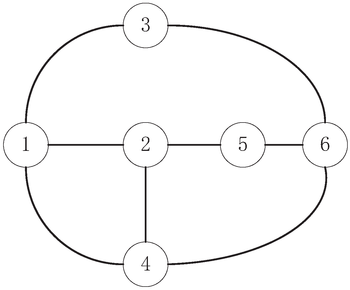
Consider the discrete-time system:

$$\begin{array}{c}x(k+1)=Ax\left(k\right)+Bu\left(k\right),\hfill \\ y\left(k\right)=Cx\left(k\right),\hfill \end{array}$$

(1)

where $x\left(k\right)\in {\mathbb{R}}^s$, $y\left(k\right)\in {\mathbb{R}}^q$, and $u\left(k\right)\in {\mathbb{R}}^m$ denote the system state, output, control input, respectively. Assume that the system matrices satisfy $A⪰0,B⪰0,C⪰0$.

Definition 1

([46,47]). System (1) is said to be positive if and only if for any non-negative initial state and non-negative input, $x\left(k\right)⪰0$ and $y\left(k\right)⪰0$ hold for all $k\in \mathbb{N}$.

Lemma 1

([46,47]). System (1) is positive if and only if $A,B,C$ are non-negative.

Lemma 2

([46,47]). If system (1) is positive, then the following statements are equivalent:

(i) 

A is a Schur matrix.

(ii) 

System (1) is asymptotically stable.

(iii) 

There exists a vector $v\in {\mathbb{R}}^n$ with $v⪰0$ such that $(A-I)v⪯0$.

2.2. Graph Theory

In this paper, the communication topology among agents is described as an undirected graph, which is represented by $\mathcal{G}=(\mathcal{V},\mathcal{E})$, where $\mathcal{V}=\{1,2,\cdots ,n\}$ and $\mathcal{E}\subset \mathcal{V}\times \mathcal{V}$ denote the sets of nodes and edges, respectively. Two nodes i and j are adjacent if there is an edge between them, i.e., $(i,j)\in \mathcal{E}$. The adjacency matrix of graph $\mathcal{G}$ is defined as a nonnegative symmetry matrix $\mathcal{A}$, where $a_{ii}=0$ and $a_{ij}=a_{ji}=1$ if nodes i and j are adjacent, otherwise, $a_{ij}=0$. ${\mathcal{N}}_i:=\{j:(i,j)\in \mathcal{E}\}$ denotes the set of all the neighbor nodes of node i. The degree matrix is denoted by a diagonal matrix $\mathcal{D}$, where $d_{ii}={\sum }_{i\in {\mathcal{N}}_i}{a}_{ij}$. The corresponding Laplacian matrix is an $n\times n$ symmetry matrix and is defined as $\mathcal{L}=\mathcal{D}-\mathcal{A}$.

2.3. Problem Formulation

Consider a multi-agent system consists of n agents with discrete-time positive dynamics and each of them is described as:

$$\begin{array}{c}{x}_i(k+1)=A{x}_i\left(k\right)+B{u}_i\left(k\right)\hfill \\ y_i\left(k\right)=C{x}_i\left(k\right),i\in \mathcal{V},\hfill \end{array}$$

(2)

where $x_i\left(k\right)\in {\mathbb{R}}^s,y_i\left(k\right)\in {\mathbb{R}}^q$ and $u_i\left(k\right)\in {\mathbb{R}}^m$ denote the state, measured output and control input of the ith agent, respectively. $A\in {\mathbb{R}}^{s\times s}$, $B\in {\mathbb{R}}^{s\times m},C\in {\mathbb{R}}^{q\times s}$ are non-negative matrices. It is assumed that $(A,B)$ is stabilizable and $(A,C)$ is detectable.

For the purpose of clarity, the block diagram of agent i with observer-based control is illustrated in Figure 1. The objectives of this paper are to: (i) Design an observer to estimate the states of the multi-agent system, and (ii) Construct an observer-based PID control protocol such that the consensus of system (2) is achievable, i.e., ${lim}_{k\to \infty }\left|\right|x_i\left(k\right)-x_j\left(k\right)\left|\right|=0,i,j\in \mathcal{V}$.

3. Main Results

This section is divided into three parts. The first subsection considers the positive observer design of PMASs. Observer-based PID control protocol is proposed in the second subsection. The third subsection extends the results for heterogeneous PMASs.

3.1. Positive Observer for General PMASs

An observer is constructed to estimate the states of system (2) in the following form:

$$\begin{array}{c}{\widehat{x}}_i(k+1)=A{\widehat{x}}_i\left(k\right)+B{u}_i\left(k\right)+L(y_i\left(k\right)-{\widehat{y}}_i\left(k\right)),\hfill \\ {\widehat{y}}_i\left(k\right)=C{\widehat{x}}_i\left(k\right),\hfill \end{array}$$

(3)

where ${\widehat{x}}_i\left(k\right)\in {\mathbb{R}}^s$ is the state estimate of system (2), ${\widehat{y}}_i\left(k\right)\in {\mathbb{R}}^q$ is the output of the observer, and $L\in {\mathbb{R}}^{s\times q}$ is the gain matrix to be determined.

For the ith agent, define the estimate error as $e_i\left(k\right)={\widehat{x}}_i\left(k\right)-x_i\left(k\right)$. Then,

$$\begin{array}{c}{e}_i(k+1)={\widehat{x}}_i(k+1)-x_i(k+1)=(A-LC)e_i\left(k\right).\hfill \end{array}$$

(4)

The objective is to determine the estimation ${\widehat{x}}_i\left(k\right)$ of the state $x_i\left(k\right)$ such that ${\widehat{x}}_i\left(k\right)$ are nonnegative and the estimate error $e_i\left(k\right)$ converges to zero.

Theorem 1.

If there exist ${\mathbb{R}}^s$ vector $\nu ⪰0$ and ${\mathbb{R}}^q$ vectors ${ϵ}^{\left(𝒥\right)}\succ 0,ϵ\succ 0$ such that

$$\begin{array}{c}{\mathbf{1}}_s^{\top }\nu A-{\sum }_{𝒥=1}^s{\mathbf{1}}_s^{𝒥}{ϵ}^{\left(𝒥\right)\top }C⪰0,\hfill \end{array}$$

(5a)

$$\begin{array}{c}{A}^{\top }\nu -C^{\top }ϵ-\nu \prec 0,\hfill \end{array}$$

(5b)

$$\begin{array}{c}{ϵ}^{\left(𝒥\right)}⪰ϵ,𝒥=1,2,\cdots ,s,\hfill \end{array}$$

(5c)

hold, then the observer (3) is positive and the error system (4) is stable, where the observer gain matrix is:

$$\begin{array}{c}L=\frac{{\sum }_{𝒥=1}^s{\mathbf{1}}_s^{𝒥}{ϵ}^{\left(𝒥\right)\top }}{{\mathbf{1}}_s^{\top }\nu }.\hfill \end{array}$$

(6)

Proof of Theorem 1.

Firstly, we prove the positivity of the designed observer. Consider the following augmented systems:

$$\begin{array}{c}\left(\begin{array}{c}{x}_i(k+1)\\ {\widehat{x}}_i(k+1)\end{array}\right)=\left(\begin{array}{cc}A& 0\\ LC& A-LC\end{array}\right)\left(\begin{array}{c}{x}_i\left(k\right)\\ {\widehat{x}}_i\left(k\right)\end{array}\right)+\left(\begin{array}{c}B\\ B\end{array}\right)\left(\begin{array}{c}{u}_i\left(k\right)\\ u_i\left(k\right)\end{array}\right)\hfill \end{array}.$$

(7)

Using (5a) gives $A-LC⪰0$. By Lemma 1, the augmented system (7) is positive. The positivity of observer (3) can be guaranteed.

Next, we prove that the error system (4) is stable. Choosing a copositive Lyapunov function $V\left(k\right)=e_i^{\top }\left(k\right)\nu$, it can be obtained that:

$$\begin{array}{c}\Delta V\left(k\right)=V(k+1)-V\left(k\right)=e_i^{\top }\left(k\right)(A^{\top }\nu -C^{\top }{L}^{\top }\nu -\nu ).\hfill \end{array}$$

By (6) and (5c), it holds that $L^{\top }\nu =\frac{{\sum }_{𝒥=1}^s{\mathbf{1}}_s^{𝒥}{ϵ}^{\left(𝒥\right)\top }}{{\mathbf{1}}_s^{\top }\nu }\nu ⪰\frac{ϵ{\mathbf{1}}_s^{\top }}{{\mathbf{1}}_s^{\top }\nu }\nu =ϵ$. By (5b) and $e_i\left(k\right)⪰0$, it follows that

$$\begin{array}{c}\Delta V\left(e_i\left(k\right)\right)\le e_i^{\top }\left(k\right)(A^{\top }\nu -C^{\top }ϵ-\nu )<0.\end{array}$$

This completes the proof. □

Remark 1.

The gain matrix of positive observer (3) is constructed based on the matrix decomposition approach. From (5a)–(5c), it can be seen that all the conditions presented in Theorem 1 are solvable in terms of linear programming. It is easy to derived that for any $e_i\left(0\right)⪰0(⪯0)$, $e_i\left(k\right)⪰0(⪯0),k=1,2,\cdots$ holds. Thus, the lower and upper bounds of the state estimation of system (2) can be obtained by setting $0⪯{\underline{\widehat{x}}}_i\left(0\right)⪯x_i\left(0\right)⪯{\overline{\widehat{x}}}_i\left(0\right)$, where ${\underline{\widehat{x}}}_i\left(0\right)$ and ${\overline{\widehat{x}}}_i\left(0\right)$ are the initial state of the observer.

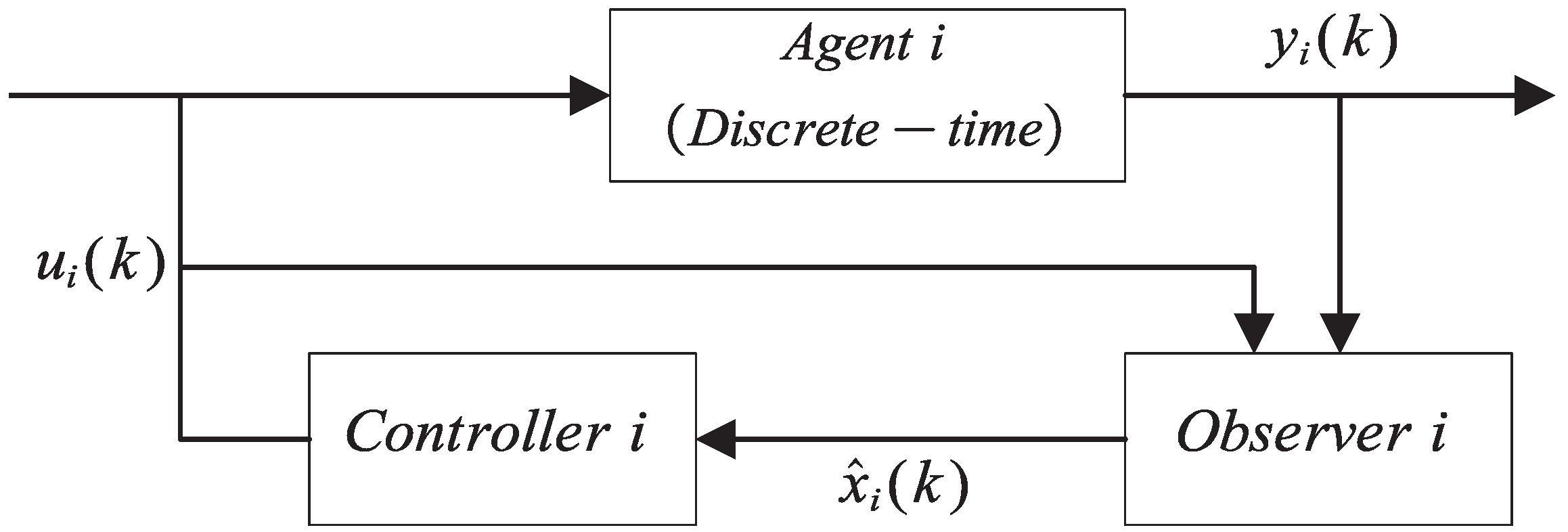
3.2. Observer-Based PID Protocol of Homogeneous PMASs

In this subsection, we construct an observer-based PID control protocol for the system (2). In [48], it has been verified that a positive system is not stabilized by using a Luenberger observer-based controller. Thus, it is not hard to derive that the system (2) is not stabilized by virtue of a dynamic control protocol with the observer (3). Following the design in [49], an improved observer is designed as:

$$\begin{array}{c}{\widehat{x}}_i(k+1)=E{\widehat{x}}_i\left(k\right)+L{y}_i\left(k\right),\hfill \end{array}$$

(8)

where $\widehat{x}\left(k\right)\in {\mathbb{R}}^s$ is the state of observer, $y_i\left(k\right)\in {\mathbb{R}}^q$ is the output of system (2), and $E\in {\mathbb{R}}^{s\times s}$ and $L\in {\mathbb{R}}^{s\times q}$ are the observer gain matrices to be determined. Based on the observer (8), a PID control protocol is constructed as:

$$\begin{array}{c}{u}_i\left(k\right)=K_S{\widehat{x}}_i\left(k\right)+K_P\sum _{j\in {\mathcal{N}}_i}{a}_{ij}({\widehat{x}}_i\left(k\right)-{\widehat{x}}_j\left(k\right))+K_I\sum _{h=k-d}^{k-1}{\widehat{x}}_i\left(h\right)+K_D\Delta {\widehat{x}}_i\left(k\right),\hfill \end{array}$$

(9)

where $K_S,K_P,K_I$, and $K_D$ are PID controller gain matrices to be designed, d is the time delay, and $\Delta {\widehat{x}}_i\left(k\right)={\widehat{x}}_i\left(k\right)-{\widehat{x}}_i(k-1)$. The estimate error is defined as: ${\tilde{e}}_i\left(k\right)=x_i\left(k\right)-{\widehat{x}}_i\left(k\right).$

Choose ${\tilde{x}}_i\left(k\right):={({\widehat{x}}_i^{\top }\left(k\right),{\tilde{e}}_i^{\top }\left(k\right))}^{\top }$ and ${\tilde{y}}_i\left(k\right):={\widehat{x}}_i\left(k\right)$ as the state variable and output, respectively. Then the augmented system of agent i with the observer-based PID control input (9) is:

$$\begin{array}{c}{\tilde{x}}_i(k+1)=\tilde{A}{\tilde{x}}_i\left(k\right)+\tilde{B}{u}_i\left(k\right),\hfill \\ {\tilde{y}}_i\left(k\right)=\tilde{C}{\tilde{x}}_i\left(k\right),\hfill \end{array}$$

(10)

where

$$\begin{array}{c}\tilde{A}=\left(\begin{array}{cc}E+LC& LC\\ A-LC-E& A-LC\end{array}\right),\tilde{B}=\left(\begin{array}{c}0\\ B\end{array}\right),\tilde{C}=\left(\begin{array}{cc}I& 0\end{array}\right).\hfill \end{array}$$

Let $\mathcal{X}\left(k\right)={({\tilde{x}}_1^{\top }\left(k\right),{\tilde{x}}_2^{\top }\left(k\right),\cdots ,{\tilde{x}}_n^{\top }\left(k\right))}^{\top }$. The overall closed-loop system can be written in a compact form as:

$$\begin{array}{c}\mathcal{X}(k+1)=\mathbb{A}\mathcal{X}\left(k\right)+{\mathbb{B}}_1\mathcal{X}(k-1)+\sum _{h=k-d}^{k-2}{\mathbb{B}}_2\mathcal{X}\left(h\right),\hfill \end{array}$$

(11)

where

$$\begin{array}{c}\mathbb{A}=I_n\otimes \check{A}+\mathcal{L}\otimes \tilde{B}{K}_P\tilde{C},\mathbb{B}=I_n\otimes \left(\tilde{B}(K_I-K_D)\tilde{C}\right),\\ \check{A}=\left(\begin{array}{cc}E+LC& LC\\ A+B{K}_S+B{K}_D-LC-E& A-LC\end{array}\right),\tilde{B}=\left(\begin{array}{c}0\\ B\end{array}\right),\tilde{C}=\left(\begin{array}{cc}I& 0\end{array}\right).\end{array}$$

(12)

Thus, the entries of matrices $\mathbb{A}$, ${\mathbb{B}}_1,$ and ${\mathbb{B}}_2$ can be shown as:

$$\begin{array}{c}{\mathbb{A}}_{ii}=\left(\begin{array}{cc}E+LC& LC\\ A-LC-E+\sum _{j\in {\mathcal{N}}_1}{a}_{ij}B{K}_P+B{K}_S+B{K}_D& A-LC\end{array}\right),\\ {\mathbb{A}}_{ij}=\left(\begin{array}{cc}0& 0\\ -a_{ij}B{K}_P& 0\end{array}\right),{\mathbb{B}}_{1_{ii}}=\left(\begin{array}{cc}0& 0\\ B{K}_I-B{K}_D& 0\end{array}\right),{\mathbb{B}}_{2_{ii}}=\left(\begin{array}{cc}0& 0\\ B{K}_I& 0\end{array}\right).\end{array}$$

(13)

Remark 2.

The observer (8) is different from the Luenberger observer in [50]. It can be observed from (10)–(13) that the observer gain matrices $E,$ and L and the controller gain matrices $K_S,K_P,K_I,$ and $K_D$ are independent. Therefore, the observer-based PID control in this paper cannot be designed separately. The consensus problem of positive discrete-time multi-agent system (2) with the observer-based PID control protocol (8) can be transformed into the consensus problem of the augmented system (11).

Theorem 2.

If there exist constants ${\lambda }_1>0,{\lambda }_2>1,{\mathbb{R}}^s$ vectors ${\varsigma }_1\succ 0,{\varsigma }_2\succ 0,{\zeta }_1\succ 0,{\zeta }_2\succ 0,{\xi }_1\succ 0,{\xi }_2\succ 0,{\underline{\delta }}_{ec}\succ 0,{\delta }_{ec}^{\left(ı\right)}\succ 0,{\overline{\delta }}_{ec}\succ 0,{\delta }_{ks}^{\left(𝒥\right)},{\delta }_{ks},{\delta }_{kp}^{\left(𝒥\right)}\prec 0,{\delta }_{kp}\prec 0,{\delta }_{ki}^{\left(𝒥\right)}\succ 0,{\delta }_{ki}\succ 0,{\underline{\delta }}_{kd},{\delta }_{kd}^{\left(𝒥\right)},{\delta }_{kd}$, and ${\mathbb{R}}^q$ vectors ${\underline{\delta }}_{lc}\succ 0,{\delta }_{lc}^{\left(ı\right)}\succ 0,{\overline{\delta }}_{lc}\succ 0$ such that

$$\begin{array}{c}{\lambda }_1{\mathbf{1}}_m^{\top }{B}^{\top }{\varsigma }_{2}A-\sum _{ı=1}^s{\mathbf{1}}_s^{\left(ı\right)}{\delta }_{ec}^{\left(ı\right)\top }-\sum _{ı=1}^s{\mathbf{1}}_s^{\left(ı\right)}{\delta }_{lc}^{\left(ı\right)\top }C+{\lambda }_{1}B\sum _{𝒥=1}^m{\mathbf{1}}_m^{\left(𝒥\right)}{\delta }_{ks}^{\left(𝒥\right)\top }\\ +{\lambda }_{1}B\sum _{𝒥=1}^m{\mathbf{1}}_m^{\left(𝒥\right)}{\delta }_{kd}^{\left(𝒥\right)\top }+{\lambda }_1\sum _{j\in {\mathcal{N}}_1}{a}_{1j}B\sum _{𝒥=1}^m{\mathbf{1}}_m^{\left(𝒥\right)}{\delta }_{kp}^{\left(𝒥\right)\top }⪰0,\end{array}$$

(14a)

$$\begin{array}{c}{\mathbf{1}}_s^{\top }{\varsigma }_{1}A-\sum _{ı=1}^s{\mathbf{1}}_s^{\left(ı\right)}{\delta }_{lc}^{\left(ı\right)\top }C⪰0,\end{array}$$

(14b)

$$\begin{array}{c}\sum _{𝒥=1}^m{\mathbf{1}}_m^{\left(𝒥\right)}{\delta }_{ki}^{\left(𝒥\right)\top }-\sum _{𝒥=1}^m{\mathbf{1}}_m^{\left(𝒥\right)}{\delta }_{kd}^{\left(𝒥\right)\top }⪰0,\end{array}$$

(14c)

$$\begin{array}{c}{\lambda }_1{\mathbf{1}}_m^{\top }{B}^{\top }{\varsigma }_2⪯{\mathbf{1}}_s^{\top }{\varsigma }_1,\end{array}$$

(14d)

$$\begin{array}{c}{\lambda }_2{\varsigma }_1⪯{\varsigma }_2,\end{array}$$

(14e)

$$\begin{array}{c}{\underline{\delta }}_{ec}⪯{\delta }_{ec}^{\left(ı\right)}⪯{\overline{\delta }}_{ec},{\underline{\delta }}_{lc}⪯{\delta }_{lc}^{\left(ı\right)}⪯{\overline{\delta }}_{lc},ı=1,2,\cdots ,s,\end{array}$$

(14f)

$$\begin{array}{c}{\delta }_{ks}^{\left(𝒥\right)}⪯{\delta }_{ks},{\delta }_{kp}^{\left(𝒥\right)}⪯{\delta }_{kp},{\delta }_{ki}^{\left(𝒥\right)}⪯{\delta }_{ki},{\underline{\delta }}_{kd}⪯{\delta }_{kd}^{\left(𝒥\right)}⪯{\overline{\delta }}_{kd},𝒥=1,2,\cdots ,m,\end{array}$$

(14g)

$$\begin{array}{c}{A}^{\top }{\varsigma }_2+(1-{\lambda }_2)C^{\top }{\underline{\delta }}_{lc}+(1-{\lambda }_2){\underline{\delta }}_{ec}+{\overline{\delta }}_{ks}+{\overline{\delta }}_{kd}+{\zeta }_1-{\varsigma }_1\prec 0,\end{array}$$

(14h)

$$\begin{array}{c}(A^{\top }-I){\varsigma }_2+(1-{\lambda }_2)C^{\top }{\underline{\delta }}_{lc}+{\zeta }_2\prec 0,\end{array}$$

(14i)

$$\begin{array}{c}{\delta }_{ki}-{\underline{\delta }}_{kd}-{\zeta }_1+(d-1){\xi }_1\prec 0,\end{array}$$

(14j)

$$\begin{array}{c}(d-1){\xi }_2-{\zeta }_2\prec 0,\end{array}$$

(14k)

$$\begin{array}{c}{\overline{\delta }}_{ki}-{\xi }_1\prec 0,\end{array}$$

(14l)

hold, then under the observer-based PID control protocol (9) with

$$\begin{array}{c}E=\frac{{\sum }_{ı=1}^s{\mathbf{1}}_s^{\left(ı\right)}{\delta }_{ec}^{\left(ı\right)\top }}{{\mathbf{1}}_s^{\top }{\varsigma }_1},L=\frac{{\sum }_{ı=1}^s{\mathbf{1}}_s^{\left(ı\right)}{\delta }_{lc}^{\left(ı\right)\top }}{{\mathbf{1}}_s^{\top }{\varsigma }_1},K_S=\frac{{\sum }_{𝒥=1}^m{\mathbf{1}}_m^{\left(𝒥\right)}{\delta }_{ks}^{\left(𝒥\right)\top }}{{\mathbf{1}}_m^{\top }{B}^{\top }{\varsigma }_2},\\ K_P=\frac{{\sum }_{𝒥=1}^m{\mathbf{1}}_m^{\left(𝒥\right)}{\delta }_{kp}^{\left(𝒥\right)\top }}{{\mathbf{1}}_m^{\top }{B}^{\top }{\varsigma }_2},K_I=\frac{{\sum }_{𝒥=1}^m{\mathbf{1}}_m^{\left(𝒥\right)}{\delta }_{ki}^{\left(𝒥\right)\top }}{{\mathbf{1}}_m^{\top }{B}^{\top }{\varsigma }_2},K_D=\frac{{\sum }_{𝒥=1}^m{\mathbf{1}}_m^{\left(𝒥\right)}{\delta }_{kd}^{\left(𝒥\right)\top }}{{\mathbf{1}}_m^{\top }{B}^{\top }{\varsigma }_2},\end{array}$$

(15)

the closed-loop system (11) is positive and stable, which means that the observer (8) is positive and the consensus of system (2) is reached.

Proof of Theorem 2.

First, we prove the positivity of the closed-loop system (11). From (14a) and (14d), it can be obtained that

$$\begin{array}{cc}\hfill & A-\frac{{\sum }_{ı=1}^s{\mathbf{1}}_s^{\left(ı\right)}{\delta }_{ec}^{\left(ı\right)\top }}{{\mathbf{1}}_s^{\top }{\varsigma }_1}-\frac{{\sum }_{ı=1}^s{\mathbf{1}}_s^{\left(ı\right)}{\delta }_{lc}^{\left(ı\right)\top }}{{\mathbf{1}}_s^{\top }{\varsigma }_1}C+B\frac{{\sum }_{𝒥=1}^m{\mathbf{1}}_m^{\left(𝒥\right)}{\delta }_{ks}^{\left(𝒥\right)\top }}{{\mathbf{1}}_m^{\top }{B}^{\top }{\varsigma }_2}+B\frac{{\sum }_{𝒥=1}^m{\mathbf{1}}_m^{\left(𝒥\right)}{\delta }_{kd}^{\left(𝒥\right)\top }}{{\mathbf{1}}_m^{\top }{B}^{\top }{\varsigma }_2}+\sum _{j\in {\mathcal{N}}_1}{a}_{1j}B\frac{{\sum }_{𝒥=1}^m{\mathbf{1}}_m^{\left(𝒥\right)}{\delta }_{kp}^{\left(𝒥\right)\top }}{{\mathbf{1}}_m^{\top }{B}^{\top }{\varsigma }_2}\hfill \\ \hfill & ⪰A-\frac{{\sum }_{ı=1}^s{\mathbf{1}}_s^{\left(ı\right)}{\delta }_{ec}^{\left(ı\right)\top }}{{\lambda }_1{\mathbf{1}}_m^{\top }{B}^{\top }{\varsigma }_2}-\frac{{\sum }_{ı=1}^s{\mathbf{1}}_s^{\left(ı\right)}{\delta }_{lc}^{\left(ı\right)\top }}{{\lambda }_1{\mathbf{1}}_m^{\top }{B}^{\top }{\varsigma }_2}C+B\frac{{\sum }_{𝒥=1}^m{\mathbf{1}}_m^{\left(𝒥\right)}{\delta }_{ks}^{\left(𝒥\right)\top }}{{\mathbf{1}}_m^{\top }{B}^{\top }{\varsigma }_2}+B\frac{{\sum }_{𝒥=1}^m{\mathbf{1}}_m^{\left(𝒥\right)}{\delta }_{kd}^{\left(𝒥\right)\top }}{{\mathbf{1}}_m^{\top }{B}^{\top }{\varsigma }_2}+\sum _{j\in {\mathcal{N}}_1}{a}_{1j}B\frac{{\sum }_{𝒥=1}^m{\mathbf{1}}_m^{\left(𝒥\right)}{\delta }_{kp}^{\left(𝒥\right)\top }}{{\mathbf{1}}_m^{\top }{B}^{\top }{\varsigma }_2}⪰0.\hfill \end{array}$$

Together with (15), it is easy to derived that $A-LC-E+{\sum }_{j\in {\mathcal{N}}_1}{a}_{ij}B{K}_P+B{K}_S+B{K}_D⪰0$. Similarly, $A-LC⪰0$ can be obtained by (14b) and (15). Since ${\delta }_{ec}⪰0$ and ${\delta }_{lc}⪰0$, one has $E+LC⪰0$ and $LC⪰0$. Consequently, it follows that ${\mathbb{A}}_{ii}⪰0$. By $a_{ij}\ge 0$ and ${\delta }_{kp}^{\left(ı\right)}⪯0$, we have $-a_{ij}B{K}_P⪰0$. It means that ${\mathbb{A}}_{ij}⪰0$. Then it can be obtained that $\mathbb{A}⪰0$. Using (14c) and (15) gives $B{K}_I-B{K}_D⪰0$ and $B{K}_I⪰0$. Thus, ${\mathbb{B}}_1⪰0$ and ${\mathbb{B}}_2⪰0$. Therefore, the positivity of the overall closed-loop system (11) can be guaranteed by Lemma 1.

Next, we analyze the stability of the closed-loop system (11). Select the following copositive Lyapunov–Krasovskii function:

$$\begin{array}{c}V\left(k\right)={\mathcal{X}}^{\top }\left(k\right)v+{\mathcal{X}}^{\top }(k-1)\mu +\sum _{l=2}^d\sum _{h=k-l}^{k-2}{\mathcal{X}}^{\top }\left(h\right)\vartheta ,\end{array}$$

(16)

where $v={(\underset{n}{\underbrace{{\varsigma }^{\top },{\varsigma }^{\top },\cdots ,{\varsigma }^{\top }}})}^{\top }$, $\mu ={(\underset{n}{\underbrace{{\zeta }^{\top },{\zeta }^{\top },\cdots ,{\zeta }^{\top }}})}^{\top }$, $\vartheta =(\underset{n}{\underbrace{{\xi }^{\top },{\xi }^{\top },\cdots ,{\xi }^{\top }}})$, with $\varsigma ={({\varsigma }_1^{\top },{\varsigma }_2^{\top })}^{\top },\zeta ={({\zeta }_1^{\top },{\zeta }_2^{\top })}^{\top },\xi ={({\xi }_1^{\top },{\xi }_2^{\top })}^{\top }$, respectively. The derivative of $V\left(k\right)$ can be obtained as:

$$\begin{array}{cc}\Delta V\left(k\right)\hfill & =V(k+1)-V\left(k\right)\hfill \\ \hfill & ={\mathcal{X}}^{\top }(k+1)v+{\mathcal{X}}^{\top }\left(k\right)\mu +\sum _{l=2}^d\sum _{h=k-l+1}^{k-1}{\mathcal{X}}^{\top }\left(h\right)\vartheta -{\mathcal{X}}^{\top }\left(k\right)v\hfill \\ \hfill & -{\mathcal{X}}^{\top }(k-1)\mu -\sum _{l=2}^d\sum _{h=k-l}^{k-2}{\mathcal{X}}^{\top }\left(h\right)\vartheta \hfill \\ \hfill & ={\mathcal{X}}^{\top }\left(k\right){\mathbb{A}}^{\top }v+{\mathcal{X}}^{\top }(k-1){\mathbb{B}}_1^{\top }v+\sum _{h=k-d}^{k-2}{\mathcal{X}}^{\top }\left(h\right){\mathbb{B}}_2^{\top }v\hfill \\ \hfill & +{\mathcal{X}}^{\top }\left(k\right)\mu +\sum _{l=2}^d\sum _{h=k-l+1}^{k-1}{\mathcal{X}}^{\top }\left(h\right)\vartheta -{\mathcal{X}}^{\top }\left(k\right)v\hfill \\ \hfill & -{\mathcal{X}}^{\top }(k-1)\mu -\sum _{l=2}^d\sum _{h=k-l}^{k-2}{\mathcal{X}}^{\top }\left(h\right)\vartheta {\mathcal{X}}^{\top }\left(k\right)\hfill \\ \hfill & ={\mathcal{X}}^{\top }\left(k\right)({\mathbb{A}}^{\top }v+\mu -v)+{\mathcal{X}}^{\top }(k-1)({\mathbb{B}}_1^{\top }v-\mu +(d-1)\vartheta )\hfill \\ \hfill & +\sum _{h=k-d}^{k-2}{\mathcal{X}}^{\top }\left(h\right)({\mathbb{B}}_2^{\top }v-\vartheta ),\hfill \end{array}$$

(17)

combined with (13), we have

$$\begin{array}{cc}\hfill & {\mathbb{A}}^{\top }v+\mu -v\hfill \\ \hfill & ={\left(\begin{array}{ccccccc}E+LC& LC& 0& 0& \cdots & 0& 0\\ \mathsf{\Psi }& A-LC& -a_{12}B{K}_P& 0& \cdots & -a_{1n}B{K}_P& 0\\ 0& 0& E+LC& LC& \cdots & 0& 0\\ -a_{21}B{K}_P& 0& \mathsf{\Psi }& A-LC& \cdots & -a_{2n}B{K}_P& 0\\ ⋮& ⋮& ⋮& ⋮& \ddots & ⋮& ⋮\\ 0& 0& 0& 0& \cdots & E+LC& LC\\ -a_{n1}B{K}_P& 0& -a_{n2}B{K}_P& 0& \cdots & \mathsf{\Psi }& A-LC\end{array}\right)}^{\top }\left(\begin{array}{c}{\varsigma }_1\\ {\varsigma }_2\\ {\varsigma }_1\\ {\varsigma }_2\\ ⋮\\ {\varsigma }_1\\ {\varsigma }_2\end{array}\right)+\left(\begin{array}{c}{\zeta }_1\\ {\zeta }_2\\ {\zeta }_1\\ {\zeta }_2\\ ⋮\\ {\zeta }_1\\ {\zeta }_2\end{array}\right)-\left(\begin{array}{c}{\varsigma }_1\\ {\varsigma }_2\\ {\varsigma }_1\\ {\varsigma }_2\\ ⋮\\ {\varsigma }_1\\ {\varsigma }_2\end{array}\right)\hfill \\ \hfill & =\left(\begin{array}{c}{E}^{\top }{\varsigma }_1+C^{\top }{L}^{\top }{\varsigma }_1+A^{\top }{\varsigma }_2-C^{\top }{L}^{\top }{\varsigma }_2-E^{\top }{\varsigma }_2+K_S^{\top }{B}^{\top }{\varsigma }_2+K_D^{\top }{B}^{\top }{\varsigma }_2+\Theta +{\zeta }_1-{\varsigma }_1\\ C^{\top }{L}^{\top }{\varsigma }_1+A^{\top }{\varsigma }_2-C^{\top }{L}^{\top }{\varsigma }_2+{\zeta }_2-{\varsigma }_2\\ E^{\top }{\varsigma }_1+C^{\top }{L}^{\top }{\varsigma }_1+A^{\top }{\varsigma }_2-C^{\top }{L}^{\top }{\varsigma }_2-E^{\top }{\varsigma }_2+K_S^{\top }{B}^{\top }{\varsigma }_2+K_D^{\top }{B}^{\top }{\varsigma }_2+\Theta +{\zeta }_1-{\varsigma }_1\\ C^{\top }{L}^{\top }{\varsigma }_1+A^{\top }{\varsigma }_2-C^{\top }{L}^{\top }{\varsigma }_2+{\zeta }_2-{\varsigma }_2\\ ⋮\\ E^{\top }{\varsigma }_1+C^{\top }{L}^{\top }{\varsigma }_1+A^{\top }{\varsigma }_2-C^{\top }{L}^{\top }{\varsigma }_2-E^{\top }{\varsigma }_2+K_S^{\top }{B}^{\top }{\varsigma }_2+K_D^{\top }{B}^{\top }{\varsigma }_2+\Theta +{\zeta }_1-{\varsigma }_1\\ C^{\top }{L}^{\top }{\varsigma }_1+A^{\top }{\varsigma }_2-C^{\top }{L}^{\top }{\varsigma }_2+{\zeta }_2-{\varsigma }_2\end{array}\right),\hfill \end{array}$$

(18)

$$\begin{array}{cc}\hfill & {\mathbb{B}}^{\top }v-\mu +(d-1)\vartheta \hfill \\ \hfill & =\left(\begin{array}{c}{\left(\begin{array}{cc}0& 0\\ B{K}_I-B{K}_D& 0\end{array}\right)}^{\top }\left(\begin{array}{c}{\varsigma }_1\\ {\varsigma }_2\end{array}\right)-\left(\begin{array}{c}{\zeta }_1\\ {\zeta }_2\end{array}\right)+(d-1)\left(\begin{array}{c}{\xi }_1\\ {\xi }_2\end{array}\right)\\ {\left(\begin{array}{cc}0& 0\\ B{K}_I-B{K}_D& 0\end{array}\right)}^{\top }\left(\begin{array}{c}{\varsigma }_1\\ {\varsigma }_2\end{array}\right)-\left(\begin{array}{c}{\zeta }_1\\ {\zeta }_2\end{array}\right)+(d-1)\left(\begin{array}{c}{\xi }_1\\ {\xi }_2\end{array}\right)\\ ⋮\\ {\left(\begin{array}{cc}0& 0\\ B{K}_I-B{K}_D& 0\end{array}\right)}^{\top }\left(\begin{array}{c}{\varsigma }_1\\ {\varsigma }_2\end{array}\right)-\left(\begin{array}{c}{\zeta }_1\\ {\zeta }_2\end{array}\right)+(d-1)\left(\begin{array}{c}{\xi }_1\\ {\xi }_2\end{array}\right)\end{array}\right)=\left(\begin{array}{c}{K}_I^{\top }{B}^{\top }{\varsigma }_2-K_D^{\top }{B}^{\top }{\varsigma }_2-{\zeta }_1+(d-1){\xi }_1\\ (d-1){\xi }_2-{\zeta }_2\\ K_I^{\top }{B}^{\top }{\varsigma }_2-K_D^{\top }{B}^{\top }{\varsigma }_2-{\zeta }_1+(d-1){\xi }_1\\ (d-1){\xi }_2-{\zeta }_2\\ ⋮\\ K_I^{\top }{B}^{\top }{\varsigma }_2-K_D^{\top }{B}^{\top }{\varsigma }_2-{\zeta }_1+(d-1){\xi }_1\\ (d-1){\xi }_2-{\zeta }_2\end{array}\right),\hfill \end{array}$$

(19)

and

$$\begin{array}{c}{\mathbb{B}}_{2}v-\vartheta ={\left(\begin{array}{ccccccc}0& 0& 0& 0& \cdots & 0& 0\\ B{K}_I& 0& 0& 0& \cdots & 0& 0\\ 0& 0& 0& 0& \cdots & 0& 0\\ 0& 0& B{K}_I& 0& \cdots & 0& 0\\ ⋮& ⋮& ⋮& ⋮& \ddots & ⋮& ⋮\\ 0& 0& 0& 0& \cdots & 0& 0\\ 0& 0& 0& 0& \cdots & B{K}_I& 0\end{array}\right)}^{\top }\left(\begin{array}{c}{\varsigma }_1\\ {\varsigma }_2\\ {\varsigma }_1\\ {\varsigma }_2\\ ⋮\\ {\varsigma }_1\\ {\varsigma }_2\end{array}\right)-\left(\begin{array}{c}{\xi }_1\\ {\xi }_2\\ {\xi }_1\\ {\xi }_2\\ ⋮\\ {\xi }_1\\ {\xi }_2\end{array}\right)=\left(\begin{array}{c}{K}_I^{\top }{B}^{\top }{\varsigma }_2-{\xi }_1\\ -{\xi }_2\\ K_I^{\top }{B}^{\top }{\varsigma }_2-{\xi }_1\\ -{\xi }_2\\ ⋮\\ K_I^{\top }{B}^{\top }{\varsigma }_2-{\xi }_1\\ -{\xi }_2\end{array}\right),\hfill \end{array}$$

(20)

where $\mathsf{\Psi }=A-LC-E+{\sum }_{j\in {\mathcal{N}}_1}{a}_{1j}B{K}_P+B{K}_D$, $\Theta ={\sum }_{j\in {\mathcal{N}}_1}{a}_{1j}{K}_P^{\top }{B}^{\top }{\varsigma }_2-{\sum }_{j\in {\mathcal{N}}_1}{a}_{j1}{K}_P^{\top }{B}^{\top }{\varsigma }_2$. Owing to the symmetry of undirected topological graph, it can be obtained that $\Theta ={\sum }_{j\in {\mathcal{N}}_1}{a}_{1j}{K}_P^{\top }{B}^{\top }{\varsigma }_2-{\sum }_{j\in {\mathcal{N}}_1}{a}_{j1}{K}_P^{\top }{B}^{\top }{\varsigma }_2=0.$ By (14d)–(14g) and (15), it follows that

$$\begin{array}{c}{E}^{\top }({\varsigma }_1-{\varsigma }_2)=\frac{{\sum }_{ı=1}^s{\mathbf{1}}_s^{\left(ı\right)}{\delta }_{ec}^{\left(ı\right)\top }}{{\mathbf{1}}_s^{\top }{\varsigma }_1}({\varsigma }_1-{\varsigma }_2)⪯\frac{{\underline{\delta }}_{ec}{\mathbf{1}}_s^{\top }}{{\mathbf{1}}_s^{\top }{\varsigma }_1}({\varsigma }_1-{\lambda }_2{\varsigma }_1)=(1-{\lambda }_2){\underline{\delta }}_{ec},\\ L^{\top }({\varsigma }_1-{\varsigma }_2)=\frac{{\sum }_{ı=1}^s{\mathbf{1}}_s^{\left(ı\right)}{\delta }_{lc}^{\left(ı\right)\top }}{{\mathbf{1}}_s^{\top }{\varsigma }_1}({\varsigma }_1-{\varsigma }_2)⪯\frac{{\underline{\delta }}_{lc}{\mathbf{1}}_s^{\top }}{{\mathbf{1}}_s^{\top }{\varsigma }_1}({\varsigma }_1-{\lambda }_2{\varsigma }_1)=(1-{\lambda }_2){\underline{\delta }}_{lc},\\ {\underline{\delta }}_{kd}=\frac{{\underline{\delta }}_{kd}{\mathbf{1}}_m^{\top }}{{\mathbf{1}}_m^{\top }{B}^{\top }{\varsigma }_2}{B}^{\top }{\varsigma }_2⪯K_D^{\top }{B}^{\top }{\varsigma }_2=\frac{{\left({\sum }_{𝒥=1}^m{\mathbf{1}}_m^{\left(𝒥\right)}{\delta }_{kd}^{\left(𝒥\right)\top }\right)}^{\top }}{{\mathbf{1}}_m^{\top }{B}^{\top }{\varsigma }_2}{B}^{\top }{\varsigma }_2⪯\frac{{\overline{\delta }}_{kd}{\mathbf{1}}_m^{\top }}{{\mathbf{1}}_m^{\top }{B}^{\top }{\varsigma }_2}{B}^{\top }{\varsigma }_2={\overline{\delta }}_{kd},\\ K_I^{\top }{B}^{\top }{\varsigma }_2=\frac{{\left({\sum }_{𝒥=1}^m{\mathbf{1}}_m^{\left(𝒥\right)}{\delta }_{ki}^{\left(𝒥\right)\top }\right)}^{\top }}{{\mathbf{1}}_m^{\top }{B}^{\top }{\varsigma }_2}{B}^{\top }{\varsigma }_2⪯{\delta }_{ki},\\ K_S^{\top }{B}^{\top }{\varsigma }_2=\frac{{\left({\sum }_{𝒥=1}^m{\mathbf{1}}_m^{\left(𝒥\right)}{\delta }_{ks}^{\left(𝒥\right)\top }\right)}^{\top }}{{\mathbf{1}}_m^{\top }{B}^{\top }{\varsigma }_2}{B}^{\top }{\varsigma }_2⪯{\delta }_{ks}.\end{array}$$

(21)

Together (14h) with (18), and (21), it can be derived that

$$\begin{array}{cc}\hfill & E^{\top }{\varsigma }_1+C^{\top }{L}^{\top }{\varsigma }_1+A^{\top }{\varsigma }_2-E^{\top }{\varsigma }_2-C^{\top }{L}^{\top }{\varsigma }_2+K_S^{\top }{B}^{\top }{\varsigma }_2+K_D^{\top }{B}^{\top }{\varsigma }_2+{\zeta }_1-{\varsigma }_1\hfill \\ \hfill & =E^{\top }({\varsigma }_1-{\varsigma }_2)+C^{\top }{L}^{\top }({\varsigma }_1-{\varsigma }_2)+A^{\top }{\varsigma }_2+K_S^{\top }{B}^{\top }{\varsigma }_2+K_D^{\top }{B}^{\top }{\varsigma }_2+{\zeta }_1-{\varsigma }_1\hfill \\ \hfill & ⪯A^{\top }{\varsigma }_2+(1-{\lambda }_2)C^{\top }{\underline{\delta }}_{lc}+(1-{\lambda }_2){\underline{\delta }}_{ec}+{\overline{\delta }}_{ks}+{\overline{\delta }}_{kd}+{\zeta }_1-{\varsigma }_1\prec 0.\hfill \end{array}$$

(22)

Combining (14i), (18), and (21), we have

$$\begin{array}{c}{C}^{\top }{L}^{\top }{\varsigma }_1+A^{\top }{\varsigma }_2-C^{\top }{L}^{\top }{\varsigma }_2+{\zeta }_2-{\varsigma }_2⪯(A^{\top }-I){\varsigma }_2+(1-{\lambda }_2)C^{\top }{\underline{\delta }}_{lc}+{\zeta }_2⪯0.\end{array}$$

(23)

Using (14j), (14l), and(19)–(21), it gives that

$$\begin{array}{c}{K}_I^{\top }{B}^{\top }{\varsigma }_2-K_D^{\top }{B}^{\top }{\varsigma }_2-{\zeta }_1+(d-1){\xi }_1⪯{\delta }_{ki}-{\underline{\delta }}_{kd}-{\zeta }_1+(d-1){\xi }_1\prec 0,\end{array}$$

(24)

$$\begin{array}{c}{K}_I^{\top }{B}^{\top }{\varsigma }_2-{\xi }_1⪯{\overline{\delta }}_{ki}-{\xi }_1\prec 0.\end{array}$$

(25)

From (14k) and (22)–(25), it is easy to obtain that

$$\begin{array}{c}{\mathbb{A}}^{\top }v+\mu -v\prec 0,\\ {\mathbb{B}}_1^{\top }v-\mu +(d-1)\vartheta \prec 0,\\ {\mathbb{B}}_2^{\top }v-\vartheta \prec 0.\end{array}$$

which means that $\Delta V\left(k\right)<0$. □

Remark 3.

In the literature [39,41,42,43,44,45], the Luenberger-type observer-based protocols were employed for MASs. The designed observer (3) in our work is different from existing observers. Two gain matrices E and L are introduced in this paper. A matrix decomposition approach is employed to design the two matrices. This new observer can handle the consensus protocol issues of PMASs and thus the problem addressed in [48] can be solved. Moreover, the introduction of two gain matrices increases the degree of freedom of the observer design.

Remark 4.

The consensus problem of PMASs has been investigated from different perspectives. Existing works on the consensus of PMASs were developed in the form of proportional controllers [43,44,45,51,52,53,54,55]. As is well known, PID control offers higher stability performance in comparison to the proportional control. Theorem 2 designs a PID control protocol for PMASs. It can be seen that the PID controller (9) is completely different from these forms in [43,44,45,51,52,53,54,55]. Four control gain matrices $K_S,K_P,K_I,K_D$ need to be determined. The designed controller (9) takes four types of information: the estimated states of the agent itself, neighboring agents, time-delay information of the agent with length of d, and the differential information of the agent. It is clear that the existing protocol designs are special cases of (9) and the PID protocol in this paper has more degree of freedom in designing control gains.

Remark 5.

There is a significant difference between the designed observer-based PID control protocol of PMASs in this paper and the PID control protocol of general MASs in [56,57]. A quadratic approach is employed for general MASs while a linear approach is utilized for PMASs in this paper. Considering the positivity of PMASs, it is a natural choice to build a copositive Lyapunov–Krasovskii function and apply a linear computation method. Meanwhile, the designed Lyapunov–Krasovskii function has a simple form and linear programming is more effective in handling complex computations. It can be seen that all the conditions given in Theorem 2 are solvable in terms of linear programming. The conditions (14a)–(14d) guarantee the positivity of the overall closed-loop system (11). The difference (17) of the Lyapunov–Krasovskii function (16) is kept negative under the conditions of (14e)–(14l). Once the conditions in Theorem 2 have feasible solutions, the positivity and stability of the closed-loop system (11) can be guaranteed, which indicates that the consensus of system (2) is reached.

As mentioned in Remark 4, many existing protocol designs are special cases of (9) by using part of its components. It is similar to the hierarchical control designed in [52]. An observer-based hierarchical control protocol can be given as:

$$\begin{array}{c}{u}_i\left(k\right)=K_S{\widehat{x}}_i\left(k\right)+K_P\sum _{j\in {\mathcal{N}}_i}{a}_{ij}({\widehat{x}}_i\left(k\right)-{\widehat{x}}_j\left(k\right)),\hfill \end{array}$$

(26)

where $K_S{\widehat{x}}_i\left(k\right)$ and $K_P{\sum }_{j\in {\mathcal{N}}_i}{a}_{ij}({\widehat{x}}_i\left(k\right)-{\widehat{x}}_j\left(k\right))$ can be viewed as lower level and higher level contro protocol, respectively. $K_S$ and $K_P$ are the gain matrices need to determined. Similar to (11), the overall closed-loop system under the hierarchical protocol (26) is:

$$\begin{array}{c}\mathcal{X}(k+1)=\mathsf{A}\mathcal{X}\left(k\right),\hfill \end{array}$$

(27)

where

$$\begin{array}{c}\mathsf{A}=I_n\otimes \left(\begin{array}{cc}E+LC& LC\\ A+B{K}_S-LC-E& A-LC\end{array}\right)+\mathcal{L}\otimes \left(\begin{array}{cc}0& 0\\ B{K}_P& 0\end{array}\right).\hfill \end{array}$$

Corollary 1.

If there exist constants ${\lambda }_1>0,{\lambda }_2>1,{\mathbb{R}}^s$ vectors ${\varsigma }_1\succ 0,{\varsigma }_2\succ 0,{\underline{\delta }}_{ec}\succ 0,{\delta }_{ec}^{\left(ı\right)}\succ 0,{\overline{\delta }}_{ec}\succ 0,{\delta }_{ks}^{\left(𝒥\right)},{\delta }_{ks},{\delta }_{kp}^{\left(𝒥\right)}\prec 0,{\delta }_{kp}\prec 0,$ and ${\mathbb{R}}^q$ vectors ${\underline{\delta }}_{lc}\succ 0,{\delta }_{lc}^{\left(ı\right)}\succ 0,{\overline{\delta }}_{lc}\succ 0$ such that

$$\begin{array}{c}{\lambda }_1{\mathbf{1}}_m^{\top }{B}^{\top }{\varsigma }_{2}A-\sum _{ı=1}^s{\mathbf{1}}_s^{\left(ı\right)}{\delta }_{ec}^{\left(ı\right)\top }-\sum _{ı=1}^s{\mathbf{1}}_s^{\left(ı\right)}{\delta }_{lc}^{\left(ı\right)\top }C\\ +{\lambda }_{1}B\sum _{𝒥=1}^m{\mathbf{1}}_m^{\left(𝒥\right)}{\delta }_{ks}^{\left(𝒥\right)\top }+{\lambda }_1\sum _{j\in {\mathcal{N}}_1}{a}_{1j}B\sum _{𝒥=1}^m{\mathbf{1}}_m^{\left(𝒥\right)}{\delta }_{kp}^{\left(𝒥\right)\top }⪰0,\end{array}$$

$$\begin{array}{c}{\mathbf{1}}_s^{\top }{\varsigma }_{1}A-\sum _{ı=1}^s{\mathbf{1}}_s^{\left(ı\right)}{\delta }_{lc}^{\left(ı\right)\top }C⪰0,\end{array}$$

$$\begin{array}{c}{\lambda }_1{\mathbf{1}}_m^{\top }{B}^{\top }{\varsigma }_2⪯{\mathbf{1}}_s^{\top }{\varsigma }_1,\end{array}$$

$$\begin{array}{c}{\lambda }_2{\varsigma }_1⪯{\varsigma }_2,\end{array}$$

$$\begin{array}{c}{\underline{\delta }}_{ec}⪯{\delta }_{ec}^{\left(ı\right)}⪯{\overline{\delta }}_{ec},{\underline{\delta }}_{lc}⪯{\delta }_{lc}^{\left(ı\right)}⪯{\overline{\delta }}_{lc},ı=1,2,\cdots ,s,\end{array}$$

$$\begin{array}{c}{\delta }_{ks}^{\left(𝒥\right)}⪯{\delta }_{ks},{\delta }_{kp}^{\left(𝒥\right)}⪯{\delta }_{kp},𝒥=1,2,\cdots ,m,\end{array}$$

$$\begin{array}{c}{A}^{\top }{\varsigma }_2+(1-{\lambda }_2)C^{\top }{\underline{\delta }}_{lc}+(1-{\lambda }_2){\underline{\delta }}_{ec}+{\overline{\delta }}_{ks}-{\varsigma }_1\prec 0,\end{array}$$

$$\begin{array}{c}(A^{\top }-I){\varsigma }_2+(1-{\lambda }_2)C^{\top }{\underline{\delta }}_{lc}\prec 0,\end{array}$$

hold, then under the observer-based hierarchical control protocol (26) with

$$\begin{array}{c}E=\frac{{\sum }_{ı=1}^s{\mathbf{1}}_s^{\left(ı\right)}{\delta }_{ec}^{\left(ı\right)\top }}{{\mathbf{1}}_s^{\top }{\varsigma }_1},L=\frac{{\sum }_{ı=1}^s{\mathbf{1}}_s^{\left(ı\right)}{\delta }_{lc}^{\left(ı\right)\top }}{{\mathbf{1}}_s^{\top }{\varsigma }_1},K_S=\frac{{\sum }_{𝒥=1}^m{\mathbf{1}}_m^{\left(𝒥\right)}{\delta }_{ks}^{\left(𝒥\right)\top }}{{\mathbf{1}}_m^{\top }{B}^{\top }{\varsigma }_2},K_P=\frac{{\sum }_{𝒥=1}^m{\mathbf{1}}_m^{\left(𝒥\right)}{\delta }_{kp}^{\left(𝒥\right)\top }}{{\mathbf{1}}_m^{\top }{B}^{\top }{\varsigma }_2},\end{array}$$

the closed-loop system (27) is positive and stable, which means that the observer (8) is positive and the consensus of system (2) is reached.

Proof of Corollary 1.

The proof of Corollary 1 is similar to Theorem 2 and thus omitted. □

3.3. Observer-Based PID Control for Heterogeneous PMASs

Theorems 1 and 2 assume that each agent is homogeneous, that is, each agent has the same system dynamics. However, in practice systems, each agent may have different system dynamics. This kind of PMASs can be described as follows:

$$\begin{array}{c}{x}_{\iota }(k+1)=A_{\iota }{x}_{\iota }\left(k\right)+B_{\iota }{u}_{\iota }\left(k\right),\hfill \\ y_{\iota }\left(k\right)=C_{\iota }{x}_{\iota }\left(k\right),\iota \in \mathcal{V},\hfill \end{array}$$

(28)

where $A_{\iota }\in {\mathbb{R}}^{s\times s},B_{\iota }\in {\mathbb{R}}^{s\times m},C_{\iota }\in {\mathbb{R}}^{s\times q}$ are the system matrices of the $\iota$th agent. Furthermore, the observer of $\iota$th agent can be constructed as:

$$\begin{array}{c}{\widehat{x}}_{\iota }(k+1)=E_{\iota }{\widehat{x}}_{\iota }\left(k\right)+L_{\iota }{y}_{\iota }\left(k\right),\hfill \end{array}$$

(29)

where $E_{\iota }\in {\mathbb{R}}^{s\times s}$ and $L_{\iota }\in {\mathbb{R}}^{s\times q}$ are gain matrices to be determined. The estimate error is described as: ${\tilde{e}}_{\iota }\left(k\right)=x_{\iota }\left(k\right)-{\widehat{x}}_{\iota }\left(k\right)$. The corresponding observer-based PID control protocol for the $\iota$th agent is given by:

$$\begin{array}{c}{u}_{\iota }\left(k\right)=K_{S_{\iota }}{\widehat{x}}_{\iota }\left(k\right)+K_{P_{\iota }}\sum _{j\in {\mathcal{N}}_{\iota }}{a}_{\iota j}({\widehat{x}}_{\iota }\left(k\right)-{\widehat{x}}_j\left(k\right))+K_{I_{\iota }}\sum _{h=k-d}^{k-1}{\widehat{x}}_{\iota }\left(h\right)+K_{D_{\iota }}\Delta {\widehat{x}}_{\iota }\left(k\right),\hfill \end{array}$$

(30)

where $K_{S_{\iota }},K_{P_{\iota }},K_{I_{\iota }}$, and $K_{D_{\iota }}$ are control gain matrices to be determined.

Define ${\tilde{x}}_{\iota }(k+1)={({\widehat{x}}_{\iota }^{\top }(k+1),{\tilde{e}}_{\iota }^{\top }(k+1))}^{\top }$, the augmented system of the $\iota$th agent can be described as:

$$\begin{array}{cc}\hfill & {\tilde{x}}_{\iota }(k+1)={\tilde{A}}_{\iota }{\tilde{x}}_{\iota }\left(k\right)+{\tilde{B}}_{\iota }{u}_{\iota }\left(k\right),\hfill \\ \hfill & {\tilde{y}}_{\iota }\left(k\right)=\tilde{C}{\tilde{x}}_{\iota }\left(k\right),\hfill \end{array}$$

(31)

where

$$\begin{array}{c}{\tilde{A}}_{\iota }=\left(\begin{array}{cc}{E}_{\iota }+L_{\iota }{C}_{\iota }& L_{\iota }{C}_{\iota }\\ A_{\iota }-L_{\iota }{C}_{\iota }-E_{\iota }& A_{\iota }-L_{\iota }{C}_{\iota }\end{array}\right),{\tilde{B}}_{\iota }=\left(\begin{array}{c}0\\ B_{\iota }\end{array}\right),\tilde{C}=\left(\begin{array}{cc}I& 0\end{array}\right).\end{array}$$

The overall closed-loop system under the controller (30) is expressed as:

$$\begin{array}{c}\mathcal{X}(k+1)=\mathbb{A}\mathcal{X}\left(k\right)+{\mathbb{B}}_1\mathcal{X}(k-1)+\sum _{h=k-d}^{k-2}{\mathbb{B}}_2\mathcal{X}\left(h\right),\end{array}$$

(32)

where

$$\begin{array}{c}{\mathbb{A}}_{\iota \iota }=\left(\begin{array}{cc}{E}_{\iota }+L_{\iota }{C}_{\iota }& L_{\iota }{C}_{\iota }\\ A_{\iota }-L_{\iota }{C}_{\iota }-E_{\iota }+\sum _{j\in {\mathcal{N}}_{\iota }}{a}_{\iota j}{B}_{\iota }{K}_{P_{\iota }}+B_{\iota }{K}_{S_{\iota }}+B_{\iota }{K}_{D_{\iota }}& A_{\iota }-L_{\iota }{C}_{\iota }\end{array}\right),\hfill \\ {\mathbb{A}}_{ıj}=\left(\begin{array}{cc}0& 0\\ -a_{ıj}B{K}_{P_{\iota }}& 0\end{array}\right),{\mathbb{B}}_{1_{\iota \iota }}=\left(\begin{array}{cc}0& 0\\ B_{\iota }{K}_{I_{\iota }}-B_{\iota }{K}_{D_{\iota }}& 0\end{array}\right),{\mathbb{B}}_{2_{\iota \iota }}=\left(\begin{array}{cc}0& 0\\ B_{\iota }{K}_{I_{\iota }}& 0\end{array}\right).\hfill \end{array}$$

(33)

Theorem 3.

If there exist constants ${\lambda }_{\iota 1}>0,{\lambda }_{\iota 2}>1,{\mathbb{R}}^s$ vectors ${\varsigma }_{\iota 1}\succ 0,{\varsigma }_{\iota 2}\succ 0,{\zeta }_{\iota 1}\succ 0$, ${\zeta }_{\iota 2}\succ 0,{\xi }_{\iota 1}\succ 0,{\xi }_{\iota 2}\succ 0,{\underline{\delta }}_{e{c}_{\iota }}\succ 0,{\delta }_{e{c}_{\iota }}^{\left(ı\right)}\succ 0,{\overline{\delta }}_{e{c}_{\iota }}\succ 0$, ${\delta }_{k{p}_{\iota }}^{\left(𝒥\right)}\prec 0,{\delta }_{k{p}_{\iota }}\prec 0,{\delta }_{k{i}_{\iota }}^{\left(𝒥\right)}\succ 0,{\delta }_{k{i}_{\iota }}\succ 0$, ${\underline{\delta }}_{k{d}_{\iota }},{\delta }_{k{s}_{\iota }}^{\left(𝒥\right)},{\overline{\delta }}_{ks\iota },{\delta }_{k{d}_{\iota }}^{\left(𝒥\right)},{\overline{\delta }}_{k{d}_{\iota }}$, and ${\mathbb{R}}^q$ vectors ${\underline{\delta }}_{l{c}_{\iota }}\succ 0,{\delta }_{l{c}_{\iota }}^{\left(ı\right)}\succ 0,{\overline{\delta }}_{l{c}_{\iota }}\succ 0$ such that

$$\begin{array}{c}{\lambda }_{\iota 1}{\mathbf{1}}_m^{\top }{B}^{\top }{\varsigma }_{\iota 2}A-\sum _{ı=1}^s{\mathbf{1}}_s^{\left(ı\right)}{\delta }_{e{c}_{\iota }}^{\left(ı\right)\top }-\sum _{ı=1}^s{\mathbf{1}}_s^{\left(ı\right)}{\delta }_{l{c}_{\iota }}^{\left(ı\right)\top }C+{\lambda }_{\iota 1}B\sum _{𝒥=1}^m{\mathbf{1}}_m^{\left(𝒥\right)}{\delta }_{k{s}_{\iota }}^{\left(𝒥\right)\top }\\ +{\lambda }_{\iota 1}B\sum _{𝒥=1}^m{\mathbf{1}}_m^{\left(𝒥\right)}{\delta }_{k{d}_{\iota }}^{\left(𝒥\right)\top }+{\lambda }_{\iota 1}\sum _{j\in {\mathcal{N}}_{\iota }}{a}_{\iota j}B\sum _{𝒥=1}^m{\mathbf{1}}_m^{\left(𝒥\right)}{\delta }_{k{p}_{\iota }}^{\left(𝒥\right)\top }⪰0,\end{array}$$

(34a)

$$\begin{array}{c}{\mathbf{1}}_s^{\top }{\varsigma }_{\iota 1}A-\sum _{ı=1}^s{\mathbf{1}}_s^{\left(ı\right)}{\delta }_{l{c}_{\iota }}^{\left(ı\right)\top }C⪰0,\end{array}$$

(34b)

$$\begin{array}{c}\sum _{𝒥=1}^m{\mathbf{1}}_m^{\left(𝒥\right)}{\delta }_{k{i}_{\iota }}^{\left(𝒥\right)\top }-\sum _{𝒥=1}^m{\mathbf{1}}_m^{\left(𝒥\right)}{\delta }_{k{d}_{\iota }}^{\left(𝒥\right)\top }⪰0,\end{array}$$

(34c)

$$\begin{array}{c}{\lambda }_{\iota 1}{\mathbf{1}}_m^{\top }{B}^{\top }{\varsigma }_{\iota 2}⪯{\mathbf{1}}_s^{\top }{\varsigma }_{\iota 1},\end{array}$$

(34d)

$$\begin{array}{c}{\lambda }_{\iota 2}{\varsigma }_{\iota 1}⪯{\varsigma }_{\iota 2},\end{array}$$

(34e)

$$\begin{array}{c}{\underline{\delta }}_{e{c}_{\iota }}⪯{\delta }_{e{c}_{\iota }}^{\left(ı\right)}⪯{\overline{\delta }}_{e{c}_{\iota }},{\underline{\delta }}_{l{c}_{\iota }}⪯{\delta }_{l{c}_{\iota }}^{\left(ı\right)}⪯{\overline{\delta }}_{l{c}_{\iota }},ı=1,2,\cdots ,s,\end{array}$$

(34f)

$$\begin{array}{c}{\delta }_{k{p}_{\iota }}^{\left(𝒥\right)}⪯{\delta }_{k{s}_{\iota }},{\delta }_{k{p}_{\iota }}^{\left(𝒥\right)}⪯{\delta }_{k{p}_{\iota }},{\delta }_{k{i}_{\iota }}^{\left(𝒥\right)}⪯{\delta }_{k{i}_{\iota }},{\underline{\delta }}_{k{d}_{\iota }}⪯{\delta }_{k{d}_{\iota }}^{\left(𝒥\right)}⪯{\overline{\delta }}_{k{d}_{\iota }},𝒥=1,2,\cdots ,m,\end{array}$$

(34g)

$$\begin{array}{c}{A}^{\top }{\varsigma }_{\iota 2}+(1-{\lambda }_{\iota 2})C^{\top }{\underline{\delta }}_{l{c}_{\iota }}+(1-{\lambda }_{\iota 2}){\underline{\delta }}_{e{c}_{\iota }}+{\overline{\delta }}_{k{s}_{\iota }}+{\overline{\delta }}_{k{d}_{\iota }}+{\zeta }_{\iota 1}-{\varsigma }_{\iota 1}\prec 0,\end{array}$$

(34h)

$$\begin{array}{c}(A^{\top }-I){\varsigma }_{\iota 2}+(1-{\lambda }_{\iota 2})C^{\top }{\underline{\delta }}_{l{c}_{\iota }}+{\zeta }_{\iota 2}\prec 0,\end{array}$$

(34i)

$$\begin{array}{c}{\delta }_{k{i}_{\iota }}-{\underline{\delta }}_{k{d}_{\iota }}-{\zeta }_{\iota 1}+(d-1){\xi }_{\iota 1}\prec 0,\end{array}$$

(34j)

$$\begin{array}{c}(d-1){\xi }_{\iota 2}-{\zeta }_{\iota 2}\prec 0,\end{array}$$

(34k)

$$\begin{array}{c}{\overline{\delta }}_{k{i}_{\iota }}-{\xi }_{\iota 1}\prec 0.\end{array}$$

(34l)

hold, then under the observer-based PID control protocol (30) with the gain matrices given as

$$\begin{array}{c}E=\frac{{\sum }_{ı=1}^s{\mathbf{1}}_s^{\left(ı\right)}{\delta }_{e{c}_{\iota }}^{\left(ı\right)\top }}{{\mathbf{1}}_s^{\top }{\varsigma }_{\iota 1}},L=\frac{{\sum }_{ı=1}^n{\mathbf{1}}_s^{\left(ı\right)}{\delta }_{l{c}_{\iota }}^{\left(ı\right)\top }}{{\mathbf{1}}_s^{\top }{\varsigma }_{\iota 1}},K_{S_{\iota }}=\frac{{\sum }_{𝒥=1}^m{\mathbf{1}}_m^{\left(𝒥\right)}{\delta }_{k{s}_{\iota }}^{\left(𝒥\right)\top }}{{\mathbf{1}}_m^{\top }{B}_{\iota }^{\top }{\varsigma }_{\iota 2}},\\ K_{P_{\iota }}=\frac{{\sum }_{𝒥=1}^m{\mathbf{1}}_m^{\left(𝒥\right)}{\delta }_{k{p}_{\iota }}^{\left(𝒥\right)\top }}{{\mathbf{1}}_m^{\top }{B}_{\iota }^{\top }{\varsigma }_{\iota 2}},K_{I_{\iota }}=\frac{{\sum }_{𝒥=1}^m{\mathbf{1}}_m^{\left(𝒥\right)}{\delta }_{k{i}_{\iota }}^{\left(𝒥\right)\top }}{{\mathbf{1}}_m^{\top }{B}_{\iota }^{\top }{\varsigma }_{\iota 2}},K_{D_{\iota }}=\frac{{\sum }_{𝒥=1}^m{\mathbf{1}}_m^{\left(𝒥\right)}{\delta }_{k{d}_{\iota }}^{\left(𝒥\right)\top }}{{\mathbf{1}}_m^{\top }{B}_{\iota }^{\top }{\varsigma }_{\iota 2}}.\end{array}$$

(35)

the closed-loop system (32) is positive and stable, implies that the observer (29) is positive and the consensus of system (28) is reached.

Proof of Theorem 3.

First, we prove the positivity of the closed-loop system (32). By (34a), (34b), (34d) and (35), it gives that $E_{\iota }+L_{\iota }{C}_{\iota }⪰0,L_{\iota }{C}_{\iota }⪰0,A_{\iota }-L_{\iota }{C}_{\iota }-E_{\iota }+{\sum }_{j\in {\mathcal{N}}_1}{a}_{\iota j}{B}_{\iota }{K}_{P_{\iota }}+B_{\iota }{K}_{S_{\iota }}+B_{\iota }{K}_{D_{\iota }}⪰0$ and $A_{\iota }-L_{\iota }{C}_{\iota }⪰0$, then we have ${\mathbb{A}}_{ii}⪰0$. Notice the fact that $a_{ij}⪰0$ and ${\delta }_{k{p}_{\iota }}^{\left(ı\right)}⪯0$, one has $-a_{\iota j}B{K}_P⪰0$, which implies that ${\mathbb{A}}_{ij}⪰0$. Therefore, $\mathbb{A}⪰0$. Using (34c) and (35) gives that $B_{\iota }{K}_{I_{\iota }}-B_{\iota }{K}_{D_{\iota }}⪰0$. Thus, ${\mathbb{B}}_1⪰0$. Since ${\delta }_{k{i}_{\iota }}⪰0$, it can be derived that ${\mathbb{B}}_2⪰0$. Therefore, the positivity of the overall closed-loop system (32) can be guaranteed by Lemma 1.

Next, we consider the stability of the closed-loop system (32). Select the following copositive Lyapunov–Krasovskii function:

$$\begin{array}{c}V\left(k\right)={\mathcal{X}}^{\top }\left(k\right)v+{\mathcal{X}}^{\top }(k-1)\mu +\sum _{l=2}^d\sum _{h=k-l}^{k-2}{\mathcal{X}}^{\top }\left(h\right)\vartheta ,\end{array}$$

(36)

where $v={({\varsigma }_1^{\top },{\varsigma }_2^{\top },\cdots ,{\varsigma }_n^{\top })}^{\top },\mu ={({\zeta }_1^{\top },{\zeta }_2^{\top },\cdots ,{\zeta }_n^{\top })}^{\top },\vartheta ={({\xi }_1^{\top },{\xi }_2^{\top },\cdots ,{\xi }_n^{\top })}^{\top }$ with ${\varsigma }_{\iota }={({\varsigma }_{\iota 1}^{\top },{\varsigma }_{\iota 2}^{\top })}^{\top },{\zeta }_{\iota }={({\zeta }_{{}_{\iota }1}^{\top },{\zeta }_{\iota 2}^{\top })}^{\top },{\xi }_{\iota }={({\xi }_{\iota 1}^{\top },{\xi }_{\iota 2}^{\top })}^{\top }$, $\iota =1,2,\cdots ,n$, respectively. Similar to (17), one can get the difference of (36) as:

$$\begin{array}{cc}\hfill & \Delta V\left(k\right)=V(k+1)-V\left(k\right)\hfill \\ \hfill & ={\mathcal{X}}^{\top }\left(k\right)({\mathbb{A}}^{\top }v+\mu -v)+{\mathcal{X}}^{\top }(k-1)({\mathbb{B}}_1^{\top }v-\mu +(d-1)\vartheta )\hfill \\ \hfill & +\sum _{h=k-d}^{k-2}{\mathcal{X}}^{\top }\left(h\right)({\mathbb{B}}_2^{\top }v-\vartheta ).\hfill \end{array}$$

(37)

By (33), it can be obtained that

$$\begin{array}{cc}\hfill & {\mathbb{A}}^{\top }v+\mu -v\hfill \\ \hfill & =\left(\begin{array}{c}\left(\begin{array}{c}{\left(\begin{array}{cc}{E}_1+L_1{C}_1& L_1{C}_1\\ {\mathsf{\Psi }}_1& A_1-L_1{C}_1\end{array}\right)}^{\top }+\sum _{j\in {\mathcal{N}}_1}{\left(\begin{array}{cc}0& 0\\ -a_{1j}{B}_1{K}_{P_1}\end{array}\right)}^{\top }\end{array}\right)\left(\begin{array}{c}{\varsigma }_{11}\\ {\varsigma }_{12}\end{array}\right)+\left(\begin{array}{c}{\zeta }_{11}\\ {\zeta }_{12}\end{array}\right)-\left(\begin{array}{c}{\varsigma }_{11}\\ {\varsigma }_{12}\end{array}\right)\\ \left(\begin{array}{c}{\left(\begin{array}{cc}{E}_2+L_2{C}_2& L_2{C}_2\\ {\mathsf{\Psi }}_2& A_2-L_2{C}_2\end{array}\right)}^{\top }+\sum _{j\in {\mathcal{N}}_2}{\left(\begin{array}{cc}0& 0\\ -a_{2j}{B}_2{K}_{P_2}\end{array}\right)}^{\top }\end{array}\right)\left(\begin{array}{c}{\varsigma }_{21}\\ {\varsigma }_{22}\end{array}\right)+\left(\begin{array}{c}{\zeta }_{21}\\ {\zeta }_{22}\end{array}\right)-\left(\begin{array}{c}{\varsigma }_{21}\\ {\varsigma }_{22}\end{array}\right)\\ ⋮\\ \left(\begin{array}{c}{\left(\begin{array}{cc}{E}_n+L_n{C}_n& L_n{C}_n\\ {\mathsf{\Psi }}_n& A_n-L_n{C}_n\end{array}\right)}^{\top }+\sum _{j\in {\mathcal{N}}_n}{\left(\begin{array}{cc}0& 0\\ -a_{nj}{B}_n{K}_{P_n}\end{array}\right)}^{\top }\end{array}\right)\left(\begin{array}{c}{\varsigma }_{n1}\\ {\varsigma }_{n2}\end{array}\right)+\left(\begin{array}{c}{\zeta }_{n1}\\ {\zeta }_{n2}\end{array}\right)-\left(\begin{array}{c}{\varsigma }_{n1}\\ {\varsigma }_{n2}\end{array}\right)\end{array}\right)\hfill \end{array}$$

$$\begin{array}{cc}\hfill & =\left(\begin{array}{c}{E}_1^{\top }{\varsigma }_{11}+C_1^{\top }{L}_1^{\top }{\varsigma }_{11}+A_1^{\top }{\varsigma }_{12}-C_1^{\top }{L}_2^{\top }{\varsigma }_{12}-E_1^{\top }{\varsigma }_{12}+K_{S_1}^{\top }{B}_1^{\top }{\varsigma }_{12}+K_{D_1}^{\top }{B}_1^{\top }{\varsigma }_{12}+{\zeta }_{11}-{\varsigma }_{11}+{\mathsf{\Phi }}_1\\ C_1^{\top }{L}_1^{\top }{\varsigma }_{11}+A_1^{\top }{\varsigma }_{12}-C_1^{\top }{L}_1^{\top }{\varsigma }_{12}+{\zeta }_{12}-{\varsigma }_{12}\\ E_2^{\top }{\varsigma }_{21}+C_2^{\top }{L}_2^{\top }{\varsigma }_{21}+A_2^{\top }{\varsigma }_{22}-C_2^{\top }{L}_2^{\top }{\varsigma }_{22}-E_2^{\top }{\varsigma }_{22}+K_{S_2}^{\top }{B}_2^{\top }{\varsigma }_{22}+K_{D_2}^{\top }{B}_2^{\top }{\varsigma }_{22}+{\zeta }_{21}-{\varsigma }_{21}+{\mathsf{\Phi }}_2\\ C_2^{\top }{L}_2^{\top }{\varsigma }_{21}+A_2^{\top }{\varsigma }_{22}-C_2^{\top }{L}_2^{\top }{\varsigma }_{22}+{\zeta }_{22}-{\varsigma }_{22}\\ ⋮\\ E_n^{\top }{\varsigma }_{n1}+C_n^{\top }{L}_n^{\top }{\varsigma }_{n1}+A_n^{\top }{\varsigma }_{n2}-C_n^{\top }{L}_n^{\top }{\varsigma }_{n2}-E_n^{\top }{\varsigma }_{n2}+K_{S_n}^{\top }{B}_n^{\top }{\varsigma }_{n2}+K_{D_n}^{\top }{B}_n^{\top }{\varsigma }_{n2}+{\zeta }_{n1}-{\varsigma }_{n1}+{\mathsf{\Phi }}_n\\ C_n^{\top }{L}_n^{\top }{\varsigma }_{n1}+A_n^{\top }{\varsigma }_{n2}-C_n^{\top }{L}_n^{\top }{\varsigma }_{n2}+{\zeta }_{n2}-{\varsigma }_{n2}\end{array}\right),\hfill \end{array}$$

(38)

$$\begin{array}{cc}{\mathbb{B}}_1^{\top }v-\mu +(d-1)\vartheta \hfill & =\left(\begin{array}{c}{\left(\begin{array}{cc}0& 0\\ B_1{K}_{I_1}-B_1{K}_{D_1}& 0\end{array}\right)}^{\top }\left(\begin{array}{c}{\varsigma }_{11}\\ {\varsigma }_{12}\end{array}\right)-\left(\begin{array}{c}{\zeta }_{11}\\ {\zeta }_{12}\end{array}\right)+(d-1)\left(\begin{array}{c}{\xi }_{11}\\ {\xi }_{12}\end{array}\right)\\ {\left(\begin{array}{cc}0& 0\\ B_2{K}_{I_2}-B_2{K}_{D_2}& 0\end{array}\right)}^{\top }\left(\begin{array}{c}{\varsigma }_{21}\\ {\varsigma }_{22}\end{array}\right)-\left(\begin{array}{c}{\zeta }_{21}\\ {\zeta }_{22}\end{array}\right)+(d-1)\left(\begin{array}{c}{\xi }_{21}\\ {\xi }_{22}\end{array}\right)\\ ⋮\\ {\left(\begin{array}{cc}0& 0\\ B_n{K}_{I_n}-B_n{K}_{D_n}& 0\end{array}\right)}^{\top }\left(\begin{array}{c}{\varsigma }_{n1}\\ {\varsigma }_{n2}\end{array}\right)-\left(\begin{array}{c}{\zeta }_{n1}\\ {\zeta }_{n2}\end{array}\right)+(d-1)\left(\begin{array}{c}{\xi }_{n1}\\ {\xi }_{n2}\end{array}\right)\end{array}\right)\hfill \\ \hfill & =\left(\begin{array}{c}{K}_{I_1}^{\top }{B}_1^{\top }{\varsigma }_{12}-K_{D_1}^{\top }{B}_1^{\top }{\varsigma }_{12}-{\zeta }_{11}+(d-1){\xi }_{11}\\ (d-1){\xi }_{12}-{\zeta }_{12}\\ K_{I_2}^{\top }{B}_2^{\top }{\varsigma }_{22}-K_{D_2}^{\top }{B}_2^{\top }{\varsigma }_{22}-{\zeta }_{21}+(d-1){\xi }_{21}\\ (d-1){\xi }_{22}-{\zeta }_{22}\\ ⋮\\ K_{I_n}^{\top }{B}_n^{\top }{\varsigma }_{n2}-K_{D_n}^{\top }{B}_n^{\top }{\varsigma }_{n2}-{\zeta }_{n1}+(d-1){\xi }_{n1}\\ (d-1){\xi }_{n2}-{\zeta }_{n2}\end{array}\right),\hfill \end{array}$$

(39)

and

$$\begin{array}{c}{\mathbb{B}}_2^{\top }v-\vartheta ={\left(\begin{array}{ccccccc}0& 0& 0& 0& \cdots & 0& 0\\ B_1{K}_{I_1}& 0& 0& 0& \cdots & 0& 0\\ 0& 0& 0& 0& \cdots & 0& 0\\ 0& 0& B_2{K}_{I_2}& 0& \cdots & 0& 0\\ ⋮& ⋮& ⋮& ⋮& \ddots & ⋮& ⋮\\ 0& 0& 0& 0& \cdots & 0& 0\\ 0& 0& 0& 0& \cdots & B_n{K}_{I_n}& 0\end{array}\right)}^{\top }\left(\begin{array}{c}{\varsigma }_{11}\\ {\varsigma }_{12}\\ {\varsigma }_{21}\\ {\varsigma }_{22}\\ ⋮\\ {\varsigma }_{n1}\\ {\varsigma }_{n2}\end{array}\right)-\left(\begin{array}{c}{\xi }_{11}\\ {\xi }_{12}\\ {\xi }_{21}\\ {\xi }_{22}\\ ⋮\\ {\xi }_{n1}\\ {\xi }_{n2}\end{array}\right)=\left(\begin{array}{c}-{\xi }_{11}\\ K_{I_1}^{\top }{B}_1^{\top }{\varsigma }_{12}-{\xi }_{12}\\ -{\xi }_{21}\\ K_{I_2}^{\top }{B}_2^{\top }{\varsigma }_{22}-{\xi }_{22}\\ ⋮\\ -{\xi }_{n1}\\ K_{I_n}^{\top }{B}_n^{\top }{\varsigma }_{n2}-{\xi }_{n2}\end{array}\right).\hfill \end{array}$$

(40)

where ${\mathsf{\Psi }}_{\iota }=A_{\iota }-L_{\iota }{C}_{\iota }-E_{\iota }+{\sum }_{j\in {\mathcal{N}}_{\iota }}{a}_{\iota j}{B}_{\iota }{K}_{P_{\iota }}+B_{\iota }{K}_{S_{\iota }}+B_{\iota }{K}_{D_{\iota }}$, ${\mathsf{\Phi }}_{\iota }={\sum }_{j\in {\mathcal{N}}_{\iota }}{a}_{\iota j}{K}_{P_{\iota }}^{\top }{B}_{\iota }^{\top }{\varsigma }_{\iota 2}-{\sum }_{j\in {\mathcal{N}}_{\iota }}{a}_{j\iota }{K}_{P_{\iota }}^{\top }{B}_{\iota }^{\top }{\varsigma }_{\iota 2}$. Since the communication topological is undirected, i.e., $a_{\iota j}=a_{j\iota }$, it can be derived that ${\mathsf{\Phi }}_{\iota }={\sum }_{j\in {\mathcal{N}}_{\iota }}{a}_{\iota j}{K}_{P_{\iota }}^{\top }{B}_{\iota }^{\top }{\varsigma }_{\iota 2}-{\sum }_{j\in {\mathcal{N}}_{\iota }}{a}_{j\iota }{K}_{P_{\iota }}^{\top }{B}_{\iota }^{\top }{\varsigma }_{\iota 2}=0.$ Then for $\iota \in \mathcal{V}$, from (34f), (34g), and (35), it can be obtained that

$$\begin{array}{c}{E}_{\iota }^{\top }({\varsigma }_{\iota 1}-{\lambda }_{\iota 2}{\varsigma }_{\iota 1})=\frac{{\sum }_{ı=1}^s{\mathbf{1}}_s^{\left(ı\right)}{\delta }_{e{c}_{\iota }}^{\left(ı\right)\top }}{{\mathbf{1}}_s^{\top }{\varsigma }_{\iota 1}}({\varsigma }_{\iota 1}-{\varsigma }_{\iota 2})⪯\frac{{\delta }_{ec}{\mathbf{1}}_s^{\top }}{{\mathbf{1}}_s^{\top }{\varsigma }_{\iota 1}}({\varsigma }_{\iota 1}-{\lambda }_{\iota 2}{\varsigma }_{\iota 1})={\delta }_{e{c}_{\iota }},\\ L_{\iota }^{\top }({\varsigma }_{\iota 1}-{\lambda }_{\iota 2}{\varsigma }_{\iota 1})=\frac{{\sum }_{ı=1}^s{\mathbf{1}}_s^{\left(ı\right)}{\delta }_{l{c}_{\iota }}^{\left(ı\right)\top }}{{\mathbf{1}}_s^{\top }{\varsigma }_{\iota 1}}({\varsigma }_{\iota 1}-{\varsigma }_{\iota 2})⪯\frac{{\delta }_{l{c}_{\iota }}{\mathbf{1}}_s^{\top }}{{\mathbf{1}}_s^{\top }{\varsigma }_{\iota 1}}({\varsigma }_{\iota 1}-{\lambda }_{\iota 2}{\varsigma }_{\iota 1})={\delta }_{l{c}_{\iota }},\\ {\underline{\delta }}_{k{d}_{\iota }}=\frac{{\left({\overline{\delta }}_{k{d}_{\iota }}{\mathbf{1}}_m^{\top }\right)}^{\top }}{{\mathbf{1}}_m^{\top }{B}^{\top }{\varsigma }_{\iota 2}}{B}_{\iota }^{\top }{\varsigma }_{\iota 2}⪯K_{D_{\iota }}^{\top }{B}_{\iota }^{\top }{\varsigma }_{\iota 2}=\frac{{\left({\sum }_{𝒥=1}^m{\mathbf{1}}_m^{\left(𝒥\right)}{\delta }_{k{d}_{\iota }}^{\left(𝒥\right)\top }\right)}^{\top }}{{\mathbf{1}}_m^{\top }{B}_{\iota }^{\top }{\varsigma }_{\iota 2}}{B}_{\iota }^{\top }{\varsigma }_{\iota 2}⪯\frac{{\left({\overline{\delta }}_{k{d}_{\iota }}{\mathbf{1}}_m^{\top }\right)}^{\top }}{{\mathbf{1}}_m^{\top }{B}_{\iota }^{\top }{\varsigma }_{\iota 2}}{B}_{\iota }^{\top }{\varsigma }_{\iota 2}={\overline{\delta }}_{k{d}_{\iota }},\\ K_{I_{\iota }}^{\top }{B}_{\iota }^{\top }{\varsigma }_{\iota 2}=\frac{{\left({\sum }_{𝒥=1}^m{\mathbf{1}}_m^{\left(𝒥\right)}{\delta }_{k{i}_{\iota }}^{\left(𝒥\right)\top }\right)}^{\top }}{{\mathbf{1}}_m^{\top }{B}_{\iota }^{\top }{\varsigma }_{\iota 2}}{B}_{\iota }^{\top }{\varsigma }_{\iota 2}⪯{\delta }_{k{i}_{\iota }},\\ K_{S_{\iota }}^{\top }{B}_{\iota }^{\top }{\varsigma }_{\iota 2}=\frac{{\left({\sum }_{𝒥=1}^m{\mathbf{1}}_m^{\left(𝒥\right)}{\delta }_{k{s}_{\iota }}^{\left(𝒥\right)\top }\right)}^{\top }}{{\mathbf{1}}_m^{\top }{B}_{\iota }^{\top }{\varsigma }_{\iota 2}}{B}_{\iota }^{\top }{\varsigma }_{\iota 2}⪯{\delta }_{k{s}_{\iota }}.\end{array}$$

(41)

Together with (34h)–(34l) and (38)–(41), we have

$$\begin{array}{cc}\hfill & E_{\iota }^{\top }{\varsigma }_{\iota 1}+C_{\iota }^{\top }{L}_{\iota }^{\top }{\varsigma }_{\iota 1}+A_{\iota }^{\top }{\varsigma }_{\iota 2}-C_{\iota }^{\top }{L}_{\iota }^{\top }{\varsigma }_{\iota 2}-E_{\iota }^{\top }{\varsigma }_{\iota 2}+K_{S_{\iota }}^{\top }{B}_{\iota }^{\top }{\varsigma }_{\iota 2}+K_{D_{\iota }}^{\top }{B}_{\iota }^{\top }{\varsigma }_{\iota 2}+{\zeta }_{\iota 1}-{\varsigma }_{\iota 1}\hfill \\ \hfill & ⪯A_{\iota }{\varsigma }_{\iota 2}+(1-{\lambda }_{\iota 2})C_{\iota }^{\top }{\underline{\delta }}_{l{c}_{\iota }}+{\underline{\delta }}_{e{c}_{\iota }}+{\overline{\delta }}_{k{s}_{\iota }}+{\overline{\delta }}_{k{d}_{\iota }}+{\zeta }_{\iota 1}\prec 0.\hfill \end{array}$$

(42)

$$\begin{array}{c}{C}_{\iota }^{\top }{L}_{\iota }^{\top }{\varsigma }_{\iota 1}+A_{\iota }^{\top }{\varsigma }_{\iota 2}-C_{\iota }^{\top }{L}_{\iota }^{\top }{\varsigma }_{\iota 2}+{\zeta }_{\iota 2}-{\varsigma }_{\iota 2}\hfill \\ ⪯(A_{\iota }^{\top }-I_s){\varsigma }_{\iota 2}+(1-{\lambda }_{\iota 2})C^{\top }{\delta }_{l{c}_{\iota }}+{\zeta }_{\iota 2}\prec 0.\hfill \end{array}$$

(43)

$$\begin{array}{c}{K}_{I_{\iota }}^{\top }{B}_{\iota }^{\top }{\varsigma }_{\iota 2}-K_{D_{\iota }}^{\top }{B}_{\iota }^{\top }{\varsigma }_{\iota 2}-{\zeta }_{\iota 1}+(d-1){\xi }_{\iota 1}⪯{\delta }_{k{i}_{\iota }}-{\underline{\delta }}_{k{d}_{\iota }}-{\zeta }_{\iota 1}+(d-1){\xi }_{\iota 1}\prec 0.\hfill \end{array}$$

(44)

$$\begin{array}{c}{K}_{I_{\iota }}^{\top }{B}_{\iota }^{\top }{\varsigma }_{\iota 2}-{\xi }_{\iota 1}⪯{\delta }_{k{i}_{\iota }}-{\xi }_{\iota 1}\prec 0.\hfill \end{array}$$

(45)

By (34k) and (42)–(45), it is easy to obtain that

$$\begin{array}{c}{\mathbb{A}}^{\top }v+\mu -v\prec 0,\\ {\mathbb{B}}^{\top }v-\mu +(d-1)\vartheta \prec 0,\\ {\mathbb{B}}_2^{\top }v-\vartheta \prec 0,\end{array}$$

which implies that $\Delta V\left(k\right)<0$. □

Remark 6.

Theorem 3 considers a more complicated heterogeneous PMASs, in which each agent has its own system dynamics. As mentioned in Remark 3, the proportional control protocol is the most widely used in existing works on heterogeneous MAS [58,59,60,61]. In this paper, a general PID framework is offered for heterogeneous PMASs by (30) based on the designed observer (29). The corresponding controllers and observers gain matrices (35) can be obtained by solving the linear programming conditions (34a)–(34l). Additionally, the copositive Lyapunov–Krasovskii function is more efficient for dealing the consensus problem of heterogeneous PMASs. It is important to note that Theorem 3 is a straightforward extension of the Theorem 2.

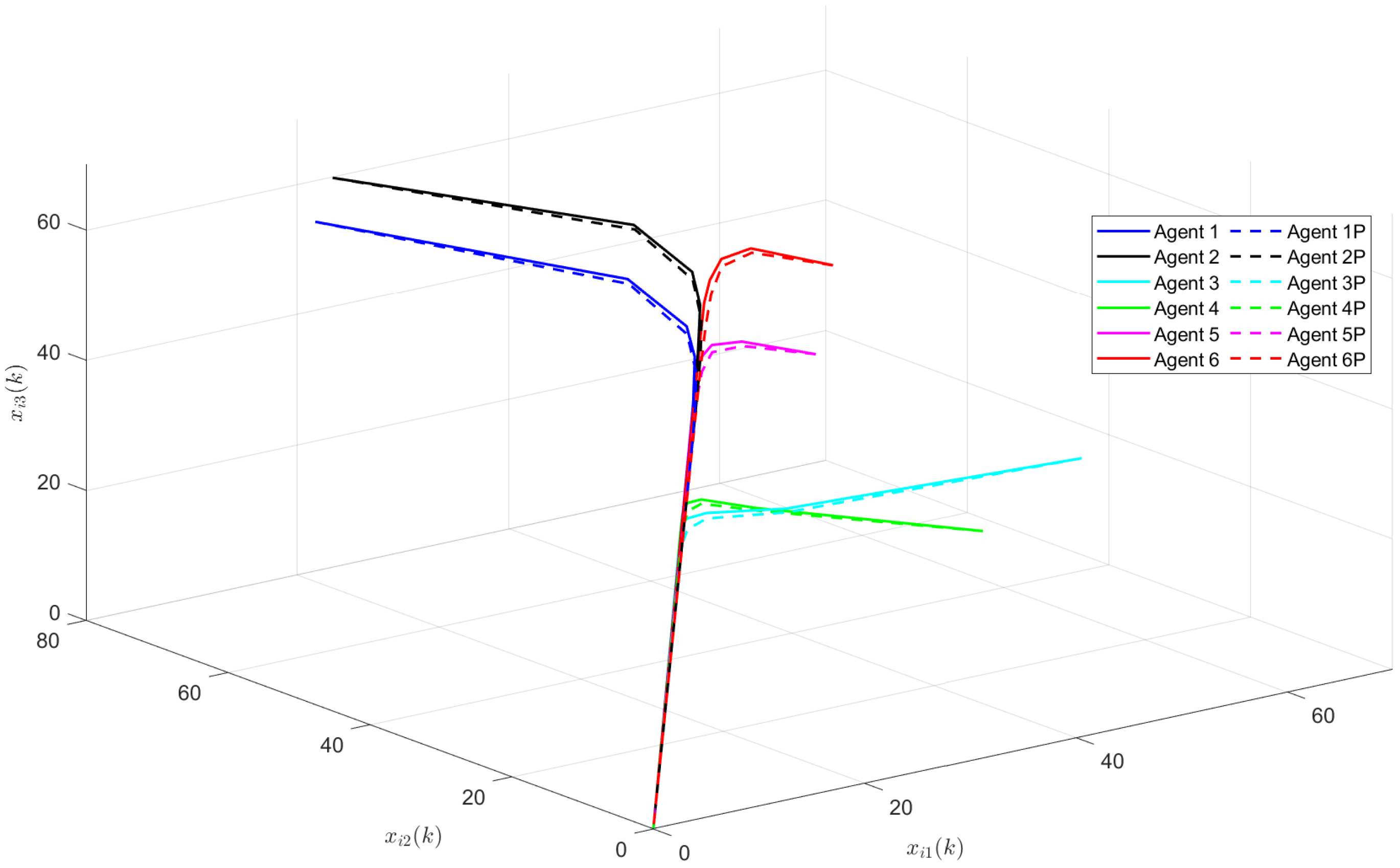
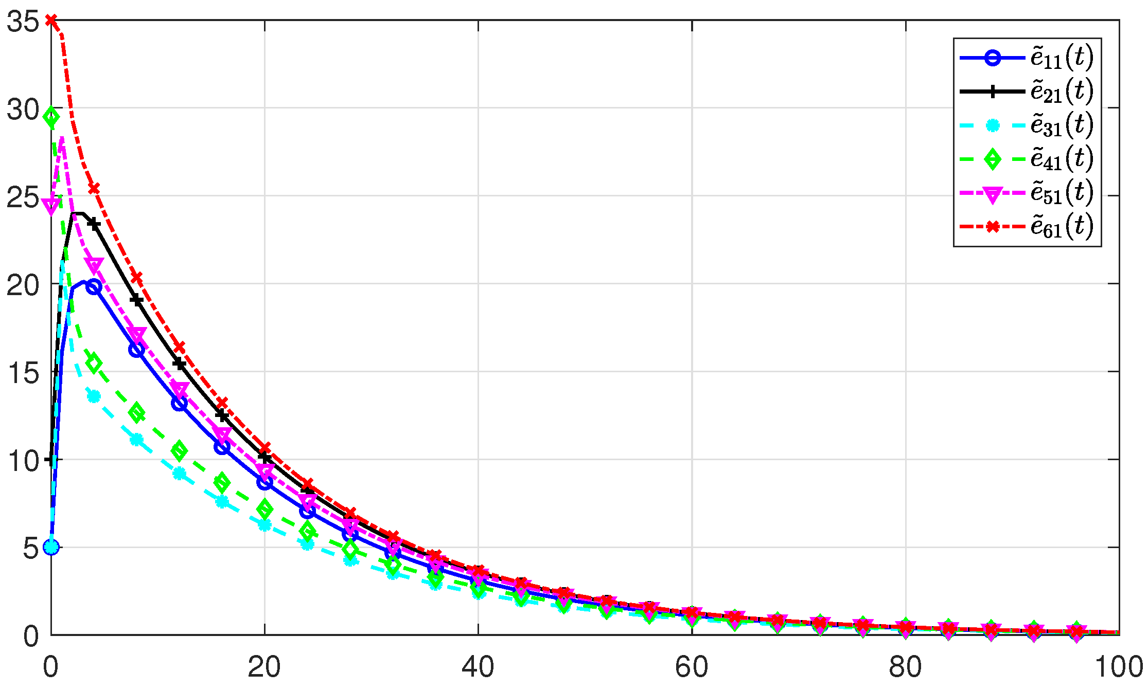
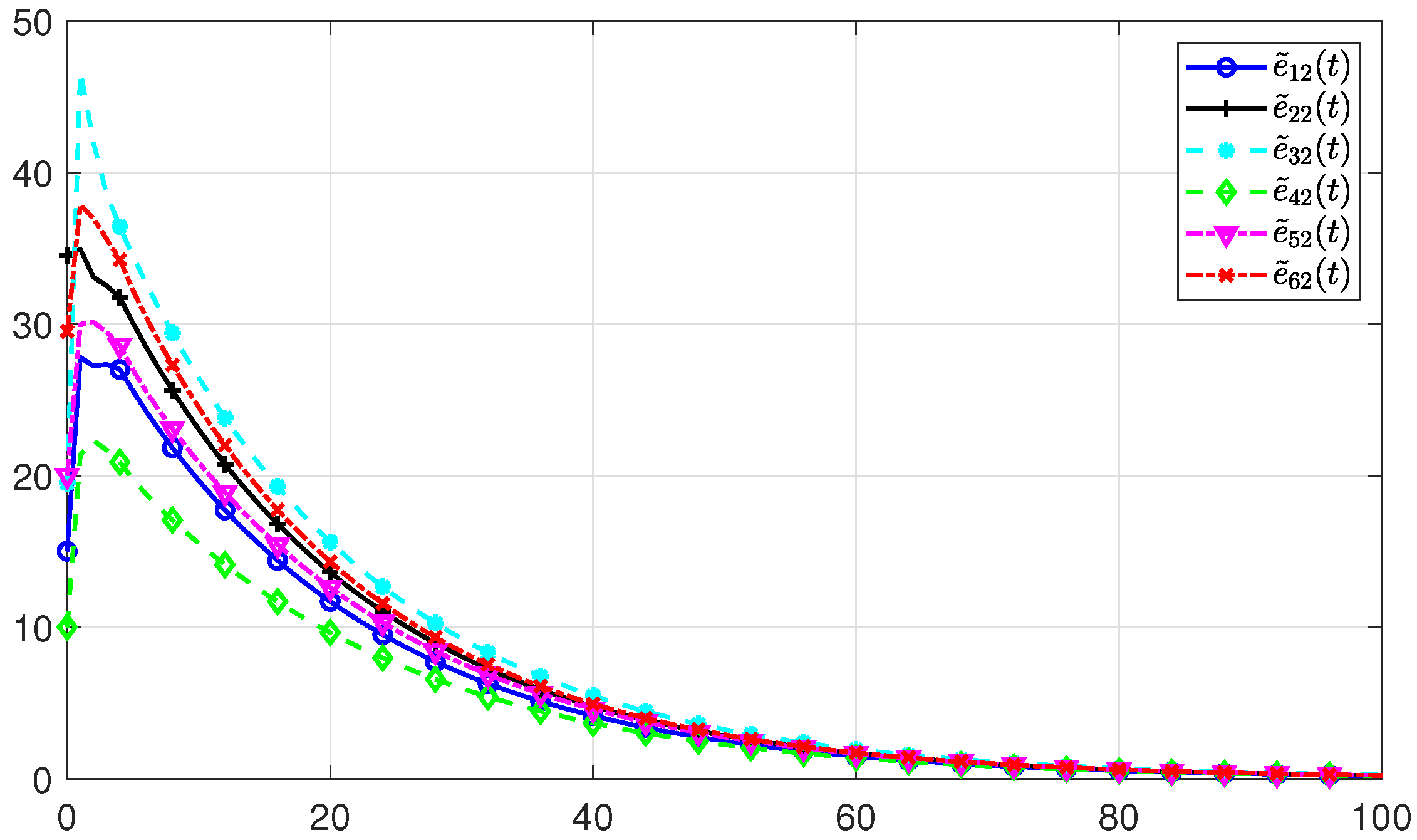
4. Illustrative Examples

With the fast development of information technology, the traditional industries have evolved rapidly by combining with modern smart equipment. For example, the wireless sensor networks are widely used in precise agriculture. Smart greenhouse can provide adaptive environmental conditions for plants at different growth stages. For different plants or plants of different stages, the requirements for climate environments, fertilizer environments, and irrigation environments are distinctive. Therefore, the climate control, fertilization control, and irrigation control are vital for the growth of plants. To obtain suitable growth environments, an efficient control protocol is key to solve the control problems. Since the data about climate states, fertilization states, and irrigation states of greenhouse are always nonnegative, it is suitable to model the wireless sensor network as PMASs. A simple structure of the wireless sensor network for greenhouse is shown in Figure 2. System (2) with observer (8) can be employed to describe the comprehensive environments dynamic of a greenhouse, where $x_i\left(k\right)$ represents the real states of the greenhouse environments around of the ith sensors at time k, ${\widehat{x}}_i\left(k\right)$ is the monitoring data of time k captured by the ith sensor unit, and $u_i\left(k\right)$ indicates the control input for the surrounding environments of ith node. The sensor units capture the microclimate states at time k to estimate the microclimate states of the whole greenhouse. Based on the estimated states, different kinds of control units execute corresponding operations. Under the designed observer-based PID protocol, the greenhouse environment states will converge to a preset value.

Example 1.

To estimate the microclimate states of a smart greenhouse, the wireless sensor network is modeled as PMASs. If the estimate errors converge to zero, then the designed observer gives effective estimates. Consider the modeled system described in the form of (2) with the system matrices:

$$A=\left(\begin{array}{ccc}0.5182& 0.1452& 0.1034\\ 0.2421& 0.5878& 0.1492\\ 0.2145& 0.2492& 0.6888\end{array}\right),B=\left(\begin{array}{cc}0.04532& 0.04213\\ 0.03645& 0.05127\\ 0.02654& 0.06313\end{array}\right),C=\left(\begin{array}{ccc}0.067& 0.076& 0.077\\ 0.046& 0.064& 0.095\end{array}\right).$$

Suppose there are three agents in the PMASs, and the initial states, initial upper state estimates, and initial lower state estimates of each agent are given as: $x_1\left(0\right)={(56.0,75.0,65.0)}^{\top }$, $x_2\left(0\right)={(45.0,60.0,78.0)}^{\top }$, $x_3\left(0\right)={(64.0,52.0,80.0)}^{\top }$, ${\overline{\widehat{x}}}_1\left(0\right)={(75.0,83.0,70.0)}^{\top }$, ${\overline{\widehat{x}}}_2\left(0\right)={(48.0,64.0,80.0)}^{\top }$, ${\overline{\widehat{x}}}_3\left(0\right)={(66.0,58.0,81.0)}^{\top }$, ${\underline{\widehat{x}}}_1\left(0\right)={(45.0,63.0,60.0)}^{\top }$, ${\underline{\widehat{x}}}_2\left(0\right)={(38.0,54.0,70.0)}^{\top }$, ${\underline{\widehat{x}}}_3\left(0\right)={(56.0,48.0,71.0)}^{\top }$, respectively. The estimate errors with regard to the lower and upper initial estimates are denoted by ${\underline{e}}_i\left(k\right)$ and ${\overline{e}}_i\left(k\right)$, respectively. Based the feasible solutions of the conditions in Theorem 1, the gain matrix of the positive state observer can be obtained as $L=\left(\begin{array}{cc}0.19022& 0.17811\\ 0.20732& 0.19628\\ 0.21367& 0.20755\end{array}\right).$

Figure 3, Figure 4 and Figure 5 show the simulations and state estimations of three agents, respectively. It can be seen that the designed observer (3) provides precise estimations of the states of system (2). On the other hand, all the evolution of the real states are kept nonnegative and always between the estimated states ${\underline{x}}_i\left(k\right)$ and ${\overline{x}}_i\left(k\right)$. The simulation results of the estimate errors ${\underline{e}}_i\left(k\right)$ and ${\overline{e}}_i\left(k\right)$ of the ith agent are shown in Figure 6, Figure 7 and Figure 8, respectively. It is obvious that all the estimate errors converge asymptotically to zero, which means that the observer (3) gives effective estimates.

Example 2.

Consider a smart greenhouse wireless sensor network with six agents and the communication typology between them is undirected. It is shown in Figure 9. The adjacency matrix and the corresponding Laplacian matrix are described as:

$$\mathcal{A}=\left(\begin{array}{cccccc}0& 1& 1& 1& 0& 0\\ 1& 0& 0& 1& 1& 0\\ 1& 0& 0& 0& 0& 1\\ 1& 1& 0& 0& 0& 1\\ 0& 1& 0& 0& 0& 1\\ 0& 0& 1& 1& 1& 0\end{array}\right),\mathcal{L}=\left(\begin{array}{cccccc}3& -1& -1& -1& 0& 0\\ -1& 3& 0& -1& -1& 0\\ -1& 0& 2& 0& 0& -1\\ -1& -1& 0& 3& 0& -1\\ 0& -1& 0& 0& 2& -1\\ 0& 0& -1& -1& -1& 3\end{array}\right).$$

The systems matrices of the PMASs are given as:

$$A=\left(\begin{array}{ccc}0.47& 0.24& 0.15\\ 0.34& 0.52& 0.21\\ 0.21& 0.3& 0.57\end{array}\right),B=\left(\begin{array}{cc}0.01& 0.02\\ 0.02& 0.04\\ 0.02& 0.01\end{array}\right),C=\left(\begin{array}{ccc}0.47& 0.9& 0.66\\ 0.81& 0.57& 0.95\end{array}\right).$$

The eigenvalues of matrix A are 1.0002, 0.20459, 0.35524, which means that matrix A is not Schur, i.e., the consensus of the PMASs (2) cannot be reached without a suitable control protocol. Then the essential objective to be achieved is that the consensus of the PMASs can be reached under the constructed PID protocol (9) with the designed observer (8).

Give the initial states and initial estimated states of all the agents as: $x_1\left(0\right)={(45.0,70.0,60.0)}^{\top }$, $x_2\left(0\right)={(50.0,75.0,63.0)}^{\top }$, $x_3\left(0\right)={(54.0,80.0,70.0)}^{\top }$, $x_4\left(0\right)={(50.0,48.0,57.0)}^{\top }$, $x_5\left(0\right)={(55.0,59.0,60.0)}^{\top }$, $x_6\left(0\right)={(62.0,67.0,68.0)}^{\top }$, ${\widehat{x}}_1\left(0\right)={(42.0,68.0,57.0)}^{\top }$, ${\widehat{x}}_2\left(0\right)={(46.0,65.5,61.5)}^{\top }$, ${\widehat{x}}_3\left(0\right)={(52.0,78.5,67.0)}^{\top }$, ${\widehat{x}}_4\left(0\right)={(46.5,47.0,55.5)}^{\top }$, ${\widehat{x}}_5\left(0\right)={(54.5,53.0,52.5)}^{\top }$, ${\widehat{x}}_6\left(0\right)={(61.0,62.5,62.0)}^{\top }$. Choose ${\lambda }_1=20,{\lambda }_2=1.1,d=3$. By solving the conditions presented in Theorem 2, the gain matrices E and L of observer (8) are

$$E=\left(\begin{array}{ccc}0.082367& 0.022521& 0.017457\\ 0.041526& 0.077002& 0.019743\\ 0.024487& 0.056101& 0.083519\end{array}\right),L=\left(\begin{array}{cc}0.024837& 0.021941\\ 0.039995& 0.027281\\ 0.049581& 0.038219\end{array}\right).$$

Similarly, the gain matrices $K_S,K_P,K_I$, and $K_D$ of the designed PID protocol (9) can be calculated as:

$$\begin{array}{c}{K}_S=\left(\begin{array}{ccc}-3.0821& -3.3926& -1.871\\ -3.094& -3.4333& -1.7997\end{array}\right),K_P=\left(\begin{array}{ccc}-0.26226& -0.29183& -0.1506\\ -0.26728& -0.33059& -0.06566\end{array}\right),\\ K_I=\left(\begin{array}{ccc}0.17265& 0.18773& 0.10017\\ 0.17224& 0.18687& 0.10153\end{array}\right),K_D=\left(\begin{array}{ccc}-0.18887& -0.20327& -0.062235\\ -0.19402& -0.21623& -0.041476\end{array}\right).\end{array}$$

The simulation results of the PMASs (2) under the observer-based PID control mechanism (9) and the observer-based hierarchical protocol (26) are depicted in Figure 10. The solid line represents the simulations of the state trajectory under the observer-based PID protocol, and the dotted line represents the hierarchical protocol. It can be seen from Figure 10 that all the states converge to zero under both protocols. Consequently, it is not hard to get that the consensus of PMASs (2) can be reached. However, it is easy to see that the state trajectory under the PID protocol converges faster than under the hierarchical protocol, which proves the superiority of the designed observer-based PID protocol. The estimate errors of all agents are shown in Figure 11, Figure 12 and Figure 13. We can see that all the estimate errors keep nonnegative and converge to zero, which implies that the designed observer (3) performs an accurate observation.

It is well known that the potential noise may be amplified by the derivative component on PID controllers. To survey the sensibility of the designed PID protocol on the derivative component, a gain disturbance has been added, which is denoted by $\Delta K_D$. Thus, the gain matrix of the derivative component can be given as $K_D+\Delta K_D$. For clarity, we define that all entries of $\Delta K_D$ are ϖ. Figure 14 illustrates the state trajectory of all the agents with different disturbances of component D. It can be seen that after the disturbance is added, the system fluctuates and takes more time to reach an agreement. Figure 15 shows the simulation of the estimation error of the second component of each agent state. It reveals that when the disturbance exceeds a certain bound, negative estimation error occurs. It means that the positivity of the closed-loop system (11) cannot be guaranteed.

5. Conclusions

In this paper, the observer-based PID control protocol for the consensus problem of PMASs is investigated. First, a kind of observer is developed by extending the observer of general positive systems into the PMASs. The introduced observer can be used to design the lower and upper state boundaries of the PMASs. Second, an improved observer with less conservatism is constructed and then the observer-based PID control protocol is proposed. The consensus issue of PMASs has been resolved under the designed PID protocol. Third, the proposed observer-based PID control protocol is expanded to deal with the consensus of heterogeneous PMASs. Moreover, all the conditions presented in this paper can be solved in terms of linear programming. Finally, the simulation results have validated the correctness of proposed design.

The future research will mainly be carried out from the following aspects. First, some performances on the observer-based PID protocols will be considered, such as robustness, stabilization time, stabilization region, etc. Second, more advanced controllers should be taken into consideration for PMASs. Third, the observer design may be improved to guarantee the separate design principle of the observer and controller gain matrices.

References

1. McArthur, S.D.; Davidson, E.M.; Catterson, V.M.; Dimeas, A.L.; Hatziargyriou, N.D.; Ponci, F.; Funabashi, T. Multi-Agent Systems for Power Engineering Applications—Part II: Technologies, Standards, and Tools for Building Multi-Agent Systems. IEEE Trans. Power Syst. 2007, 22, 1753–1759. [Google Scholar] [CrossRef] [Green Version]
2. Sujil, A.; Verma, J.; Kumar, R. Multi Agent System: Concepts, Platforms and Applications in Power Systems. Artif. Intell. Rev. 2018, 49, 153–182. [Google Scholar] [CrossRef]
3. Lee, J.H.; Kim, C.O. Multi-Agent Systems Applications in Manufacturing Systems and Supply Chain Management: A Review Paper. Int. J. Prod. Res. 2008, 46, 233–265. [Google Scholar] [CrossRef]
4. Dudek, G.; Jenkin, M.R.; Milios, E.; Wilkes, D. A Taxonomy for Multi-Agent Robotics. Auton. Robots 1996, 3, 375–397. [Google Scholar] [CrossRef]
5. Ota, J. Multi-Agent Robot Systems as Distributed Autonomous Systems. Adv. Eng. Inform. 2006, 20, 59–70. [Google Scholar] [CrossRef]
6. Afrin, M.; Jin, J.; Rahman, A.; Rahman, A.; Wan, J.; Hossain, E. Resource Allocation and Service Provisioning in Multi-Agent Cloud Robotics: A Comprehensive Survey. IEEE Commun. Surv. Tutor. 2021, 23, 842–870. [Google Scholar] [CrossRef]
7. Cai, J.; Kim, D.; Jaramillo, R.; Braun, J.E.; Hu, J. A General Multi-Agent Control Approach for Building Energy System Optimization. Energy Build. 2016, 127, 337–351. [Google Scholar] [CrossRef] [Green Version]
8. González-Briones, A.; De La Prieta, F.; Mohamad, M.S.; Omatu, S.; Corchado, J.M. Multi-Agent Systems Applications in Energy Optimization Problems: A State-of-the-Art Review. Energies 2018, 11, 1928. [Google Scholar] [CrossRef] [Green Version]
9. Dong, G.; Li, H.; Ma, H.; Lu, R. Finite-Time Consensus Tracking Neural Network FTC of Multi-Agent Systems. IEEE Trans. Neural Netw. Learn. Syst. 2020, 32, 653–662. [Google Scholar] [CrossRef]
10. Li, X.M.; Zhou, Q.; Li, P.; Li, H.; Lu, R. Event-Triggered Consensus Control for Multi-Agent Systems against False Data-Injection Attacks. IEEE Trans. Cybern. 2019, 50, 1856–1866. [Google Scholar] [CrossRef]
11. Ma, Z.; Wang, Y.; Li, X. Cluster-Delay Consensus in First-Order Multi-Agent Systems with Nonlinear Dynamics. Nonlinear Dyn. 2016, 83, 1303–1310. [Google Scholar] [CrossRef]
12. Valcher, M.E.; Misra, P. On the Stabilizability and Consensus of Positive Homogeneous Multi-Agent Dynamical Systems. IEEE Trans. Autom. Control 2014, 59, 1936–1941. [Google Scholar] [CrossRef]
13. Su, H.; Wu, H.; Chen, X.; Chen, M.Z.Q. Positive Edge Consensus of Complex Networks. IEEE Trans. Syst. Man Cybern. Syst. 2018, 48, 2242–2250. [Google Scholar] [CrossRef]
14. Ren, W.; Atkins, E. Distributed Multi-Vehicle Coordinated Controlvia Local Information Exchange. Int. J. Robust Nonlinear Control 2007, 17, 1002–1033. [Google Scholar] [CrossRef] [Green Version]
15. Pahuja, R.; Verma, H.; Uddin, M. A Wireless Sensor Network for Greenhouse Climate Control. IEEE Pervasive Comput. 2013, 12, 49–58. [Google Scholar] [CrossRef]
16. Silva, P.C.; Batista, P.V.; Lima, H.S.; Alves, M.A.; Guimarães, F.G.; Silva, R.C. COVID-ABS: An Agent-Based Model of COVID-19 Epidemic to Simulate Health and Economic Effects of Social Distancing Interventions. Chaos Solitons Fractals 2020, 139, 110088. [Google Scholar] [CrossRef]
17. Rami, M.A.; Tadeo, F. Controller Synthesis for Positive Linear Systems With Bounded Controls. IEEE Trans. Circuits Syst. II Express Briefs 2007, 54, 151–155. [Google Scholar] [CrossRef]
18. Xiang, M.; Xiang, Z. Stability, L1-gain and Control Synthesis for Positive Switched Systems with Time-Varying Delay. Nonlinear Anal. Hybrid Syst. 2013, 9, 9–17. [Google Scholar] [CrossRef]
19. Shen, J.; Lam, J. L -Gain Analysis for Positive Systems with Distributed Delays. Automatica 2014, 50, 175–179. [Google Scholar] [CrossRef]
20. Zhang, J.; Zheng, G.; Feng, Y.; Chen, Y. Event-Triggered State-Feedback and Dynamic Output-Feedback Control of Positive Markovian Jump Systems With Intermittent Faults. IEEE Trans. Autom. Control 2022. [Google Scholar] [CrossRef]
21. Zhang, J.; Zhang, S.; Deng, X.; Huang, Z. Adaptive Event-Triggered Dynamic Distributed Control of Switched Positive Systems with Switching Faults. Nonlinear Anal. Hybrid Syst. 2023, 48, 101328. [Google Scholar] [CrossRef]
22. Nguyen, A.T.; Taniguchi, T.; Eciolaza, L.; Campos, V.; Palhares, R.; Sugeno, M. Fuzzy Control Systems: Past, Present and Future. IEEE Comput. Intell. Mag. 2019, 14, 56–68. [Google Scholar] [CrossRef]
23. Liu, L.; Liu, Y.J.; Chen, A.; Tong, S.; Chen, C.L.P. Integral Barrier Lyapunov Function-Based Adaptive Control for Switched Nonlinear Systems. Sci. China Inf. Sci. 2020, 63, 132203. [Google Scholar] [CrossRef] [Green Version]
24. Zhang, M.; Shi, P.; Shen, C.; Wu, Z.G. Static Output Feedback Control of Switched Nonlinear Systems With Actuator Faults. IEEE Trans. Fuzzy Syst. 2020, 28, 1600–1609. [Google Scholar] [CrossRef]
25. Zhang, D.; Han, Q.L.; Zhang, X.M. Network-Based Modeling and Proportional–Integral Control for Direct-Drive-Wheel Systems in Wireless Network Environments. IEEE Trans. Cybern. 2020, 50, 2462–2474. [Google Scholar] [CrossRef]
26. Humaidi, A.J.; Abdulkareem, A.I. Design of Augmented Nonlinear PD Controller of Delta/Par4-Like Robot. J. Control Sci. Eng. 2019, 2019, 1–11. [Google Scholar] [CrossRef]
27. Zhao, C.; Guo, L. PID Controller Design for Second Order Nonlinear Uncertain Systems. Sci. China Inf. Sci. 2017, 60, 022201. [Google Scholar] [CrossRef] [Green Version]
28. Ang, K.H.; Chong, G.; Li, Y. PID Control System Analysis, Design, and Technology. IEEE Trans. Control Syst. Technol. 2005, 13, 559–576. [Google Scholar] [CrossRef] [Green Version]
29. Zhao, C.; Guo, L. Control of Nonlinear Uncertain Systems by Extended PID. IEEE Trans. Autom. Control 2021, 66, 3840–3847. [Google Scholar] [CrossRef]
30. Li, X.G.; Niculescu, S.I.; Chen, J.X.; Chai, T. Characterizing PID Controllers for Linear Time-Delay Systems: A Parameter-Space Approach. IEEE Trans. Autom. Control 2021, 66, 4499–4513. [Google Scholar] [CrossRef]
31. Yu, H.; Guan, Z.; Chen, T.; Yamamoto, T. Design of Data-Driven PID Controllers with Adaptive Updating Rules. Automatica 2020, 121, 109185. [Google Scholar] [CrossRef]
32. Lui, D.G.; Petrillo, A.; Santini, S. An Optimal Distributed PID-like Control for the Output Containment and Leader-Following of Heterogeneous High-Order Multi-Agent Systems. Inf. Sci. 2020, 541, 166–184. [Google Scholar] [CrossRef]
33. De Tommasi, G.; Lui, D.G.; Petrillo, A.; Santini, S. A L2-gain Robust PID-like Protocol for Time-varying Output Formation-containment of Multi-agent Systems with External Disturbance and Communication Delays. IET Control Theory Appl. 2021, 15, 1169–1184. [Google Scholar] [CrossRef]
34. Yu, X.; Yang, F.; Zou, C.; Ou, L. Stabilization Parametric Region of Distributed PID Controllers for General First-Order Multi-Agent Systems With Time Delay. IEEE-CAA J. Autom. Sin. 2020, 7, 1555–1564. [Google Scholar] [CrossRef]
35. Li, Z.; Ren, W.; Liu, X.; Fu, M. Consensus of Multi-Agent Systems with General Linear and Lipschitz Nonlinear Dynamics Using Distributed Adaptive Protocols. IEEE Trans. Autom. Control 2013, 58, 1786–1791. [Google Scholar] [CrossRef] [Green Version]
36. Valcher, M.E.; Zorzan, I. On the Consensus of Homogeneous Multiagent Systems With Positivity Constraints. IEEE Trans. Autom. Control 2017, 62, 5096–5110. [Google Scholar] [CrossRef]
37. Liu, J.J.R.; Lam, J.; Kwok, K.W. Positive Consensus of Fractional-Order Multiagent Systems Over Directed Graphs. IEEE Trans. Neural Netw. Learn. Syst. 2022, 1–7. [Google Scholar] [CrossRef]
38. Samad, T. A Survey on Industry Impact and Challenges Thereof. IEEE Control Syst. Mag. 2017, 37, 17–18. [Google Scholar] [CrossRef]
39. Li, Z.; Duan, Z.; Chen, G. Consensus of Discrete-Time Linear Multi-Agent Systems with Observer-Type Protocols. Discrete Contin. Dyn. Syst. 2011, 16, 489–505. [Google Scholar] [CrossRef] [Green Version]
40. Cai, H.; Lewis, F.L.; Hu, G.; Huang, J. The Adaptive Distributed Observer Approach to the Cooperative Output Regulation of Linear Multi-Agent Systems. Automatica 2017, 75, 299–305. [Google Scholar] [CrossRef]
41. You, R.; Tang, M.; Guo, S.; Cui, G. Proportional Integral Observer-based Consensus Control of Discrete-time Multi-agent Systems. Int. J. Control Autom. Syst. 2022, 20, 1461–1472. [Google Scholar] [CrossRef]
42. Gong, X.; Liu, J.; Wang, Y.; Lam, J. Consensus of Discrete-time Positive Multi-agent Systems with Observer-type Protocols. In Proceedings of the 2019 IEEE 15th International Conference on Control and Automation (ICCA), Edinburgh, UK, 16–19 July 2019; IEEE: Edinburgh, UK, 2019; pp. 846–850. [Google Scholar] [CrossRef]
43. Wu, H.; Su, H. Observer-Based Consensus for Positive Multiagent Systems With Directed Topology and Nonlinear Control Input. IEEE Trans. Syst. Man Cybern. Syst. 2019, 49, 1459–1469. [Google Scholar] [CrossRef]
44. Liu, J.J.R.; Lam, J.; Wang, Y.; Cui, Y.; Shu, Z. Robust and Nonfragile Consensus of Positive Multiagent Systems via Observer-based Output-feedback Protocols. Int. J. Robust Nonlinear Control 2020, 30, 5386–5403. [Google Scholar] [CrossRef]
45. Chen, S.; An, Q.; Zhou, H.; Su, H. Observer-Based Consensus for Fractional-Order Multi-Agent Systems with Positive Constraint. Neurocomputing 2022, 501, 489–498. [Google Scholar] [CrossRef]
46. Farina, L.; Rinaldi, S. Positive Linear Systems: Theory and Applications; John Wiley & Sons: Hoboken, NJ, USA, 2000; Volume 50. [Google Scholar]
47. Kaczorek, T. Positive 1D and 2D Systems; Springer Science & Business Media: Berlin/Heidelberg, Germany, 2002. [Google Scholar]
48. Rami, M.A.; Tadeo, F. Positive Observation Problem for Linear Discrete Positive Systems. In Proceedings of the 45th IEEE Conference on Decision and Control, San Diego, CA, USA, 13–15 December 2006; pp. 4729–4733. [Google Scholar] [CrossRef]
49. Zhang, J.; Zhang, R.; Chen, Y.; Fu, S. Linear Programming Based Dynamic Output-Feedback Controller for Positive Systems. In Proceedings of the 2017 American Control Conference (ACC), Seattle, WA, USA, 24–26 May 2017; pp. 1709–1714. [Google Scholar] [CrossRef]
50. Luenberger, D. An Introduction to Observers. IEEE Trans. Autom. Control 1971, 16, 596–602. [Google Scholar] [CrossRef]
51. Liu, J.J.R.; Yang, N.; Kwok, K.W.; Lam, J. Positive Consensus of Directed Multiagent Systems. IEEE Trans. Autom. Control 2022, 67, 3641–3646. [Google Scholar] [CrossRef]
52. Bhattacharyya, S.; Patra, S. Positive Consensus of Multi-Agent Systems with Hierarchical Control Protocol. Automatica 2022, 139, 110191. [Google Scholar] [CrossRef]
53. Cao, X.; Li, Y. Positive Consensus for Multi-Agent Systems with Average Dwell Time Switching. J. Frankl. Inst. 2021, 358, 8308–8329. [Google Scholar] [CrossRef]
54. Yang, N.; Yin, Y.; Liu, J. Positive Consensus of Directed Multi-agent Systems Using Dynamic Output-feedback Control. In Proceedings of the 2019 IEEE 58th Conference on Decision and Control (CDC), Nice, France, 11–13 December 2019; pp. 897–902. [Google Scholar] [CrossRef]
55. Sun, Y.; Su, H.; Wang, X.; Chen, S. Semi-global Edge-consensus of Linear Discrete-time Multi-agent Systems with Positive Constraint and Input Saturation. IET Control Theory Appl. 2019, 13, 979–987. [Google Scholar] [CrossRef]
56. Gionfra, N.; Sandou, G.; Siguerdidjane, H.; Faille, D. A Distributed PID-like Consensus Control for Discrete-time Multi-agent Systems. In Proceedings of the 14th International Conference on Informatics in Control, Automation and Robotics, Madrid, Spain, 26–28 July 2017; pp. 72–81. [Google Scholar] [CrossRef]
57. Li, J.; Wang, J. Reinforcement Learning Based Proportional–Integral–Derivative Controllers Design for Consensus of Multi-Agent Systems. ISA Trans. 2022, in press. [Google Scholar] [CrossRef]
58. Zheng, Y.; Wang, L.; Zhu, Y. Consensus of Heterogeneous Multi-Agent Systems. IET Control Theory Appl. 2011, 5, 1881–1888. [Google Scholar] [CrossRef]
59. Zheng, Y.; Wang, L. Containment Control of Heterogeneous Multi-Agent Systems. Int. J. Control 2014, 87, 1–8. [Google Scholar] [CrossRef]
60. Ma, Q.; Miao, G. Output Consensus for Heterogeneous Multi-Agent Systems with Linear Dynamics. Appl. Math. Comput. 2015, 271, 548–555. [Google Scholar] [CrossRef]
61. Zuo, S.; Song, Y.; Lewis, F.L.; Davoudi, A. Output Containment Control of Linear Heterogeneous Multi-Agent Systems Using Internal Model Principle. IEEE Trans. Cybern. 2017, 47, 2099–2109. [Google Scholar] [CrossRef]
Figure 1. Block diagram of agent i with observer-based control.
Mathematics 11 00419 g001
Figure 2. The structure of smart greenhouse.
Mathematics 11 00419 g002
Figure 3. The simulations of all states and their estimations of the first agent.
Mathematics 11 00419 g003
Figure 4. The simulations of all states and their estimations of the 2nd agent.
Mathematics 11 00419 g004
Figure 5. The simulations of all states and their estimations of the 3rd agent.
Mathematics 11 00419 g005
Figure 6. The simulations of state estimate errors e 1 ( k ) of the 1st agent.
Mathematics 11 00419 g006
Figure 7. The simulations of state estimate errors e 2 ( k ) of the 2nd agent.
Mathematics 11 00419 g007
Figure 8. The simulations of state estimate errors e 3 ( k ) of the 3th agent.
Mathematics 11 00419 g008
Figure 9. Communication typology.
Mathematics 11 00419 g009
Figure 10. The simulations of states of all the agents.
Mathematics 11 00419 g010
Figure 11. The simulations of e ˜ i 1 ( k ) of all the agents.
Mathematics 11 00419 g011
Figure 12. The simulation of e ˜ i 2 ( k ) of all the agents.
Mathematics 11 00419 g012
Figure 13. The simulations of e ˜ i 3 ( k ) of all the agents.
Mathematics 11 00419 g013
Figure 14. The state trajectory of all the agents with different disturbances of component D.
Mathematics 11 00419 g014
Figure 15. The simulation of e ˜ i 2 ( k ) with different disturbances of component D.
Mathematics 11 00419 g015
Disclaimer/Publisher’s Note: The statements, opinions and data contained in all publications are solely those of the individual author(s) and contributor(s) and not of MDPI and/or the editor(s). MDPI and/or the editor(s) disclaim responsibility for any injury to people or property resulting from any ideas, methods, instructions or products referred to in the content.