Article

Efficient Associate Rules Mining Based on Topology for Items of Transactional Data

1
School of Computer and Software Engineering, Xihua University, Chengdu 610039, China
2
School of Science, Xihua University, Chengdu 610039, China
3
Intelligent Policing Key Laboratory of Sichuan Province, Sichuan Police College, Luzhou 646000, China
4
School of Computer Science, Shaanxi Normal University, Xi’an 710119, China
*
Authors to whom correspondence should be addressed.
Mathematics 2023, 11(2), 401; https://doi.org/10.3390/math11020401
Submission received: 9 December 2022 / Revised: 1 January 2023 / Accepted: 7 January 2023 / Published: 12 January 2023
(This article belongs to the Special Issue Artificial Intelligence and Data Science)

Abstract

:
A challenge in association rules’ mining is effectively reducing the time and space complexity in association rules mining with predefined minimum support and confidence thresholds from huge transaction databases. In this paper, we propose an efficient method based on the topology space of the itemset for mining associate rules from transaction databases. To do so, we deduce a binary relation on itemset, and construct a topology space of itemset based on the binary relation and the quotient lattice of the topology according to transactions of itemsets. Furthermore, we prove that all closed itemsets are included in the quotient lattice of the topology, and generators or minimal generators of every closed itemset can be easily obtained from an element of the quotient lattice. Formally, the topology on itemset represents more general associative relationship among items of transaction databases, the quotient lattice of the topology displays the hierarchical structures on all itemsets, and provide us a method to approximate any template of the itemset. Accordingly, we provide efficient algorithms to generate Min-Max association rules or reduce generalized association rules based on the lower approximation and the upper approximation of a template, respectively. The experiment results demonstrate that the proposed method is an alternative and efficient method to generate or reduce association rules from transaction databases.

1. Introduction

In knowledge discovery in database (KDD), association rules mining (ARM) from transaction databases proposed in [1,2] have received considerable attention and wide applications, such as medical diagnosis [3,4], marketing planning [5,6], etc. ARM can be formally explained as follows: Let A = ( U , A ) be a transaction database, where U a non-empty finite set of transactions, A a non-empty finite set of items, each transaction u i U decides a mapping u i : A { 0 , 1 } , i.e., for any item a j A , the transaction u i has (or has not) the item a j A if u i ( a j ) = 1 (or u i ( a j ) = 0 ), each subset of A is called as an itemset. An association rule describing the co-occurrence relation among items is an implication in the form A 1 A 2 , where itemsets A 1 and A 2 of A such that A 1 A 2 = are called as antecedent and consequent, respectively. Theoretically, ARM from a transaction database is a NP-hard problem because itemsets A 1 and A 2 are selected from 2 | A | (powerset of A), in real world practices, the existed mining methods usually extract a large number of association rules which are difficult to handle; many kinds of association rules or mining methods have been proposed to generate association rules, although these mining methods are different, their processing is nearly the same, i.e., how to evaluate usefulness of association rules and how to select the antecedent and consequent of association rules.
Quality measures are used to evaluate the usefulness of association rules, and various measures have been provided to discover significant and specific association rules. In a transaction database A = ( U , A ) , for any A A , denote τ ( A ) = { u i U | a j A , u i ( a j ) = 1 } , ¬ A is the absence of A , then the following quality measures can be defined
  • Support [1,2]: s u p p A ( A 1 A 2 ) = | τ ( A 1 A 2 ) | | U | ;
  • Confidence [1,2]: c o n f A ( A 1 A 2 ) = s u p p A ( A 1 A 2 ) s u p p A ( A 1 ) ;
  • Netconfidence [7]: n e t c A ( A 1 A 2 ) = s u p p A ( A 1 A 2 ) s u p p A ( A 1 ) s u p p A ( A 2 ) s u p p A ( A 1 ) ( 1 s u p p A ( A 1 ) ) ;
  • Conviction [8]: c o n v A ( A 1 A 2 ) = s u p p A ( A 1 ) s u p p A ( ¬ A 2 ) s u p p A ( A 1 ¬ A 2 ) ;
  • Added value [9]: a d d A ( A 1 A 2 ) = c o n f A ( A 1 A 2 ) s u p p A ( A 2 ) ;
  • Accuracy [9]: a c c A ( A 1 A 2 ) = c o n f A ( A 1 A 2 ) + c o n f A ( ¬ A 1 ¬ A 2 ) ;
  • Interestingness [10]: i n t e A ( A 1 A 2 ) = s u p p A ( A 1 A 2 ) s u p p A ( A 1 ) × s u p p A ( A 1 A 2 ) s u p p A ( A 2 ) × ( 1 s u p p A ( A 1 A 2 ) ) ;
  • Comprehensibility [10]: c o m p A ( A 1 A 2 ) = log ( 1 + | τ ( A 2 ) | ) log ( 1 + | τ ( A 1 A 2 ) | ) ;
  • Lift [11]: l i f t A ( A 1 A 2 ) = s u p p A ( A 1 A 2 ) s u p p A ( A 1 ) s u p p A ( A 2 ) .
By combining with several quality measures to form fitness functions, ARM is transformed into optimization problems, and various optimal algorithms can be used to extract interesting or valid association rules from A = ( U , A ) . In [12], schema constraints and the opportunistic confidence constraint are enforced to mine generalized association rules in the analyzed data. In [13], confidence, comprehensibility, and interestingness are considered as a multi-objective problem, and the particle swarm optimization algorithm is proposed to extract the best rules. In [10], support, comprehensibility and interestingness are considered as a multi-objective problem, and a Pareto-based genetic algorithm is used to extract some useful and interesting rules from any market-basket type database. In [14], Shafer’s theory of evidence is used as two information measures for the quality evaluation of the set of frequent itemset (or frequent pattern). In [15], off-the-shelf constraint programming techniques are employed for modeling and solving a wide variety of constraint-based frequent itemsets. In [16], based on exclusive causal-leverage measure, a data mining algorithm is developed to mine the causal relation between drugs and their associated adverse drug reactions. In [17], the particle swarm optimization algorithm are provided to improve computational efficiency as well as to automatically determine suitable support and confidence threshold values of association rules. In [18], grammar-guided genetic programming models are proposed to deal with the association rule mining problem under a multi-objective perspective. In [19], a new multi-objective evolutionary model, which maximizes the comprehensibility, interestingness and performance of the objectives, is presented to mine a set of quantitative association rules with a good trade-off between interpretability and accuracy. In [20], a principal components analysis is applied to a set of measures that evaluate quantitative association rules’ quality; the QARGA algorithm is provided to find out quantitative association rules from a wide variety of datasets. In [21], a new confidence degree of association rules and a discrete bi-level parametric programming are proposed to extract association rules from huge databases. In [22], redundancy analysis, sampling and multivariate statistical analysis are provided to ascertain the discovered rules and discard the non-significant rules. In [23], a systematic assessment of various numerical association rule mining methods and a meta-study of thirty numerical association rule mining algorithms are provided. The authors investigate how far the discretization techniques have been used in the numerical association rule mining methods. In [24], a multi-objective particle swarm optimization is proposed using an adaptive archive grid based on the Pareto optimal strategy for numerical association rule mining. In [25,26,27,28], these papers adopt the idea of parallelization and improves the Apriori algorithm based on the MapReduce model.
By analyzing associative relation among items, suitable itemsets can be selected to generate association rules. The most widely used itemsets are frequent itemsets and closed itemsets [15,29,30,31,32], an itemset is frequent if its support is not less than the minimum support value, an itemset is closed if and only if no proper superset of the itemset has the same support as the itemset. In [33], frequent itemsets are employed to construct taxonomy over items, and a breadth-first search is adopted to enumerate all frequent itemsets. Closed frequent itemsets can be used to uniquely determine the set of all frequent itemsets and applied to generate a condensed set of association rules [34,35,36]. Formally, all closed itemsets of A = ( U , A ) can be constructed as a closed itemset lattice, and CHARM-L algorithm is proposed to explicitly generate the frequent closed itemset lattice [37]. In [38], the parent-child relation of the closed itemset lattice has been exploited, and the cross-level closed itemset lattice is constructed to mine the most relevant minimal cross-level association rules. In [39], an efficient post-processing method is presented to prune redundant rules by virtue of the property of Galois connection, which inherently constrains rules with respect to objects. At present, itemsets have been widely investigated [40,41], and various itemsets and their generating algorithms for specific association rules mining have been proposed, such as expressive generalized itemsets [42], free itemsets [43], disjunction-free itemsets [44,45], non-derivable itemsets [46,47], disjunctive closed itemsets [48], etc. In fact, we notice that frequent itemsets or closed itemsets are rooted to the co-occurrence relation among items; from the mathematical point of view, topology may be a more suitable tool to express the relation among items, because a topology for the set is used to express a relation among subsets, subsets of the set are granulated as members of the topology, and the topology for the set is generated by its topology base; this means that the base for the topology is the basic relation among elements of the set. Topology-based pattern mining has been widely investigated in the rough set theory and knowledge model, such as in [49]; a nested topology on a crisp set of reference is provided to interpret a fuzzy subset; the approach provides us a unified framework for most of the fuzzy thresholding algorithms. In [50], the lower and upper approximations of the rough set theory are shown as pre-topological invariants and dual to each other, and the corresponding generalized topological closure via the upper approximation is constructed. In [51], the knowledge representation and reasoning method are proposed for identity-based spatial change; the change process is presented by a multistage graph, the binary relation model B C for identity change is defined, and qualitative reasoning for B C and combining B C with topological relations are investigated.
In this paper, we analyze topology and the topology base for items, express more general associative relations among items and extract useful association rules based on the topology and the base; all of these are inspired by our previous works on the formal concept analysis; in [52], we proposed a novel method based on the topology for attributes of a formal context to generate all formal concepts, the topology for attributes has been used to explain the associative relation among attributes of the formal context, and the formal concept lattice can be constructed by the topology for attributes based on an equivalent relation. In [53], we used the topology for attributes of multi-valued information systems to generate Min-Max association rules. In this paper, we construct the topology for the set of items of a transaction database, which can be used to explain more general associative relation among items; moreover, we prove that frequent itemsets, closed itemsets and closed frequent itemsets are included in the topology for the set of items, provide two kinds of lattice on the topology to display the hierarchical structures on itemsets, and propose efficient algorithms based on the base for the topology to generate or reduce many kinds of association rules.
The organization of this paper is as follows: In Section 2, we briefly review some basic notions used in association rules mining. In Section 3, we present the topology for the set of items and lattices on itemsets of a transactional database, in which some important properties of the topology, the quotient lattice and minimal generators of closed frequent itemsets, are provided. In Section 4, we propose several algorithms to generate or reduce association rules, and analyze confidences of generalized association rules. In Section 5, we choose zoo, mushroom, connect-4 and chess as transactional databases to show the proposed method in generating association rules. We conclude the paper in Section 6.

2. Preliminaries

In the section, we briefly review some basic concepts used in frequent itemsets, closed itemsets or association rules mining; several concepts are also widely used in rough sets and formal concept analysis. For a uniform expression, we adopt the following set-to-set mapping in a transaction database A = ( U , A ) , denote P ( U ) and P ( A ) as power sets of U and A, respectively, then we have
τ : P ( A ) P ( U ) , τ ( A 1 ) = { u i U | a j A 1 A , u i ( a j ) = 1 } , γ : P ( U ) P ( A ) , γ ( O ) = { a j A | u i O U , u i ( a j ) = 1 } .
Based on τ and γ , we can rewrite the support of an itemset A 1 and the confidence of an association rule A 1 A 2 , as follows:
s u p p ( A 1 ) = | τ ( A 1 ) | ( o r | τ ( A 1 ) | | U | ) , c o n f ( A 1 A 2 ) = | τ ( A 1 A 2 ) | | τ ( A 1 ) | .
τ and γ also make us define closed itemsets and their generator concisely, i.e., A 1 A is a closed itemset if and only if γ τ ( A 1 ) = A 1 , an itemset A 2 is a generator of the closed itemset A 1 if and only if A 2 A 1 and γ τ ( A 2 ) = A 1 , furthermore, A 2 is a minimal generator of A 1 if and only if A 3 A 2 such that γ τ ( A 3 ) = A 1 . Formally, τ and γ are also analyzed in rough sets and formal concept analysis [50,54,55,56,57], and the following properties of τ and γ are obviously, for any A 1 , A 2 , A 3 A and O 1 , O 2 U , (1) If A 1 A 2 , then τ ( A 1 ) τ ( A 2 ) ; (2) If O 1 O 2 , then γ ( O 1 ) γ ( O 2 ) ; (3) τ ( A 1 A 2 ) = τ ( A 1 ) τ ( A 2 ) , γ ( O 1 O 2 ) = γ ( O 1 ) γ ( O 2 ) ; (4) τ ( γ τ ( A 1 ) ) = τ ( A 1 ) , γ ( τ γ ( O 1 ) ) = γ ( O 2 ) . In [52], we use τ and γ to induce a reflexive and transitive relation on the set of attributes from a formal context, the topology for attributes are constructed by using the relation, then the formal concepts are analyzed in the the topology for attributes. Here, we provide the same results in a transaction database.
Definition 1.
For any transactional database A = ( U , A ) , τ and γ decide a point-to-set mapping from A to P ( A ) , i.e., for any a i A , C : A P ( A ) is
C ( a i ) = { a j A | a j γ τ ( { a i } ) } .
Intuitively, the point-to-set mapping C represents a co-occurrence relation among items, i.e., the following binary relation on A can be decided by the mapping, C. For any a i , a j A ,
R A ( a i , a j ) = 1 , if a j C ( a i ) , 0 , if a j C ( a i ) .
In [52], we have proved that the binary relation R A on A is reflexive and transitive, and ( A , R A ) is an approximation space. For any subset A 1 of A, denote R A ̲ ( A 1 ) = { a i A | a j , ( R A ( a i , a j ) = 1 ) ( a j A 1 ) } and R A ¯ ( A 1 ) = { a i A | a j A 1 R A ( a i , a j ) = 1 } , then R A ¯ ( A 1 ) and R A ̲ ( A 1 ) are generalized upper approximation and lower approximation of A 1 , especially if R A is an equivalent relation; R A ¯ ( A 1 ) and R A ̲ ( A 1 ) are Pawlak’s upper approximation and lower approximation [55]. More important, we have the following theorem.
Theorem 1
([52]). For any transactional database A = ( U , A ) .
1 .
T ( R A ) = { R A ̲ ( A 1 ) | A 1 A } is a topology for A;
2 .
For any a i A , R A ̲ ( C ( a i ) ) = C ( a i ) ;
3 .
B A = { C ( a i ) | a i A } is a base for the topology T ( R A ) .
The theorem means that the topology for A has a simple expression, i.e., T ( R A ) = { C ( a i ) B A C ( a i ) | B A B A } , we use the following example to explain the above mentioned concepts and results; the example was initially used to analyze the concept “to-be-a-fruit” [58].
Example 1.
Let a fruit data be A = ( U , A ) , where U = { a chestnut ( u 1 ), an olive ( u 2 ), a pepper ( u 3 ), a strawberry ( u 4 ), an orange ( u 5 ), a tomato ( u 6 )} and A = { to-grow-on-trees ( a 1 ), to-be-sweet ( a 2 ), to-be-raw-edible ( a 3 ), to-yield-juice ( a 4 ), to-have-a-skin ( a 5 )} be used to understand the concept “to-be-a-fruit” (shown in Table 1). According to Definition 1, we have C ( a 1 ) = { a 1 } , C ( a 2 ) = { a 2 , a 3 } , C ( a 3 ) = { a 3 } , C ( a 4 ) = { a 3 , a 4 , a 5 } and C ( a 5 ) = { a 5 } , e.g., for C ( a 2 ) = { a 2 , a 3 } , it means that a 2 and a 3 are co-occurrence in Table 1, i.e., a fruit is “to-be-sweet”, it must be “to-be-raw-edible”. The binary relation R A on A = { a 1 , a 2 , a 3 , a 4 , a 5 } is shown in Table 2.
Based on Theorem 1 and the mapping C, we have T ( R A ) = { , { a 1 } , { a 3 } , { a 5 } , { a 1 , a 3 } , { a 1 , a 5 } , { a 2 , a 3 } , { a 3 , a 5 } , { a 1 , a 2 , a 3 } , { a 1 , a 3 , a 5 } , { a 2 , a 3 , a 5 } , { a 3 , a 4 , a 5 } , { a 1 , a 3 , a 4 , a 5 } , { a 1 , a 2 , a 3 , a 5 } , { a 2 , a 3 , a 4 , a 5 } , { a 1 , a 2 , a 3 , a 4 , a 5 } } , e.g., the member { a 2 , a 3 , a 5 } is obtained by
{ a 2 , a 3 , a 5 } = C ( a 2 ) C ( a 5 ) .
According to Table 2, we can find that R A on A is not symmetric generally, e.g., R A ( a 2 , a 3 ) = 1 but R A ( a 3 , a 2 ) = 0 , hence, members of the topology T ( R A ) for the set of items are not Pawlak’s lower approximation in practice. According to Table 1, we can obtain the support of each member in the topology for A, e.g., for { a 2 , a 3 } , we have s u p p ( { a 2 , a 3 } ) = | τ ( T ) | = | { u 4 , u 5 } | = 2 or s u p p ( { a 2 , a 3 } ) = | { u 4 , u 5 } | | U | = 1 3 . If we fix minimum support 1 3 , then members such as { a 2 , a 3 } and { a 1 , a 3 } are frequent itemsets, which can be used to generate association rules, e.g., we can generate association rules “ a 1 a 3 ” and “ a 3 a 1 ”; confidences of them are
c o n f ( a 1 a 3 ) = | τ ( { a 1 , a 3 } ) | | τ ( a 1 ) | = | { u 2 , u 5 } | | { u 1 , u 2 , u 5 } | = 2 3 , c o n f ( a 3 a 1 ) = | τ ( { a 1 , a 3 } ) | | τ ( a 3 ) | = | { u 2 , u 5 } | | { u 2 , u 3 , u 4 , u 5 , u 6 } | = 0.4 .
In A of the fruit data A = ( U , A ) , “ a 1 a 3 ” is “to-grow-on-trees implies to-be-raw-edible”, “ a 3 a 1 ” is “to-be-raw-edible implies to-grow-on-trees”, by considering their confidences, “ a 1 a 3 ” is more confident than “ a 3 a 1 ” due to 2 3 > 0.4 .
From Example 1, we notice that members of the topology T ( R A ) for the set of items are itemsets, which is generated by the co-occurrence relation among items. In existed ARM methods, frequent itemsets or closed itemsets are always used to mine association rules, one problem is “can we use members of the topology T ( R A ) for the set of items to mine all useful and needful association rules”. The problem will be solved in the next section.

3. Lattice Structures on the Topology for the Set of Items

In this section, we use set inclusion to construct lattice structures on the topology T ( R A ) for the set of items, one is constructed on the topology T ( R A ) itself, another is constructed on quotient set of the topology T ( R A ) , then we analyze minimal elements and minimal generators of closed itemsets in the lattice structures, which are useful information in ARM.

3.1. The Lattice on the Topology

Formally, the topology for the set of items is a proper subset of the power set of A—theoretically, the power set of A naturally forms a power set lattice; however, its proper subset may be not a lattice. Here, we use the set inclusion to construct lattice on the topology for the set of items and analyze hierarchical structure of members of the topology.
It is obvious that T ( R A ) is an poset by set inclusion, i.e., for any T 1 , T 2 T ( R A ) ,
T 1 T 2 if   and   only   if T 1 T 2 .
On the poset ( T ( R A ) , ) , we define
T 1 T 2 = ( a i A C ( a i ) T 1 C ( a i ) ) ( a j A C ( a j ) T 2 C ( a j ) ) , T 1 T 2 = ( a i A C ( a i ) T 1 C ( a i ) ) ( a j A C ( a j ) T 2 C ( a j ) ) .
For any a k T 1 T 2 , we have a k a i A C ( a i ) T 1 C ( a i ) and a k a j A C ( a j ) T 2 C ( a j ) ; hence, there exists C ( a i ) T 1 and C ( a j ) T 2 such that a k C ( a i ) and a k C ( a j ) , according to Theorem 1, C ( a k ) C ( a i ) and C ( a k ) C ( a j ) , we have
C ( a k ) ( a i A C ( a i ) T 1 C ( a i ) ) ( a j A C ( a j ) T 2 C ( a j ) ) = a i A C ( a i ) T 1 a j A C ( a j ) T 2 ( C ( a i ) C ( a j ) ) = T 1 T 2 ,
this means that we rewrite T 1 T 2 = a k T 1 T 2 C ( a k ) T ( R A ) . Similarly, we rewrite T 1 T 2 = a k T 1 T 2 C ( a k ) T ( R A ) T ( R A ) , this means that ( T ( R A ) , , ) is a lattice.
Furthermore, for any subset T T ( R A ) , we denote
T = T i T T i = T i T ( a i A C ( a i ) T i C ( a i ) ) , T = T i T T i = T i T ( a i A C ( a i ) T i C ( a i ) ) ,
then, one can easily prove that T = a k T i T T i C ( a k ) T ( R A ) and T = a k T i T T i C ( a k ) T ( R A ) , and ( T ( R A ) , , ) is also a complete lattice, e.g., in Example 1, we have { a 1 } { a 3 } = , { a 1 , a 2 , a 3 } { a 1 , a 3 , a 5 } = C ( a 1 ) C ( a 3 ) = { a 1 , a 3 } due to { a 1 , a 2 , a 3 } { a 1 , a 3 , a 5 } = { a 1 , a 3 } , and { a 2 , a 3 , a 5 } { a 3 , a 4 , a 5 } = C ( a 2 ) C ( a 3 ) C ( a 4 ) C ( a 5 ) = { a 2 , a 3 , a 4 , a 5 } due to { a 2 , a 3 , a 5 } { a 3 , a 4 , a 5 } = { a 2 , a 3 , a 4 , a 5 } . The complete lattice ( T ( R A ) , , ) of Example 1 is shown in Figure 1.
From up to down, the complete lattice ( T ( R A ) , , ) provides us hierarchical information among members of the topology, intuitively, hierarchical information means that any member of T ( R A ) is contained in its upper hierarchical members, and there are common transactions in the member of T ( R A ) and its upper hierarchical members; such information can be used to generate association rules, i.e., suppose that T 2 is an upper hierarchical member of T 1 , then, we have the following association rule
ψ = T 1 ( T 2 T 1 ) ,
in which, s u p p ( ψ ) = | τ ( T 2 ) | and c o n f ( ψ ) = | τ ( T 2 ) | | τ ( T 1 ) | , e.g., in Figure 1, itemset { a 3 , a 5 } is an up hierarchical member of itemset { a 5 } , according to Table 1, we have a 5 a 3 with s u p p ( a 5 a 3 ) = | τ ( { a 3 , a 5 } ) | = 3 and c o n f ( a 5 a 3 ) = | τ ( { a 3 , a 5 } ) | | τ ( { a 5 } ) | = 0.75 . a 1 a 3 a 5 with s u p p ( a 1 a 3 a 5 ) = | τ ( { a 1 , a 3 , a 5 } ) | = 1 and c o n f ( a 1 a 3 a 5 ) = | τ ( { a 1 , a 3 , a 5 } ) | | τ ( { a 1 , a 3 } ) | = 0.5 . In A of the fruit data A = ( U , A ) , “ a 5 a 3 ” is “to-have-a-skin implies to-be-raw-edible”, “ a 1 a 3 a 5 ” is “to-grow-on-trees and to-be-raw-edible implies to-have-a-skin”; obviously, “to-have-a-skin implies to-be-raw-edible” is more confident and useful than “to-grow-on-trees and to-be-raw-edible implies to-have-a-skin” due to 0.75 > 0.5 .

3.2. The Lattice on the Quotient Set of the Topology

To fast mine association rules with high support and confidence from the topology for the set of items, we construct another lattice structure on the topology in the subsection; then, we analyze minimal elements and minimal generators of closed itemsets in the lattice, which can help us to fast generate association rules with high support and confidence.
For any T 1 , T 2 T ( R A ) , we define a binary relation on the topology for the set of items, as follows
T 1 τ T 2 if   and   only   if τ ( T 1 ) = τ ( T 2 ) .
It is obvious that τ is an equivalent relation on the topology T ( R A ) , and an quotient set of the topology T ( R A ) can be decided by the equivalent relation, i.e., T ( R A ) / τ = { [ T ] | T T ( R A ) } ; each equivalent class [ T ] in T ( R A ) / τ is consisted of members of T ( R A ) with the same support τ ( T ) . According to the property of the topology, we have T 1 T 2 is in T ( R A ) if T 1 and T 2 are in T ( R A ) . On the other hand, according to property of the set-to-set mapping τ , for any [ T ] T ( R A ) / τ and T , T [ T ] , τ ( T T ) = τ ( T ) τ ( T ) = τ ( T ) , we have T T [ T ] , i.e., each equivalent class [ T ] in T ( R A ) / τ is closed for the ∪ operation, hence, we have the following theorem.
Theorem 2.
For each equivalent class [ T ] in T ( R A ) / τ , [ T ] is a union semi-lattice.
The maximum element of each equivalent class [ T ] in T ( R A ) / τ is important. Formally, we denote the maximum element of [ T ] as [ T ] , then we confirm that [ T ] is a closed itemset and each member T of [ T ] is a generator of [ T ] , in fact, suppose that T is a generator of a closed itemset A , according to the set-to-set mapping τ and Definition 1; we have
τ ( A ) = a i A τ ( a i ) = a i A τ ( C ( a i ) ) = τ ( a i A C ( a i ) ) = τ ( T ) ,
this means that A is a member of the topology for the set of items and A [ T ] , hence, A = [ T ] .
Corollary 1.
For any transactional database A = ( U , A ) and each equivalent class [ T ] in T ( R A ) / τ , (1) all closed itemsets of A are in T ( R A ) ; (2) [ T ] is a closed itemset; (3) T [ T ] and T [ T ] , T is a generator of [ T ] .
Because T ( R A ) is a proper subset of powerset of A and the existed methods search closed itemsets in powerset of A, the corollary means that we can reduce the searching range of closed itemsets in the topology for the set of items. On the other hand, frequent itemsets own the downward closed property, i.e., any subset of a frequent itemset is still frequent; hence, we can use closed frequent itemsetsto obtain its all frequent itemsets, any subset of a closed frequent itemset is a frequent itemset. The following corollaries help us to obtain minimal generators of closed itemsets, which is useful information in ARM.
In each union semi-lattice [ T ] , we denote minimal members of [ T ] as m i n [ T ] = { T [ T ] | T [ T ] T T } .
Corollary 2.
For any T m i n [ T ] , if there exists no P T such that τ ( P ) = τ ( T ) , then T is a minimal generator of T [ T ] such that T m i n [ T ] and T T .
In Example 1, we can easily check [ { a 1 , a 2 , a 3 } ] = { { a 1 , a 2 , a 3 } , { a 1 , a 3 , a 5 } , { a 2 , a 3 , a 5 } , { a 1 , a 3 , a 4 , a 5 } , { a 1 , a 2 , a 3 , a 5 } , { a 2 , a 3 , a 4 , a 5 } , { a 1 , a 2 , a 3 , a 4 , a 5 } } , in which, m i n [ { a 1 , a 2 , a 3 } ] = { { a 1 , a 2 , a 3 } , { a 1 , a 3 , a 5 } , { a 2 , a 3 , a 5 } } , due to for any P { a 1 , a 3 , a 5 } , τ ( P ) τ ( { a 1 , a 3 , a 5 } ) = { u 5 } , { a 1 , a 3 , a 5 } is a minimal generator of { a 1 , a 3 , a 4 , a 5 } , { a 1 , a 2 , a 3 , a 5 } and { a 1 , a 2 , a 3 , a 4 , a 5 } .
For T m i n [ T ] , if there exists P T such that τ ( P ) = τ ( T ) , we denote P τ ( T ) = { P T | T m i n [ T ] , τ ( P ) = τ ( T ) } , P τ ( T ) is an poset by set inclusion, i.e., P 1 , P 2 P τ ( T ) , P 1 P 2 if and only if P 1 P 2 , minimal elements of P τ ( T ) is denoted by
m i n P τ ( T ) = { P P τ ( T ) | P P τ ( T ) P P } .
Corollary 3.
For P m i n P τ ( T ) , P is a minimal generator of T [ T ] , where T is a generator of T .
In Example 1, { a 1 , a 2 , a 3 } m i n [ { a 1 , a 2 , a 3 } ] , due to τ ( { a 1 , a 2 } ) = τ ( { a 1 , a 2 , a 3 } ) = { u 5 } , { a 1 , a 2 } m i n P τ ( { a 1 , a 2 , a 3 } ) and { a 1 , a 2 } is a minimal generator of { a 1 , a 2 , a 3 } , { a 1 , a 2 , a 3 , a 5 } and { a 1 , a 2 , a 3 , a 4 , a 5 } .
From the algebraic point of view, we can construct a lattice structure on the quotient set of the topology T ( R A ) , i.e., for any [ T 1 ] , [ T 2 ] T ( R A ) / τ , we define [ T 1 ] [ T 2 ] = [ ( [ T 1 ] ) ( [ T 2 ] ) ] and [ T 1 ] [ T 2 ] = [ T 1 T 2 ] , one can easily check that operators ∨ and ∧ on T ( R A ) / τ are well defined, and we have the following theorem.
Theorem 3
([52]). ( T ( R A ) / τ , , ) is a complete lattice, in which the maximum and minimum elements are [ ] and [ A ] , respectively.
In Example 1, T ( R A ) / τ = { [ ] , [ { a 1 } ] , [ { a 3 } ] , [ { a 5 } ] , [ { a 1 , a 3 } ] , [ { a 1 , a 5 } ] , [ { a 2 , a 3 } ] , [ { a 3 , a 5 } ] , [ { a 3 , a 4 , a 5 } ] , [ { a 1 , a 2 , a 3 } ] ( = [ A ] ) } , the lattice ( T ( R A ) / τ , , ) of Example 1 is shown in Figure 2.

4. Association Rules Mining from the Quotient Set of the Topology

In summary, we can confirm the follows facts about itemsets of a transactional database A = ( U , A ) based on the above mentioned results:
1.
The topology T ( R A ) for the set of items is a complete lattice and displays a hierarchical structure on some itemsets, it can be generated by the base B A = { C ( a i ) | a i A } ; generally, each C ( a i ) is an itemset and can more fast generate closed itemsets than single items in the existed methods;
2.
All closed itemsets are included in the topology T ( R A ) , moreover, a closed itemset is the maximum element of an equivalent class [ T ] T ( R A ) / τ ;
3.
Each itemsets in [ T ] has the same support; moreover, generators and minimal generators of a closed itemset can be obtained from [ T ] ;
4.
The complete lattice ( T ( R A ) / τ , , ) displays the hierarchical structures on closed itemsets.
Inspired by rough set theory, each equivalent class in T ( R A ) / τ can be understood as a granular knowledge on the set of itemsets of A = ( U , A ) ; on the one hand, each granular knowledge can be used to mine association rules because it includes a closed itemset. On the other hand, all granular knowledge can be also used to approximate any itemset A 1 = { a i 1 , a i 2 , , a i k } A , i.e.,
1.
The lower approximation of A 1 :
L ( A 1 ) = a i A C ( a i ) A 1 C ( a i ) ;
2.
The upper approximation of A 1 :
G ( A 1 ) = a i A C ( a i ) A 1 C ( a i ) .
It is obvious that for any itemset A 1 A , L ( A 1 ) and G ( A 1 ) are in the topology T ( R A ) for the set of items, if L ( A 1 ) = G ( A 1 ) , then the itemset A 1 is in T ( R A ) ; furthermore, supports of L ( A 1 ) , A 1 and G ( A 1 ) are such that
s u p p ( L ( A 1 ) ) s u p p ( A 1 ) s u p p ( G ( A 1 ) ) ,
such as in Example 1, for itemset { a 1 , a 2 , a 5 } A , L ( { a 1 , a 2 , a 5 } ) = { a 1 , a 5 } , G ( { a 1 , a 2 , a 5 } ) = { a 1 , a 2 , a 3 , a 5 } , and s u p p ( { a 1 , a 5 } ) = | { u 1 , u 5 } | = 2 s u p p ( { a 1 , a 2 , a 5 } ) = | { u 5 } | = 1 s u p p ( { a 1 , a 2 , a 3 , a 5 } ) = | { u 5 } | = 1 . Formally, the lower approximation and the upper approximation of an itemset provide us an alternative method to mine generalized association rules or reduce association rules. All of these will be discussed in the rest of the section.

4.1. Min-Max Association Rules Mining

In the subsection, we provide an useful method to mine Min-Max association rules from closed frequent itemsets; here, an association rule is called as a Min-Max association rule if and only if there does not exist an association rule with the same quality measures as the association rule, but with a more specific antecedent part and a more general consequent part. Because closed itemsets are in equivalent classes of T ( R A ) / τ , we propose Algorithm 1 to generate all Min-Max association rules with confidence c = 1 from equivalent classes of T ( R A ) / τ .
Algorithm 1 Min-Max association rules mining from closed itemsets
  • Input: A transactional database A = ( U , A ) .
  • Output: Min-Max association rules with confidence c = 1 .
  • while The stop condition is not satisfied do
  •     (1) Generate B A = { C ( a i ) | a i A } according to C ( a i ) = { a j A | a j γ τ ( { a i } ) } ( a i A ).
  •     (2) Generate the topology T ( R A ) = { C ( a i ) B A C ( a i ) | B A B A } according to B A .
  •     (3) Generate T ( R A ) / τ = { [ T ] | T T ( R A ) , T 1 , T 2 [ T ] , τ ( T 1 ) = τ ( T 2 ) } according to T ( R A ) and the mapping τ .
  •     (4) Generate m i n [ T ] = { T [ T ] | T [ T ] T T } according to set inclusion for any [ T ] T ( R A ) / τ .
  •     (5) Generate P m i n P τ ( T ) according to set inclusion for any T m i n [ T ] .
  •     (6) Select P m i n P τ ( T ) ( T m i n [ T ] ), generate Min-Max association rule
    ϕ P Q ,
    , in which P m i n P τ ( T ) , T m i n [ T ] , Q = [ T ] P and c o n f ( ϕ ) = 1 .
  •     (7) Return to (6).
  • end while
  • Output All ϕ P Q with c o n f ( ϕ ) = 1 .
The pseudocode provided in Algorithm 1, is responsible for mining Min-Max association rules from closed itemsets. Step (1) generates the base B , step (2) generates the topology T ( R A ) , step (3) generates the equivalent class T ( R A ) / τ , step (4) generates the minimum of [ T ] .
Example 2.
A transactional database is shown in Table 3. According to Definition 1, we obtain C ( a 1 ) = { a 1 , a 5 } , C ( a 2 ) = { a 2 , a 5 } , C ( a 3 ) = { a 3 } , C ( a 4 ) = { a 3 , a 4 } and C ( a 5 ) = { a 5 } , i.e., the base for the topology for the set of items is B A = { { a 1 , a 5 } , { a 2 , a 5 } , { a 3 } , { a 3 , a 4 } , { a 5 } } , the co-occurrence relation R A among items decided by Equation (1) is shown in Table 4. The topology T ( R A ) for the set of items generated by B A and the quotient set T ( R A ) / τ of the topology are
T ( R A ) = { , { a 1 , a 5 } , { a 2 , a 5 } , { a 3 } , { a 3 , a 4 } , { a 5 } , { a 3 , a 5 } , { a 1 , a 2 , a 5 } , { a 1 , a 3 , a 5 } , { a 2 , a 3 , a 5 } , { a 3 , a 4 , a 5 } , { a 1 , a 2 , a 3 , a 5 } , { a 1 , a 3 , a 4 , a 5 } , { a 2 , a 3 , a 4 , a 5 } , A ( = { a 1 , a 2 , a 3 , a 4 , a 5 } ) } , T ( R A ) / τ = { [ ] , [ { a 1 , a 5 } ] , [ { a 2 , a 5 } ] , [ { a 3 } ] , [ { a 3 , a 4 } ] , [ { a 5 } ] , [ { a 3 , a 5 } ] , [ { a 1 , a 2 , a 5 } ] , [ { a 2 , a 3 , a 5 } ] , [ { a 3 , a 4 , a 5 } ] , [ A ] } .
The complete lattice ( T ( R A ) / τ , , ) is shown in Figure 3, in which, each equivalent class is with its support, e.g., ( [ { a 5 } ] , 7 ) means s u p p ( { a 5 } ) = 7 . Closed itemset and minimal generators of each equivalent class are shown in Table 5; accordingly, Min-Max association rules with confidence c = 1 generated from each equivalent class are shown in Table 6.
In Table 6, a 2 a 3 a 5 is generated by a minimal generator { a 2 , a 3 } of { a 2 , a 3 , a 5 } , a 2 a 3 a 5 a 1 is generated by generator { a 2 , a 3 , a 5 } of { a 1 , a 2 , a 3 , a 5 } , which are association rules with confidence c = 1 ; however, they are not Min-Max association rules with confidence c = 1 , only a 2 a 3 a 1 a 5 is Min-Max association rules with confidence c = 1 . Generally, there are many association rules with confidence c = 1 generated from each equivalent class; however, Min-Max association rules P Q with confidence c = 1 must be generated by P m i n P τ ( T ) , T m i n [ T ] and Q = [ T ] P , i.e., the advantage of our method is that searching minimal generator is limited in T m i n [ T ] but not in all subsets of [ T ] .
According to the hierarchical structures on closed itemsets displayed in the complete lattice ( T ( R A ) / τ , , ) , we provide Algorithm 2 to generate Min-Max association rules with high support and confidence from a fixed itemset.
Algorithm 2: Min-Max association rules mining from a fixed itemset
  • Input: An itemset A 1 = { a i 1 , a i 2 , , a i k } A with s u p p ( A 1 ) s .
  • Output: Min-Max association rules with confidence c ( 0 , 1 ) .
  • while The stop condition is not satisfied do
  •     (1) Generate L ( A 1 ) in T ( R A ) .
  •     (2) Generate the set of equivalent classes such that A 1 τ = { [ T i ] | [ T i ] τ [ L ( A 1 ) ] } .
  •     (3) Select [ T i ] from A 1 τ such that [ T i ] A 1 ,
  •     (4) Generate association rule
    ϕ P Q ,
    where, P m i n P τ ( T ) , T m i n [ T i ] , Q = A 1 P and c o n f ( ϕ ) = s u p p ( A 1 ) s u p p ( T i ) .
  •     (5) Return to (3).
  • end while
  • Output All ϕ P Q with s u p p ( A 1 ) s and c o n f ( ϕ ) = s u p p ( A 1 ) s u p p ( P ) .
The pseudocode provided in Algorithm 2 is responsible for mining Min-Max association rules from a fixed itemsets. Step (1) generates L ( A 1 ) , step (2) generates the set of equivalent classes, and step (4) generates the Min-Max association rules.
In Example 2, several fixed itemsets and their lower approximations are shown in Table 7, the corresponding Min-Max association rules generated by the itemsets are shown in Table 8.
Finally, advantages of Algorithms 1 and 2 can be summarized as follows:
1.
Min-Max association rules are always mined from closed itemsets, in this paper, we prove that closed itemsets are maximum elements of equivalent classes, i.e., equivalent classes can be used to mine Min-Max association rules with confidence 1;
2.
The shortest length antecedents of Min-Max association rules are searched from minimal members of equivalent classes, i.e., P m i n P τ ( T ) and T m i n [ T ] ; in this paper, searching minimal generators are in smaller scope than in all subsets of closed itemsets;
3.
Lower approximations and their minimal generators help us to fast mine Min-Max association rules from a fixed itemset.

4.2. Generalized Association Rules Based on the Lower Approximation

Generalized association rules are important extension of association rules. By using taxonomy over items of transactional databases, generalized items are aggregated according to different granularity levels. In practice, generalized itemsets provide a high level view of the patterns hidden in the analyzed data and a high level abstraction of the mined knowledge in different application domains [12,30,59,60]. In this paper, each equivalent class [ T ] in T ( R A ) / τ is understood as a granular knowledge on the set of itemsets; it can also be considered as a kind of generalized itemsets. Accordingly, we provide an alternative method to mine generalized association rules based on the lower approximation of any itemset, and analyze the changing confidence of generalized association rules. Formally, for any association rule ψ A 1 A 2 , we propose the following three kinds of generalized association rules of ψ based on the lower approximation:
1.
Generalized antecedent association rule (GAR): ψ G A L ( A 1 ) A 2 ;
2.
Generalized conclusion association rule (GCR): ψ G C A 1 L ( A 2 ) ;
3.
Generalized antecedent and conclusion association rule (GACR): ψ G A C L ( A 1 ) L ( A 2 ) .
It is obvious that if A 1 T ( R A ) , then L ( A 1 ) = A 1 and ψ = ψ G A ; if A 2 T ( R A ) , then L ( A 2 ) = A 2 and ψ = ψ G C ; if A 1 , A 2 T ( R A ) , then L ( A 1 ) = A 1 , L ( A 2 ) = A 2 and ψ = ψ G A C .
Corollary 4.
For any association rule ψ A 1 A 2 , c o n f A ( ψ ) = c , l = | τ ( L ( A 1 ) ) τ ( A 1 ) | and k = | ( τ ( L ( A 1 ) ) τ ( A 1 ) ) τ ( A 2 ) | .
1 .
c o n f A ( ψ ) c o n f A ( ψ G C ) ;
2 .
c o n f A ( ψ G A ) c o n f A ( ψ G A C ) ;
3 .
If k c l , then c o n f A ( ψ ) c o n f A ( ψ G A ) ;
4 .
If k < c l , then c o n f A ( ψ ) > c o n f A ( ψ G A ) .
Proof. 
Based on τ ( A 1 ) τ ( L ( A 1 ) ) and τ ( A 2 ) τ ( L ( A 2 ) ) , (1) and (2) can be easily proved. For (3) and (4), due to τ ( L ( A 1 ) ) = τ ( A 1 ) ( τ ( L ( A 1 ) ) τ ( A 1 ) ) and τ ( A 1 ) ( τ ( L ( A 1 ) ) τ ( A 1 ) ) = , we have c o n f A ( ψ G A ) = | τ ( L ( A 1 ) ) τ ( A 2 ) | | τ ( L ( A 1 ) ) | = | ( τ ( A 1 ) ( τ ( L ( A 1 ) ) τ ( A 1 ) ) ) τ ( A 2 ) | | τ ( L ( A 1 ) ) | = | ( τ ( A 1 ) τ ( A 2 ) ) ( ( τ ( L ( A 1 ) ) τ ( A 1 ) ) τ ( A 2 ) ) | | τ ( A 1 ) ( τ ( L ( A 1 ) ) τ ( A 1 ) ) | = k + | τ ( A 1 ) τ ( A 2 ) | l + | τ ( A 1 ) | , by | τ ( A 1 ) τ ( A 2 ) | | τ ( A 1 ) | = c , if k c l , then k + | τ ( A 1 ) τ ( A 2 ) | l + | τ ( A 1 ) | c l + c | τ ( A 1 ) | l + | τ ( A 1 ) | = c . If k < c l , then k + | τ ( A 1 ) τ ( A 2 ) | l + | τ ( A 1 ) | < c l + c | τ ( A 1 ) | l + | τ ( A 1 ) | = c .    □
Corollary 5.
Let c o n f A ( ψ G C ) = c , l = | τ ( L ( A 1 ) ) τ ( A 1 ) | and k = | ( τ ( L ( A 1 ) ) τ ( A 1 ) ) τ ( L ( A 2 ) ) | . 1) If k c l , then c o n f A ( ψ G C ) c o n f A ( ψ G A C ) ; 2) If k < c l , then c o n f A ( ψ G C ) > c o n f A ( ψ G A C ) .
Based on P m i n P τ ( T ) , T m i n [ L ( A 1 ) ] and [ L ( A 2 ) ] , ψ G A , ψ G C and ψ G A C of association rule ψ A 1 A 2 have the following redundant rules with the same confidence and the same support:
1.
Redundant association rule of GAR: ψ G A N P A 2 ;
2.
Redundant association rule of GCR: ψ G C N A 1 [ L ( A 2 ) ] ;
3.
Redundant association rule of GACR: ψ G A C N P [ L ( A 2 ) ] .
Accordingly, we provide Algorithm 3 to mine generalized association rules of any association rule ψ and its corresponding redundant association rules.
Algorithm 3: Mining generalized association rules and redundant association rules based on the lower approximation
  • Input: Association rule ψ A 1 A 2 .
  • Output: Generalized association rules of ψ and corresponding redundant association rules.
  • while The stop condition is not satisfied do
  •     (1) Generate L ( A 1 ) and L ( A 2 ) in T ( R A ) .
  •     (2) Generate [ L ( A 1 ) ] and [ L ( A 2 ) ] according to set inclusion of [ L ( A 1 ) ] and [ L ( A 2 ) ] , respectively.
  •     (3) Generate T m i n [ L ( A 1 ) ] and P m i n P τ ( T ) according to set inclusion of [ L ( A 1 ) ] and the power set of T , respectively.
  •     (4) Obtain generalized association rules ψ G A L ( A 1 ) A 2 , ψ G C A 1 L ( A 2 ) and ψ G A C L ( A 1 ) L ( A 2 ) , respectively.
  •     (5) Generate redundant association rules ψ G A N P A 2 , ψ G C N A 1 [ L ( A 2 ) ] and ψ G A C N P [ L ( A 2 ) ] , respectively.
  •     (6) Return to (5).
  • end while
  • Output Generalized association rules and corresponding redundant association rules based on the lower approximation with ( s u p p ( ψ ) , c o n f ( ψ ) ) .
The pseudocode provided in Algorithm 3 is responsible for mining generalized association rules and redundant association rules based on the lower approximation. Step (1) generates L ( A 1 ) and L ( A 2 ) , step (2) generates [ L ( A 1 ) ] and [ L ( A 2 ) ] , step (4) generates association rules.

4.3. Generalized Association Rules Based on the Upper Approximation

Similarly, for any association rule ψ A 1 A 2 , we propose the following three kinds of generalized association rules of ψ based on the upper approximation:
1.
Generalized antecedent association rule (gar): ψ g a G ( A 1 ) A 2 ;
2.
Generalized conclusion association rule (gcr): ψ g c A 1 G ( A 2 ) ;
3.
Generalized antecedent and conclusion association rule (gacr): ψ g a c G ( A 1 ) G ( A 2 ) .
It is obvious that if A 1 T ( R A ) , then ψ = ψ g a ; if A 2 T ( R A ) , then ψ = ψ g c ; if A 1 , A 2 T ( R A ) , and then ψ = ψ g a c .
Corollary 6.
For ψ A 1 A 2 , c o n f A ( ψ ) = c , l = | τ ( A 1 ) τ ( G ( A 1 ) ) | and k = | ( τ ( A 1 ) τ ( G ( A 1 ) ) ) τ ( A 2 ) | .
1 .
c o n f A ( ψ ) c o n f A ( ψ g c ) ;
2 .
c o n f A ( ψ g a ) c o n f A ( ψ g a c )
3 .
If k > c l , then c o n f A ( ψ ) > c o n f A ( ψ g a ) ;
4 .
If k c l , then c o n f A ( ψ ) c o n f A ( ψ g a ) .
Proof. 
Based on τ ( A 1 ) τ ( G ( A 1 ) ) and τ ( A 2 ) τ ( G ( A 2 ) ) , (1) and (2) can be easily proved. For (3) and (4), due to τ ( A 1 ) = τ ( G ( A 1 ) ) ( τ ( A 1 ) τ ( G ( A 1 ) ) ) and τ ( G ( A 1 ) ) ( τ ( A 1 ) τ ( G ( A 1 ) ) ) = , we have
c o n f A ( ψ ) = | τ ( A 1 ) τ ( A 2 ) | | τ ( A 1 ) | = | ( τ ( G ( A 1 ) ) ( τ ( A 1 ) τ ( G ( A 1 ) ) ) ) τ ( A 2 ) | | τ ( G ( A 1 ) ) ( τ ( A 1 ) τ ( G ( A 1 ) ) ) | = | ( τ ( G ( A 1 ) ) τ ( A 2 ) ) ( ( τ ( A 1 ) τ ( G ( A 1 ) ) ) τ ( A 2 ) ) | | τ ( G ( A 1 ) ) ( τ ( A 1 ) τ ( G ( A 1 ) ) ) | = | τ ( G ( A 1 ) ) τ ( A 2 ) | + k | τ ( G ( A 1 ) ) | + l = c ,
i.e., | τ ( G ( A 1 ) ) τ ( A 2 ) | c | τ ( G ( A 1 ) ) | = c l k . If k > c l , then | τ ( G ( A 1 ) ) τ ( A 2 ) | c | τ ( G ( A 1 ) ) | < 0 , i.e., c o n f A ( ψ g a ) = | τ ( G ( A 1 ) ) τ ( A 2 ) | | τ ( G ( A 1 ) ) | < c . If k c l , then | τ ( G ( A 1 ) ) τ ( A 2 ) | c | τ ( G ( A 1 ) ) | 0 , i.e., c o n f A ( ψ g a ) = | τ ( G ( A 1 ) ) τ ( A 2 ) | | τ ( G ( A 1 ) ) | c .    □
Corollary 7.
Let c o n f A ( ψ g c ) = c , l = | τ ( A 1 ) τ ( G ( A 1 ) ) | and k = | ( τ ( A 1 ) τ ( G ( A 1 ) ) ) τ ( G ( A 2 ) ) | . (1) If k > c l , then c o n f A ( ψ g c ) > c o n f A ( ψ g a c ) ; (2) If k c l , then c o n f A ( ψ g c ) c o n f A ( ψ g a c ) .
Based on P m i n P τ ( T ) , T m i n [ G ( A 1 ) ] and [ G ( A 2 ) ] , ψ g a , ψ g c and ψ g a c of association rule ψ A 1 A 2 have the following redundant rules with the same confidence and support:
1.
Redundant association rule of gar: ψ g a n P A 2 ;
2.
Redundant association rule of gcr: ψ g c n A 1 [ G ( A 2 ) ] ;
3.
Redundant association rule of gacr: ψ g a c n P [ G ( A 2 ) ] .
Accordingly, we provide Algorithm 4 to mine generalized association rules of ψ and corresponding redundant association rules.
The pseudocode provided in Algorithm 4, is responsible for mining generalized association rules and redundant association rules based on the upper approximation. Step (1) generates G ( A 1 ) and G ( A 2 ) , step (2) generates [ G ( A 1 ) ] and [ G ( A 2 ) ] , step (4) generates association rules, and step (5) generates redundant association rules.
Algorithm 4 Mining generalized association rules and redundant association rules based on the upper approximation
  • Input: Association rule ψ A 1 A 2 .
  • Output: Generalized association rules of ψ and corresponding redundant association rules.
  • while The stop condition is not satisfied do
  •     (1) Generate G ( A 1 ) and G ( A 2 ) in T ( R A ) .
  •     (2) Generate [ G ( A 1 ) ] and [ G ( A 2 ) ] according to set inclusion of [ G ( A 1 ) ] and [ G ( A 2 ) ] , respectively.
  •     (3) Generate T m i n [ G ( A 1 ) ] and P m i n P τ ( T ) according to set inclusion of [ G ( A 1 ) ] and the power set of T , respectively.
  •     (4) Obtain generalized association rules ψ g a r G ( A 1 ) A 2 , ψ g c r A 1 G ( A 2 ) and ψ g a c r G ( A 1 ) G ( A 2 ) , respectively.
  •     (5) Generate redundant association rules ψ g a n P A 2 , ψ g c n A 1 [ G ( A 2 ) ] and ψ g a c n P [ G ( A 2 ) ] , respectively.
  •     (6) Return to (5).
  • end while
  • Output Generalized association rules and corresponding redundant association rules based on the upper approximation with ( s u p p ( ψ ) , c o n f ( ψ ) ) .

5. Example Analysis

Experiments were made to compare the execution time, memory usage and numbers of association rules of the Apriori [1,61] algorithms and our method. They were implemented on a Thinkpad X1 laptop with Intel i5 Core Duo (2 × 2.4 GHz), 4 GB of RAM and running Windows 10. The algorithms were coded in Matlab 2015b. Four databases from the UCI databases [62] were used for the experiments, of which the features are shown in Table 9.

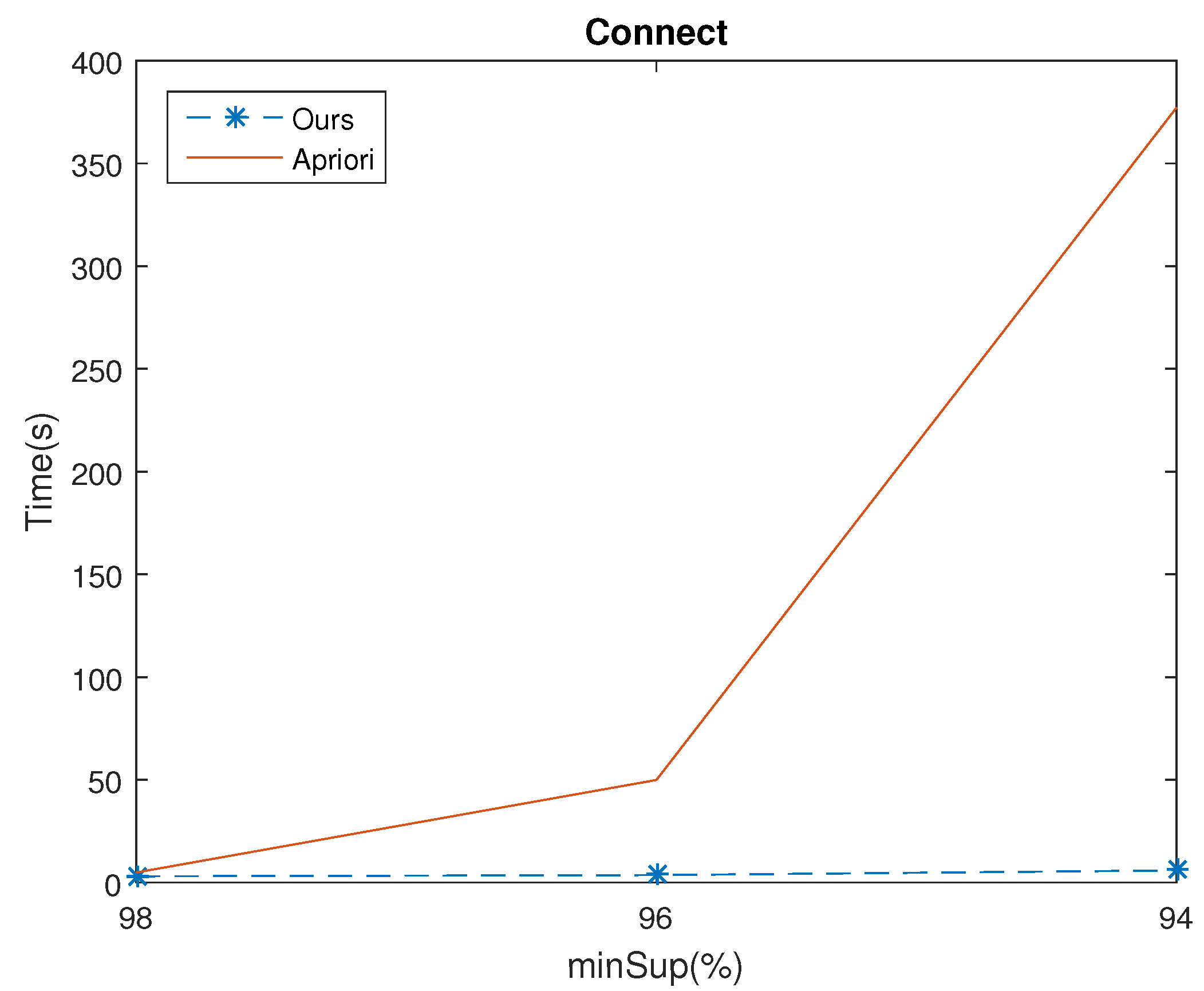
5.1. The Execution Time

Experiments were made to compare the execution time of the algorithms Apriori and ours.The minConf was set to 50%. The results of the four databases for various minSup values are shown in Figure 4, Figure 5, Figure 6 and Figure 7, which shows that the execution of our algorithm was faster than Apriori in all cases. For example, given m i n S u p = 75 % , for the Chess database, the mining time of Apriori and ours were 3035.53(s) and 507.33(s), respectively. The time ratio is 507.33 3035.53 × 100 % = 16.71 % . Besides, as the minSup is decreased, the time ratio is reduced also. For example, consider the Connect database with m i n S u p set at 98%, 96% and 94%, the speed up of the time ratio were 91.93%, 7.26% and 1.56%, respectively. The results demonstrate that the execution time of mining rules from ours was more efficient than Apriori.

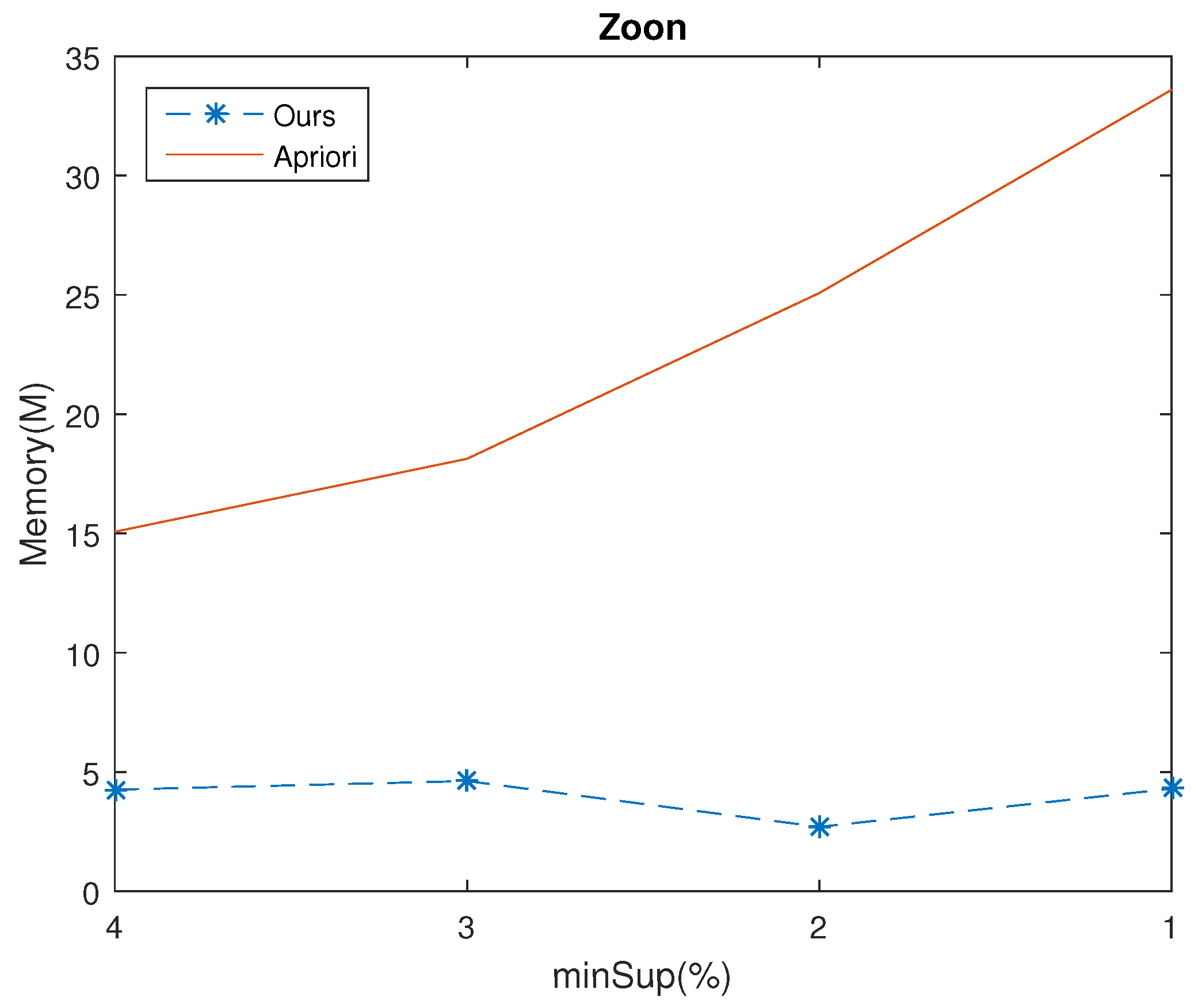
5.2. The Memory Usage

Experiments were made with the same databases and same parameters as the execution time experiments. The results show that the Apriori algorithm consumed more memory than ours in almost all cases, which are shown if Figure 8, Figure 9, Figure 10 and Figure 11. For example, given m i n S u p = 75 % , for Chess database, the memory usage of Apriori and ours were 672 (Mb) and 136.54 (Mb), respectively. The time ratio is 136.54 672 × 100 % = 20.32 % . Moreover, when we decrease the m i n S u p , the time ratio will reduce as well. For example, consider the Connect database with m i n S u p set at 98%, 96% and 94%, the speed up of the time ratio were 87.55%, 75.84% and 9.18%, respectively.

5.3. Numbers of Rules

We compare the numbers of association rules of Apriori with ours with the same databases and same parameters as the execution time experiments in Table 10. The results demonstrate that the numbers of ours is always smaller than those of Apriori. For example, given m i n S u p = 75 % , for Chess database, the number of rules of Apriori and ours were 2,336,556 and 253,836, respectively. The time ratio is 253836 2336556 × 100 % = 10.86 % . For our algorithm generating Min-Max association rules, the numbers of rules of ours is smaller than Apriori.
In this section, some examples are provided to show our method in association rules mining; transactional databases come from [62] and their characteristics are shown in Table 9. The Zoo database is initially used for classification of animals; in this paper, association rules among attributes of animals are considered, in which Min-Max association rules with confidence c = 1 and confidence c ( 0 , 1 ) will be shown, respectively. For mushroom database, connect-4 and chess, the topology, basis for the topology and equivalent classes with thresholds of support are obtained, and Min-Max association rules and generalized association rules are generated. Because the Reliable basis used to retrieve and reduce association rules in [63] is similar to our method, our results are compared with the method based on the Reliable basis limited in the number of Min-Max association rules and redundant rules.
Example 3.
In the Zoo database, there are 101 objects (animals) and 17 attributes (15 boolean, 2 numeric). Here, we discover association rules among 15 boolean attributes of animals, i.e., hair ( h a ), feathers ( f e ), eggs ( e g ), milk ( m i ), airborne ( a i ), aquatic ( a q ), predator ( p r ), toothed ( t o ), backbone ( b a ), breathes ( b r ), venomous ( v e ), fins ( f i ), tail ( t a ), domestic ( d o ) and catsize ( c a ).
According to Definition 1, 15 bases are generated (shown in Table A1 of Appendix A). Members of topology and equivalent classes with s u p p r ( ) are shown in Table A2 of Appendix A. Equivalent classes used to generate association rules with confidence c = 1 are shown in Table A3 of Appendix A. According to Table A3, 7 Min-Max association rules with s u p p r ( ) 0.4 and confidence c = 1 are generated (shown in Table A4 of Appendix A), in which m i b a b r (rule 4) is considered redundant of m i b a b r (rule 5) and m i b r b a (rule 6) due to { m i } { m i , b a } , { m i } { m i , b r } , { b r } { b a , b r } and { b a } { b a , b r } ; i.e., we use less conditions to achieve more results by m i b a b r with the same support and confidence. Furthermore, some Min-Max association rules generated in the quotient lattice of the topology with s u p p r ( ) 0.4 and confidence c ( 0 , 1 ) are shown in Table A5 of Appendix A, in which the Min-Max association rule b r b a and t a b a can be considered as a GAR of b r t a b a , respectively.
Example 4.
The mushroom database consists of a database with 8124 objects (mushrooms) and 22 nominally valued attributes. Here, we convert 22 nominally valued attributes as 126 boolean attributes and generate 111 bases. Change of bases with different s u p p r ( ) is shown in Figure A1 of Appendix A. Members of topology, equivalent classes and its generating time by using different bases are shown in Figure A2 of Appendix A.
Table A6 of Appendix A shows Min-Max association rules with s u p p r ( ) 0.8 and c = 1 . Compared with results in [63], rules 1–8 and 11 are same with [63], and rules 9, 10, 12 and 13 are new rules, in which rule 8 can be considered as a redundant rule of rules 9 and 10, rule 11 being a redundant rule of rules 12 and 13.
Table A7 of Appendix A show Min-Max association rules with s u p p r ( ) 0.8 and c [ 0.8 , 1 ) , in which rules 1–25 are also generated in [63]; rules 26-41 are new rules.
Table A8 of Appendix A shows comparative results, in which T R X means the number of all approximate rules in [63], Min-Max ( N , R t ) and Reliable ( N , R t ) means number and reduction ratio of Min-Max basis rules and reliable basis rules generated by Min-Max approximate basis, Min-Max exact basis, reliable approximate basis and reliable exact basis in [63]. T R means the number of all rules generated in the quotient lattice ( T ( R A ) / τ , , ) , N-Min-Max ( N , R t ) means the number and reduction ratio of Min-Max association rules generated in ( T ( R A ) / τ , , ) , the reduction ratio is calculated as R t = T R X N T R X or T R N T R . In Table A8, it can be noticed that the association rules used to obtain a reduction in the quotient lattice ( T ( R A ) / τ , , ) are less than in [63], such as for s u p p r ( ) 0.4 , 2528 association rules are used to obtain reduction. The lower s u p p r ( ) and confidence c is corresponding to more generated association rules and higher reduction ratio in the quotient lattice ( T ( R A ) / τ , , ) , such as for s u p p r ( ) 0.4 and confidence c 0.5 , 1825 rules are generated and the reduction ratio is 0.77.
Example 5.
In the connect-4 database, the number of reduction association rules with confidence c 0.5 and compared with in [63] are shown in Table A9 of Appendix A. For template A = { d 5 b , d 6 b , e 5 b , f 5 b , f 6 b } and rule ϕ a 6 b e 4 b f 5 b e 6 b f 6 b ,
L ( { d 5 b , d 6 b , e 5 b , f 5 b , f 6 b } ) = { d 5 b , d 6 b , f 5 b , f 6 b } , m i n [ { d 5 b , d 6 b , f 5 b , f 6 b } ] = { d 5 b , f 5 b } , L ( { a 6 b , e 4 b , f 5 b } ) = { a 6 b } , G ( { a 6 b , e 4 b , f 5 b } ) = { a 6 b , e 4 b , e 5 b , f 5 b } , L ( { e 6 b , f 6 b } ) = { e 6 b , f 6 b } , G ( { e 6 b , f 6 b } ) = { e 6 b , f 6 b } .
Accordingly, Table A10 shows the association rule of the template and generalized association rules in the connect-4 database.
In the chess database, the number of reduction association rules with confidence c 0.5 and compared with in [63] are shown in Table A11 of Appendix A. For template A = { m u l c h f , s k a c h f , w k n a 8 f } and rule ϕ q x m s q f s p c o p f w k n a 8 f b k o n 8 f h d c h k f ,
L ( { m u l c h f , s k a c h f , w k n a 8 f } ) = { m u l c h f , s k a c h f } , m i n [ { m u l c h f , s k a c h f } ] = { m u l c h f , s k a c h f } , L ( { q x m s q f , s p c o p f , w k n a 8 f } ) = { q x m s q f , s p c o p f } , G ( { q x m s q f , s p c o p f , w k n a 8 f } ) = { q x m s q f , s p c o p f , w k n a 8 f , s t l m t f } , L ( { b k o n 8 f , h d c h k f } ) = { b k o n 8 f , h d c h k f , r e s k d f } , G ( { b k o n 8 f , h d c h k f } ) = { b k o n 8 f , h d c h k f , r e s k d f , t h r s k f , s p c o p f } .
Accordingly, Table A12 shows the association rule of the template and generalized association rules in the chess database.

6. Conclusions

Association rules are often generated by frequent itemsets or closed itemsets from transactional databases. In order to obtain these itemsets, many methods have been proposed. In this article, for representing more general associative relations, which are among the items of transaction databases, the topology on itemset of a transactional database can been constructed. The topology on itemset includes frequent itemsets and closed itemsets. The topology on itemset includes frequent itemsets and closed itemsets, which has been proved. Most important of all, the basis of the topology can be used to generate the topology on the itemset, which deduced from the transactional database. Using the basis of the topology can efficiently avoid scanning databases many times in extracting association rules. The quotient lattice of the topology displays the hierarchical structures on all itemsets, because every closed itemset and its generators or minimal generators are limited in an element of the quotient lattice, valid Min-Max association rules can be easily generated in the element. Because the quotient lattice of the topology provides granular concepts to approximate any template of itemset, reductant association rules can be easily generated by granular concepts. The experiment demonstrates that association rules mining using topology for itemset is an efficient method.

Author Contributions

Conceptualization, Z.P.; methodology, Z.P. and B.L.; validation, C.Z. and F.H.; Writing—original draft, B.L.; Writing—review and editing, Z.P., formal analysis, Z.P. and B.L.; All authors have read and agreed to the published version of the manuscript.

Funding

This work has been partially supported by Talent introduction project of Xihua University (Z202104) and the Opening Project of Intelligent Policing Key Laboratory of Sichuan Province (Grant no. ZNJW2022KFMS004, ZNJW2022KFQN002, ZNJW2023KFQN007).

Data Availability Statement

Not applicable.

Conflicts of Interest

The authors declare no conflict of interest.

Appendix A

Table A1. Basis B A of Zoo database.
Attributes ha fe eg mi ai
Basis { h a , b r } { f e , e g , b a , b r , t a } { e g } { m i , b a , b r } { a i , b r }
Attributes a q p r t o b a b r
Basis { a q } { p r } { t o , b a } { b a } { b r }
Attributes v e f i t a d o c a
Basis { v e } { a q , t o , b a , f i } { t a } { d o } { c a }
Table A2. Members of topology and equivalent classes with s u p p r ( ) c .
c0 0.2 0.3 0.5
Members of topology4159985411
Equivalent classes237754411
Table A3. Equivalent classes used to generate association rules with s u p p r ( ) 0.3 and confidence c = 1 .
Equivalent Classes | [ ] | min [ ] P τ ( T )
[ { b a , b r , c a } ] 2 { { b r , c a } } { { b r , c a } }
[ { b a , b r , t a , c a } ] 2 { { b r , t a , c a } } { { b r , t a , c a } }
[ { b a , b r , t o } ] 1 { { b a , b r , t o } } { { b r , t o } }
[ { h a , b r } ] 1 { { h a , b r } } { { h a } }
[ { t o , b a , b r , t a } ] 1 { { t o , b a , b r , t a } } { { b r , t o , t a } }
[ { m i , t o , b a , b r } ] 1 { { m i , t o , b a , b r } } { { m i , t o } , { m i , t o , b a } ,
{ m i , t o , b r } }
[ { h a , m i , b a , b r } ] 2 { { h a , b a , b r } } { { h a , b a } , { h a , b a , b r } }
[ { m i , t o , b a , b r , t a } ] 1 { { m i , t o , b a , b r , t a } } { { m i , t o , t a } , { m i , t o , b a , t a } ,
{ m i , t o , b r , t a } }
[ { e g , b a , t a } ] 2 { { e g , t a } } { { e g , t a } }
[ { h a , m i , b a , b r , t a } ] 3 { { h a , b r , t a } } { { h a , t a } , { h a , b r , t a } }
[ { h a , m i , t o , b a , b r , t a } ] 2 { { h a , t o , b a , b r , t a } } { { h a , t o , t a } , { h a , t o , b a , b r , t a } ,
{ h a , t o , b r , t a } , { h a , t o , b a , t a } }
[ { p r , t o , b a , t a } ] 1 { { p r , t o , b a , t a } } { { p r , t o , t a } }
[ { t o , b a } ] 1 { { t o , b a } } { { t o } }
[ { p r , t o , b a } ] 1 { { p r , t o , b a } } { { p r , t o } }
[ { m i , b a , b r } ] 1 { { m i , b a , b r } } { { m i } , { m i , b a } , { m i , b r } }
[ { m i , b a , b r , t a } ] 1 { { m i , b a , b r , t a } } { { m i , t a } , { m i , b a , t a } ,
{ m i , b r , t a } }
[ { t o , b a , c a } ] 1 { { t o , b a , c a } } { { t o , c a } }
[ { m i , b a , b r , c a } ] 1 { { m i , b a , b r , c a } } { { m i , c a } , { m i , b a , c a } ,
{ m i , b r , c a } }
[ { m i , t o , b a , b r , c a } ] 2 { { t o , b a , b r , c a } } { { t o , b a , c a } , { t o , b a , b r , c a } }
[ { t o , b a , t a } ] 1 { { t o , b a , t a } } { { t o , t a } }
[ { h a , m i , t o , b a , b r } ] 2 { { h a , t o , b a , b r } } { { h a , t o } , { h a , t o , b a } ,
{ h a , t o , b r } , { h a , t o , b a , b r } }
[ { b a , t a , c a } ] 2 { { t a , c a } } { { t a , c a } }
Table A4. All Min-Max association rules with s u p p r ( ) 0.4 and c = 1 .
NumbersRule ϕ ( supp r ( ϕ ) , c )
1 b r t o b a ( 0.4653 , 1 )
2 h a b r ( 0.4257 , 1 )
3 t o b a ( 0.604 , 1 )
4 m i b a b r ( 0.4059 , 1 )
5 m i b a b r ( 0.4059 , 1 )
6 m i b r b a ( 0.4059 , 1 )
7 t o t a b a ( 0.5149 , 1 )
Table A5. Some Min-Max association rules with s u p p r ( ) 0.4 and 0.8 c < 1 .
NumbersRule ϕ ( supp r ( ϕ ) , c )
1 p r b a t a ( 0.4059 , 0.8723 )
2 p r t a b a ( 0.4059 , 0.9762 )
3 t a b r ( 0.604 , 0.8133 )
4 p r b a ( 0.4653 , 0.8393 )
5 c a b a ( 0.4257 , 0.9773 )
6 t o b a t a ( 0.5149 , 0.8525 )
7 t o b a t a ( 0.5149 , 0.8525 )
8 b a b r ( 0.6832 , 0.8313 )
9 b r b a ( 0.6832 , 0.8625 )
10 b a t a ( 0.7327 , 0.8916 )
11 t a b a ( 0.7327 , 0.9867 )
12 t a b a b r ( 0.5941 , 0.8 )
13 b a b r t a ( 0.5941 , 0.8696 )
14 b a t a b r ( 0.5941 , 0.8108 )
15 b r t a b a ( 0.5941 , 0.9836 )
Figure A1. Change of bases in the mushroom database corresponding to s u p p r ( ) .
Mathematics 11 00401 g0a1
Figure A2. Members of topology, equivalent classes and its generating time in the mushroom database corresponding to bases.
Mathematics 11 00401 g0a2
Table A6. All Min-Max association rules in the mushroom database with s u p p r ( ) 0.8 and c = 1 .
NRule ϕ ( supp r ( ϕ ) , c )
1 g i l l a t t a c h m e n t f v e i l t y p e p ( 0.9742 , 1 )
2 g i l l s p a c i n g c v e i l t y p e p ( 0.8385 , 1 )
3 v e i l c o l o r w v e i l t y p e p ( 0.9754 , 1 )
4 r i n g n u m b e r o v e i l t y p e p ( 0.9217 , 1 )
5 g i l l a t t a c h m e n t f v e i l c o l o r w v e i l t y p e p ( 0.9732 , 1 )
6 g i l l a t t a c h m e n t f r i n g n u m b e r o v e i l t y p e p ( 0.8981 , 1 )
7 g i l l s p a c i n g c v e i l c o l o r w v e i l t y p e p ( 0.8149 , 1 )
8 g i l l a t t a c h m e n t f g i l l s p a c i n g c v e i l c o l o r w v e i l t y p e p ( 0.8127 , 1 )
9 g i l l a t t a c h m e n t f g i l l s p a c i n g c v e i l t y p e p v e i l c o l o r w ( 0.8127 , 1 )
10 g i l l a t t a c h m e n t f g i l l s p a c i n g c v e i l c o l o r w v e i l t y p e p ( 0.8127 , 1 )
11 v e i l c o l o r w r i n g n u m b e r o g i l l a t t a c h m e n t f v e i l t y p e p ( 0.8971 , 1 )
12 g i l l a t t a c h m e n t f v e i l c o l o r w r i n g n u m b e r o v e i l t y p e p ( 0.8971 , 1 )
13 v e i l t y p e p v e i l c o l o r w r i n g n u m b e r o g i l l a t t a c h m e n t f ( 0.8971 , 1 )
Table A7. Min-Max association rules with s u p p r ( ) 0.8 and 0.8 c < 1 .
NumbersRule ϕ ( supp r ( ϕ ) , c )
1 v e i l t y p e p g i l l a t t a c h m e n t f ( 0.9742 , 0.9742 )
2 v e i l t y p e p g i l l s p a c i n g c ( 0.8385 , 0.8385 )
3 v e i l t y p e p v e i l c o l o r w ( 0.9754 , 0.9754 )
4 v e i l t y p e p r i n g n u m b e r o ( 0.9217 , 0.9217 )
5 v e i l t y p e p g i l l a t t a c h m e n t f v e i l c o l o r w ( 0.9732 , 0.9732 )
6 v e i l t y p e p g i l l a t t a c h m e n t f r i n g n u m b e r o ( 0.8981 , 0.8981 )
7 v e i l t y p e p g i l l s p a c i n g c v e i l c o l o r w ( 0.8149 , 0.8149 )
8 v e i l t y p e p g i l l a t t a c h m e n t f g i l l s p a c i n g c v e i l c o l o r w ( 0.8127 , 0.8127 )
9 v e i l t y p e p g i l l a t t a c h m e n t f v e i l c o l o r w r i n g n u m b e r o ( 0.8971 , 0.8971 )
10 g i l l a t t a c h m e n t f v e i l t y p e p v e i l c o l o r w ( 0.9732 , 0.999 )
11 g i l l a t t a c h m e n t f v e i l t y p e p r i n g n u m b e r o ( 0.8981 , 0.9219 )
12 g i l l a t t a c h m e n t f g i l l s p a c i n g c v e i l c o l o r w v e i l t y p e p ( 0.8127 , 0.8342 )
13 g i l l a t t a c h m e n t f v e i l c o l o r w r i n g n u m b e r o v e i l t y p e p ( 0.8971 , 0.9209 )
14 g i l l s p a c i n g c g i l l a t t a c h m e n t f v e i l c o l o r w v e i l t y p e p ( 0.8127 , 0.9692 )
15 g i l l s p a c i n g c v e i l c o l o r w v e i l t y p e p ( 0.8149 , 0.9718 )
16 v e i l c o l o r w g i l l s p a c i n g c v e i l t y p e p ( 0.8149 , 0.8354 )
17 v e i l c o l o r w g i l l a t t a c h m e n t f g i l l s p a c i n g c v e i l t y p e p ( 0.8127 , 0.8332 )
18 v e i l c o l o r w g i l l a t t a c h m e n t f v e i l t y p e p ( 0.9732 , 0.9977 )
19 v e i l c o l o r w g i l l a t t a c h m e n t f r i n g n u m b e r o v e i l t y p e p ( 0.8971 , 0.9197 )
20 r i n g n u m b e r o g i l l a t t a c h m e n t f v e i l t y p e p ( 0.8981 , 0.9744 )
21 r i n g n u m b e r o g i l l a t t a c h m e n t f v e i l c o l o r w v e i l t y p e p ( 0.8971 , 0.9733 )
22 g i l l a t t a c h m e n t f v e i l c o l o r w r i n g n u m b e r o v e i l t y p e p ( 0.8971 , 0.9218 )
23 g i l l a t t a c h m e n t f v e i l c o l o r w g i l l s p a c i n g c v e i l t y p e p ( 0.8127 , 0.8351 )
24 g i l l a t t a c h m e n t f r i n g n u m b e r o v e i l c o l o r w v e i l t y p e p ( 0.8971 , 0.9989 )
25 g i l l s p a c i n g c v e i l c o l o r w g i l l a t t a c h m e n t f v e i l t y p e p ( 0.8127 , 0.9973 )
26 g i l l a t t a c h m e n t f v e i l t y p e p v e i l c o l o r w r i n g n u m b e r o ( 0.8971 , 0.9209 )
27 g i l l a t t a c h m e n t f v e i l t y p e p r i n g n u m b e r o ( 0.8981 , 0.9219 )
28 v e i l t y p e p v e i l c o l o r w g i l l a t t a c h m e n t f r i n g n u m b e r o ( 0.8971 , 0.9197 )
29 v e i l t y p e p r i n g n u m b e r o g i l l a t t a c h m e n t f v e i l c o l o r w ( 0.8971 , 0.9733 )
30 v e i l t y p e p r i n g n u m b e r o g i l l a t t a c h m e n t f ( 0.8981 , 0.9744 )
31 g i l l a t t a c h m e n t f v e i l t y p e p v e i l c o l o r w r i n g n u m b e r o ( 0.8971 , 0.9218 )
32 g i l l a t t a c h m e n t f v e i l t y p e p r i n g n u m b e r o v e i l c o l o r w ( 0.8971 , 0.9989 )
33 g i l l a t t a c h m e n t f v e i l t y p e p g i l l s p a c i n g c v e i l c o l o r w ( 0.8127 , 0.8342 )
34 g i l l s p a c i n g c v e i l t y p e p g i l l a t t a c h m e n t f v e i l c o l o r w ( 0.8127 , 0.9692 )
35 v e i l t y p e p v e i l c o l o r w g i l l a t t a c h m e n t f g i l l s p a c i n g c ( 0.8127 , 0.8332 )
36 g i l l a t t a c h m e n t f v e i l t y p e p v e i l c o l o r w g i l l s p a c i n g c ( 0.8127 , 0.8351 )
37 g i l l s p a c i n g c v e i l t y p e p v e i l c o l o r w g i l l a t t a c h m e n t f ( 0.8127 , 0.9973 )
38 g i l l a t t a c h m e n t f v e i l t y p e p v e i l c o l o r w ( 0.9732 , 0.999 )
39 v e i l t y p e p v e i l c o l o r w g i l l a t t a c h m e n t f ( 0.9732 , 0.9977 )
40 g i l l s p a c i n g c v e i l t y p e p v e i l c o l o r w ( 0.8149 , 0.9718 )
41 v e i l t y p e p v e i l c o l o r w g i l l s p a c i n g c ( 0.8149 , 0.8354 )
Table A8. The number of approximate rules and reduction in the mushroom database with confidence c 0.5 .
supp r ( ) TRX Min-Max ( N , Rt )Reliable ( N , Rt ) TR N-Min-Max ( N , Rt )
0.42528(465, 0.82)(361, 0.86)1825(420, 0.77)
0.5835(175, 0.79)(135, 0.84)514(190, 0.63)
0.6228(59, 0.74)(52, 0.77)136(65, 0.52)
0.7161(39, 0.74)(34, 0.79)90(41, 0.54)
Average 0.770.82 0.62
Table A9. Number of approximate rules and reduction in the connect-4 database with confidence c 0.5 .
supp r ( ) TRX Min-Max ( N , Rt )Reliable ( N , Rt ) TR N-Min-Max ( N , Rt )
0.94199,560(49,407, 0.75)(10,220, 0.95)88,116( 7914 , 0.91 )
0.9577,206(24,794, 0.68)(5245, 0.93)39,768(4731, 0.88)
0.9626,856(11,452, 0.57)(2538, 0.91)16,356(2535, 0.85)
0.977895(4439, 0.44)(1214, 0.85)5690(1294, 0.77)
Average 0.610.91 0.85
Table A10. Templates, association rules and generalized association rules in the connect-4 database.
Template 1 A = { d 5 b , d 6 b , e 5 b , f 5 b , f 6 b } ( supp r ( A ) = 0.9573 )
ψ 1 d 5 b d 6 b f 5 b f 6 b e 5 b ( 0.9573 , 0.99 )
Reduction of ψ 1 d 5 b f 5 b e 5 b ( 0.9573 , 0.99 )
Rule 1 ϕ a 6 b e 4 b f 5 b e 6 b f 6 b ( 0.9502 , 0.9694 )
ϕ G A a 6 b e 6 b f 6 b ( 0.9502 , 0.9576 )
ϕ g a a 6 b e 4 b e 5 b f 5 b e 6 b f 6 b ( 0.9502 , 1 )
Table A11. The number of approximate rules and reduction in the chess database with confidence c 0.5 .
supp r ( ) TRX Min-Max ( N , Rt )Reliable ( N , Rt ) TR N-Min-Max ( N , Rt )
0.9010,614(8371, 0.21)(2483, 0.77)9230( 2034 , 0.78 )
0.915785(5050, 0.13)(1571, 0.73)5354(1357, 0.75)
0.932338(1948, 0.17)(688, 0.71)2110(648, 0.69)
0.95468(459, 0.02)(196, 0.58)466(195, 0.58)
Average 0.130.70 0.70
Table A12. Templates, association rules and generalized association rules in the chess database.
Template 1 A = { mulch f , skach f , wkna 8 f } ( supp r ( A ) = 0.9002 )
ψ 1 m u l c h f s k a c h f w k n a 8 f ( 0.9002 , 0.9492 )
Rule 1 ϕ q x m s q f s p c o p f w k n a 8 f b k o n 8 f h d c h k f r e s k d f t h r s k f ( 0.8326 , 0.9103 )
ϕ G A q x m s q f s p c o p f b k o n 8 f h d c h k f r e s k d f t h r s k f ( 0.8827 , 0.9107 )
ϕ G C q x m s q f s p c o p f w k n a 8 f b k o n 8 f h d c h k f r e s k d f ( 0.8698 , 0.9136 )
ϕ G A C q x m s q f s p c o p f b k o n 8 f h d c h k f r e s k d f ( 0.9215 , 0.9507 )
ϕ g a q x m s q f s p c o p f w k n a 8 f s t l m t f b k o n 8 f h d c h k f r e s k d f t h r s k f ( 0.8326 , 0.9103 )

References

  1. Agrawal, R.; Imieliński, T.; Swami, A. Mining Association Rules between Sets of Items in Large Databases. In Proceedings of the 1993 ACM SIGMOD International Conference on Management of Data, Washington, DC, USA, 25–28 May 1993; Association for Computing Machinery: New York, NY, USA, 1993; pp. 207–216. [Google Scholar]
  2. Agrawal, R.; Srikant, R. Fast Algorithms for Mining Association Rules in Large Databases. In Proceedings of the 20th International Conference on Very Large Data Bases, Santiago de Chile, Chile, 12–15 September 1994; Morgan Kaufmann Publishers Inc.: San Francisco, CA, USA, 1994; pp. 487–499. [Google Scholar]
  3. Thamer, M.B.; El-Sappagh, S.; El-Shishtawy, T. A Semantic Approach for Extracting Medical Association Rules. Int. J. Intell. Eng. Syst. 2020, 13, 280–292. [Google Scholar] [CrossRef]
  4. Razzak, M.I.; Imran, M.; Xu, G. Big data analytics for preventive medicine. Neural Comput. Appl. 2020, 32, 4417–4451. [Google Scholar] [CrossRef] [PubMed]
  5. Zhang, H.N.; Dwivedi, A.D. Precise Marketing Data Mining Method of E-Commerce Platform Based on Association Rules. Mob. Netw. Appl. 2022. [Google Scholar] [CrossRef]
  6. Reddy, R.V.; Venkateswara Rao, K.; Kameswara Rao, M.; Deepak Kumar, B.P. A Review on Stock Market Analysis Using Association Rule Mining. In Cybernetics, Cognition and Machine Learning Applications; Gunjan, V.K., Suganthan, P.N., Haase, J., Kumar, A., Eds.; Springer Nature Singapore: Singapore, 2023; pp. 171–183. [Google Scholar]
  7. Ahn, K.I.; Kim, J.Y. Efficient Mining of Frequent Itemsets and a Measure of Interest for Association Rule Mining. J. Inf. Knowl. Manag. 2004, 3, 245–257. [Google Scholar] [CrossRef]
  8. Brin, S.; Motwani, R.; Ullman, J.D.; Tsur, S. Dynamic itemset counting and implication rules for market basket data. In Proceedings of the 1997 ACM SIGMOD International Conference on Management of Data, Tucson, AZ, USA, 13–15 May 1997; ACM: New York, NY, USA, 1997; pp. 255–264. [Google Scholar]
  9. Geng, L.; Hamilton, H.J. Interestingness measures for data mining: A survey. ACM Comput. Surv. 2006, 38, 9. [Google Scholar] [CrossRef]
  10. Ghosh, A.; Nath, B. Multi-objective rule mining using genetic algorithms. Inf. Sci. 2004, 163, 123–133. [Google Scholar] [CrossRef]
  11. Silverstein, C.; Brin, S.; Motwani, R. Beyond market baskets: Generalizing association rules to dependence rules. Data Min. Knowl. Discov. 1998, 2, 39–68. [Google Scholar] [CrossRef]
  12. Baralis, E.; Cagliero, L.; Cerquitelli, T.; Garza, P. Generalized association rule mining with constraints. Inf. Sci. 2012, 194, 68–84. [Google Scholar] [CrossRef] [Green Version]
  13. Beiranvand, V.; Mobasher-Kashani, M.; Bakar, A.A. Multi-objective PSO algorithm for mining numerical association rules without a priori discretization. Expert Syst. Appl. 2014, 41, 4259–4273. [Google Scholar] [CrossRef]
  14. Guil, F.; Marín, R. A Theory of Evidence-based method for assessing frequent patterns. Expert Syst. Appl. 2013, 40, 3121–3127. [Google Scholar] [CrossRef]
  15. Guns, T.; Nijssen, S.; De Raedt, L. Itemset Mining: A Constraint Programming Perspective. Artif. Intell. 2011, 175, 1951–1983. [Google Scholar] [CrossRef] [Green Version]
  16. Ji, Y.; Ying, H.; Tran, J.; Dews, P.; Mansour, A.; Massanari, R.M. A Method for Mining Infrequent Causal Associations and Its Application in Finding Adverse Drug Reaction Signal Pairs. IEEE Trans. Knowl. Data Eng. 2013, 25, 721–733. [Google Scholar] [CrossRef] [Green Version]
  17. Kuo, R.J.; Chao, C.M.; Chiu, Y.T. Application of particle swarm optimization to association rule mining. Appl. Soft Comput. 2011, 11, 326–336. [Google Scholar] [CrossRef]
  18. Luna, J.M.; Romero, J.R.; Ventura, S. Grammar-based multi-objective algorithms for mining association rules. Data Knowl. Eng. 2013, 86, 19–37. [Google Scholar] [CrossRef]
  19. Rodríguez, D.M.; Rosete, A.; Alcalá-Fdez, J.; Herrera, F. QAR-CIP-NSGA-II: A new multi-objective evolutionary algorithm to mine quantitative association rules. Inf. Sci. 2014, 258, 1–28. [Google Scholar]
  20. Martínez-Ballesteros, M.; Martínez-Álvarez, F.; Lora, A.T.; Riquelme, J.C. Selecting the best measures to discover quantitative association rules. Neurocomputing 2014, 126, 3–14. [Google Scholar] [CrossRef]
  21. Pei, Z. Extracting association rules based on intuitionistic fuzzy special sets. In Proceedings of the FUZZ-IEEE, Hong Kong, China, 1–6 June 2008; pp. 873–878. [Google Scholar]
  22. Shaharanee, I.N.M.; Hadzic, F.; Dillon, T.S. Interestingness measures for association rules based on statistical validity. Knowl. Based Syst. 2011, 24, 386–392. [Google Scholar] [CrossRef]
  23. Kaushik, M.; Sharma, R.; Peious, S.A.; Shahin, M.; Yahia, S.B.; Draheim, D. A Systematic Assessment of Numerical Association Rule Mining Methods. SN Comput. Sci. 2021, 2, 348. [Google Scholar] [CrossRef]
  24. Kuo, R.J.; Gosumolo, M.; Zulvia, F.E. Multi-objective particle swarm optimization algorithm using adaptive archive grid for numerical association rule mining. Neural Comput. Appl. 2019, 31, 3559–3572. [Google Scholar] [CrossRef]
  25. Wang, H.B.; Gao, Y.J. Research on parallelization of Apriori algorithm in association rule mining. Procedia Comput. Sci. 2021, 183, 641–647. [Google Scholar] [CrossRef]
  26. Bazai, S.U.; Jang-Jaccard, J. In-Memory Data Anonymization Using Scalable and High Performance RDD Design. Electronics 2020, 9, 1732. [Google Scholar] [CrossRef]
  27. Bazai, S.U.; Jang-Jaccard, J.; Alavizadeh, H. A Novel Hybrid Approach for Multi-Dimensional Data Anonymization for Apache Spark. ACM Trans. Priv. Secur. 2021, 25, 1–25. [Google Scholar] [CrossRef]
  28. Bazai, S.U.; Jang-Jaccard, J.; Alavizadeh, H. Scalable, High-Performance, and Generalized Subtree Data Anonymization Approach for Apache Spark. Electronics 2021, 10, 589. [Google Scholar] [CrossRef]
  29. Calders, T.; Dexters, N.; Gillis, J.J.M.; Goethals, B. Mining frequent itemsets in a stream. Inf. Syst. 2014, 39, 233–255. [Google Scholar] [CrossRef]
  30. Han, J.; Cheng, H.; Xin, D.; Yan, X. Frequent pattern mining: Current status and future directions. Data Min. Knowl. Discov. 2007, 15, 55–86. [Google Scholar] [CrossRef] [Green Version]
  31. Pei, J.; Han, J.; Mao, R. CLOSET: An Efficient Algorithm for Mining Frequent Closed Itemsets. In Proceedings of the ACM SIGMOD Workshop on Research Issues in Data Mining and Knowledge Discovery, Dallas, TX, USA, 14 May 2000; pp. 21–30. [Google Scholar]
  32. Wang, J.; Han, J.; Pei, J. CLOSET+: Searching for the best strategies for mining frequent closed itemsets. In Proceedings of the KDD, Washington, DC, USA, 24–27 August 2003; Getoor, L., Senator, T.E., Domingos, P.M., Faloutsos, C., Eds.; ACM: New York, NY, USA, 2003; pp. 236–245. [Google Scholar]
  33. O’Sullivan, D.; Smyth, B.; Wilson, D.C.; McDonald, K.; Smeaton, A. Improving the Quality of the Personalized Electronic Program Guide. User Model. User-Adapt. Interact. 2004, 14, 5–36. [Google Scholar] [CrossRef] [Green Version]
  34. Kryszkiewicz, M.; Rybinski, H.; Gajek, M. Dataless Transitions Between Concise Representations of Frequent Patterns. J. Intell. Inf. Syst. 2004, 22, 41–70. [Google Scholar] [CrossRef]
  35. Pasquier, N.; Bastide, Y.; Taouil, R.; Lakhal, L. Efficient mining of association rules using closed itemset lattices. Inf. Syst. 1999, 24, 25–46. [Google Scholar] [CrossRef]
  36. Zaki, M.J. Scalable algorithms for association mining. IEEE Trans. Knowl. Data Eng. 2000, 12, 372–390. [Google Scholar] [CrossRef] [Green Version]
  37. Zaki, M.J.; Hsaio, C.J. Efficient Algorithms for Mining Closed Itemsets and Their Lattice Structure. IEEE Trans. Knowl. Data Eng. 2005, 17, 462–478. [Google Scholar] [CrossRef]
  38. Hashem, T.; Ahmed, C.F.; Samiullah, M.; Akther, S.; Jeong, B.S.; Jeon, S. An efficient approach for mining cross-level closed itemsets and minimal association rules using closed itemset lattices. Expert Syst. Appl. 2014, 41, 2914–2938. [Google Scholar] [CrossRef]
  39. Liu, H.; Liu, L.; Zhang, H. A fast pruning redundant rule method using Galois connection. Appl. Soft Comput. 2011, 11, 130–137. [Google Scholar] [CrossRef]
  40. Cagliero, L.; Cerquitelli, T.; Garza, P.; Grimaudo, L. Misleading Generalized Itemset discovery. Expert Syst. Appl. 2014, 41, 1400–1410. [Google Scholar] [CrossRef] [Green Version]
  41. Cagliero, L.; Garza, P. Itemset generalization with cardinality-based constraints. Inf. Sci. 2013, 244, 161–174. [Google Scholar] [CrossRef] [Green Version]
  42. Baralis, E.; Cagliero, L.; Cerquitelli, T.; D’Elia, V.; Garza, P. Expressive generalized itemsets. Inf. Sci. 2014, 278, 327–343. [Google Scholar] [CrossRef] [Green Version]
  43. Boulicaut, J.F.; Bykowski, A.; Rigotti, C. Free-sets: A condensed representation of boolean data for the approximation of frequency queries. Data Min. Knowl. Discov. 2003, 7, 5–22. [Google Scholar] [CrossRef]
  44. Bykowski, A.; Rigotti, C. DBC: A condensed representation of frequent patterns for efficient mining. Inf. Syst. 2003, 28, 949–977. [Google Scholar] [CrossRef] [Green Version]
  45. Chiang, D.A.; Wang, Y.F.; Wang, Y.H.; Chen, Z.Y.; Hsu, M.H. Mining disjunctive consequent association rules. Appl. Soft Comput. 2011, 11, 2129–2133. [Google Scholar] [CrossRef]
  46. Calders, T.; Goethals, B. Non-derivable itemset mining. Data Min. Knowl. Discov. 2007, 14, 171–206. [Google Scholar] [CrossRef] [Green Version]
  47. Li, H.; Chen, H. Mining non-derivable frequent itemsets over data stream. Data Knowl. Eng. 2009, 68, 481–498. [Google Scholar] [CrossRef]
  48. Hamrouni, T.; Yahia, S.B.; Nguifo, E.M. Sweeping the disjunctive search space towards mining new exact concise representations of frequent itemsets. Data Knowl. Eng. 2009, 68, 1091–1111. [Google Scholar] [CrossRef]
  49. Barrenechea, E.; Sola, H.B.; Campión, M.J.; Induráin, E.; Knoblauch, V. Topological interpretations of fuzzy subsets. A unified approach for fuzzy thresholding algorithms. Knowl. Based Syst. 2013, 54, 163–171. [Google Scholar] [CrossRef]
  50. Syau, Y.R.; Lin, E.B. Neighborhood systems and covering approximation spaces. Knowl. Based Syst. 2014, 66, 61–67. [Google Scholar] [CrossRef]
  51. Wang, S.; Liu, D. Knowledge representation and reasoning for qualitative spatial change. Knowl. Based Syst. 2012, 30, 161–171. [Google Scholar] [CrossRef]
  52. Pei, Z.; Ruan, D.; Meng, D.; Liu, Z. Formal concept analysis based on the topology for attributes of a formal context. Inf. Sci. 2013, 236, 66–82. [Google Scholar] [CrossRef]
  53. Zhang, Y.; Pei, Z.; Shi, P. Association rule mining based on topology for attributes of multi-valued information systems. Int. J. Innov. Comput. Inf. Control. Ijicic 2013, 9, 1679–1690. [Google Scholar]
  54. Ganter, B.; Wille, R. Formal Concept Analysis: Mathematical Foundations; Springer: Berlin/Heidelberg, Germany, 1999. [Google Scholar]
  55. Pawlak, Z.; Skowron, A. Rough sets and Boolean reasoning. Inf. Sci. 2007, 177, 41–73. [Google Scholar] [CrossRef] [Green Version]
  56. Qin, K.; Yang, J.; Pei, Z. Generalized rough sets based on reflexive and transitive relations. Inf. Sci. 2008, 178, 4138–4141. [Google Scholar] [CrossRef]
  57. Zhang, H.P.; Ouyang, Y.; Wang, Z. Note on “Generalized rough sets based on reflexive and transitive relations”. Inf. Sci. 2009, 179, 471–473. [Google Scholar] [CrossRef]
  58. Freund, M. On the notion of concept I. Artif. Intell. 2008, 172, 570–590. [Google Scholar] [CrossRef]
  59. Srikant, R.; Agrawal, R. Mining Generalized Association Rules. In Proceedings of the 21st International Conference on Very Large Databases, Zurich, Switzerland, 11–15 September 1995; pp. 407–419. [Google Scholar]
  60. Wu, C.M.; Huang, Y.F. Generalized association rule mining using an efficient data structure. Expert Syst. Appl. 2011, 38, 7277–7290. [Google Scholar] [CrossRef]
  61. Apriori Algorithm. Available online: http://www.mathworks.com/matlabcentral/fileexchange/42541-association-rules/ (accessed on 1 September 2022).
  62. UCI Machine Learning Repository. Available online: http://archive.ics.uci.edu/ml/ (accessed on 1 September 2022).
  63. Xu, Y.; Li, Y.; Shaw, G. Reliable representations for association rules. Data Knowl. Eng. 2011, 70, 555–575. [Google Scholar] [CrossRef]
Figure 1. The lattice of the topology T ( R A ) of Example 1.
Mathematics 11 00401 g001
Figure 2. The complete lattice ( T ( R A ) / τ , , ) of Example 1.
Mathematics 11 00401 g002
Figure 3. The complete lattice ( T ( R A ) / τ , , ) of Example 2.
Mathematics 11 00401 g003
Figure 4. Execution time of the two algorithms in Chess dataset for various minSup values.
Mathematics 11 00401 g004
Figure 5. Execution time of the two algorithms in Connect dataset for various minSup values.
Mathematics 11 00401 g005
Figure 6. Execution time of the two algorithms in Mushroom dataset for various minSup values.
Mathematics 11 00401 g006
Figure 7. Execution time of the two algorithms in Zoon dataset for various minSup values.
Mathematics 11 00401 g007
Figure 8. Memory usage of the two algorithms in Chess dataset for various minSup values.
Mathematics 11 00401 g008
Figure 9. Memory usage of the two algorithms in Connect dataset for various minSup values.
Mathematics 11 00401 g009
Figure 10. Memory usage of the two algorithms in Mushroom dataset for various minSup values.
Mathematics 11 00401 g010
Figure 11. Memory usage of the two algorithms in Zoon dataset for various minSup values.
Mathematics 11 00401 g011
Table 1. A transactional database A = ( U , A ) .
U A a 1 a 2 a 3 a 4 a 5
u 1 10001
u 2 10100
u 3 00101
u 4 01100
u 5 11111
u 6 00111
Table 2. The binary relation R A on A.
R A a 1 a 2 a 3 a 4 a 5
a 1 10000
a 2 01100
a 3 00100
a 4 00111
a 5 00001
Table 3. A transactional database A = ( U , A ) .
U A a 1 a 2 a 3 a 4 a 5
u 1 10101
u 2 00110
u 3 01001
u 4 10101
u 5 00110
u 6 11101
u 7 10111
u 8 11001
u 9 10001
u 10 00110
Table 4. A binary relation on A.
R A a 1 a 2 a 3 a 4 a 5
a 1 10001
a 2 01001
a 3 00100
a 4 00110
a 5 00001
Table 5. Closed itemset and minimal generators of each equivalent class.
Equivalent Class [ T ] min [ T ] min P τ ( T )
[ { a 1 , a 5 } ] { a 1 , a 5 } { a 1 , a 5 } { a 1 }
[ { a 2 , a 5 } ] { a 2 , a 5 } { a 2 , a 5 } { a 2 }
[ { a 3 , a 4 } ] { a 3 , a 4 } { a 3 , a 4 } { a 4 }
[ { a 1 , a 2 , a 5 } ] { a 1 , a 2 , a 5 } { a 1 , a 2 , a 5 } { a 1 , a 2 }
[ { a 3 , a 5 } ] { a 1 , a 3 , a 5 } { a 3 , a 5 } { a 3 , a 5 }
[ { a 2 , a 3 , a 5 } ] { a 1 , a 2 , a 3 , a 5 } { a 2 , a 3 , a 5 } { a 2 , a 3 }
[ { a 3 , a 4 , a 5 } ] { a 1 , a 3 , a 4 , a 5 } { a 3 , a 4 , a 5 } { a 4 , a 5 }
Table 6. Min-Max association rules with support s and confidence c = 1 .
Min-Max Association Rule(Support, Confidence)
a 1 a 5 ( 6 , 1 )
a 2 a 5 ( 3 , 1 )
a 4 a 3 ( 4 , 1 )
a 1 a 2 a 5 ( 2 , 1 )
a 3 a 5 a 1 ( 4 , 1 )
a 2 a 3 a 5 ( 1 , 1 )
a 2 a 3 a 5 a 1 ( 1 , 1 )
a 2 a 3 a 1 a 5 ( 1 , 1 )
a 4 a 5 a 3 ( 1 , 1 )
a 3 a 4 a 5 a 1 ( 1 , 1 )
a 4 a 5 a 1 a 3 ( 1 , 1 )
Table 7. Itemsets and their lower approximations of Example 2.
ItemsetsLower ApproximationsThe Set of Equivalent Classes
{ a 1 , a 3 } { a 3 } { [ { a 3 } ] }
{ a 3 , a 5 } { a 3 , a 5 } { [ { a 3 } ] , [ { a 5 } ] }
{ a 1 , a 3 , a 4 } { a 3 , a 4 } { [ { a 3 } ] , [ { a 3 , a 4 } ] }
Table 8. Min-Max association rules generated by the itemsets.
ItemsetsMin-Max Association Rules(Support, Confidence)
{ a 1 , a 3 } a 3 a 1 ( 4 , 4 7 )
{ a 3 , a 5 } a 3 a 5 ( 4 , 4 7 )
{ a 3 , a 5 } a 5 a 3 ( 4 , 4 7 )
{ a 1 , a 3 , a 4 } a 3 a 1 a 4 ( 1 , 1 7 )
{ a 1 , a 3 , a 4 } a 4 a 1 a 3 ( 1 , 1 4 )
Table 9. Dataset characteristics.
DatasetTransactionsOriginal AttributesAttributes after Conversion
Zoo1011715
Mushroom812423126
Connect-467,55743129
Chess319636108
Table 10. Number of rules of Apriori and Ours.
Dataset minSup ( % ) Number of Rules
AprioriOurs
Chess95472700
9010,7429482
8595,48243,116
80552,564111,768
752,336,556253,836
Mushroom501146172
452704291
405006483
3514,107903
3045,145903
Connect981544380
9627,3401480
94201,9283848
Zoon429,2888136
335,2048826
248,5785110
164,8688174
Disclaimer/Publisher’s Note: The statements, opinions and data contained in all publications are solely those of the individual author(s) and contributor(s) and not of MDPI and/or the editor(s). MDPI and/or the editor(s) disclaim responsibility for any injury to people or property resulting from any ideas, methods, instructions or products referred to in the content.

