Feature Map Regularized CycleGAN for Domain Transfer

Abstract

CycleGAN domain transfer architectures use cycle consistency loss mechanisms to enforce the bijectivity of highly underconstrained domain transfer mapping. In this paper, in order to further constrain the mapping problem and reinforce the cycle consistency between two domains, we also introduce a novel regularization method based on the alignment of feature maps probability distributions. This type of optimization constraint, expressed via an additional loss function, allows for further reducing the size of the regions that are mapped from the source domain into the same image in the target domain, which leads to mapping closer to the bijective and thus better performance. By selecting feature maps of the network layers with the same depth d in the encoder of the direct generative adversarial networks (GANs), and the decoder of the inverse GAN, it is possible to describe their d-dimensional probability distributions and, through novel regularization term, enforce similarity between representations of the same image in both domains during the mapping cycle. We introduce several ground distances between Gaussian distributions of the corresponding feature maps used in the regularization. In the experiments conducted on several real datasets, we achieved better performance in the unsupervised image transfer task in comparison to the baseline CycleGAN, and obtained results that were much closer to the fully supervised pix2pix method for all used datasets. The PSNR measure of the proposed method was, on average, 4.7% closer to the results of the pix2pix method in comparison to the baseline CycleGAN over all datasets. This also held for SSIM, where the described percentage was 8.3% on average over all datasets.

1. Introduction

Analogous to automatic language translation, the task of image-to-image domain translation is to transfer images from one domain to another, preserving at the same time the content from the original images. For example, photographs could be transferred to drawings or presented in the style of a famous painter, winter landscapes could be transformed into summer landscapes and vice versa, while the training itself could be supervised using pairs of one-to-one matched image representations from both domains, or unsupervised, using any two images from the source and target domain. Image transfer found its applications in various image processing tasks, computer graphics, computer vision, and many other areas, including semantic image synthesis [1,2,3,4,5], style transfer [6,7,8], image imprinting [9,10,11], and image super-resolution [12,13].

Concerning the supervised training scenario, image-to-image domain translation is mostly conducted using conditional generative adversarial networks (cGANs) [14], a supervised extension of the concept of generative adversarial networks (GANs) [15], which uses paired image datasets. The concept was originally proposed in [16] in the form of the so-called pix2pix algorithm, and further expanded in [17,18,19]. GANs have found numerous applications related to generating synthetic datasets, including complex image data such as multispectral images, as recently presented in [20]. Regardless of its efficiency, there are still some drawbacks, such as the inability to capture the structural relationships of complex scenes through a single translation network, e.g., in the case when two domains have drastically different views. More importantly, for most real-world domain transfer tasks, the number of paired training images is seriously restricted [21,22]. In [5], the authors used the CycleGAN network architecture consisting of two GANs, the first transferring from the source to the target domain, and the second transferring from the target to the source domain. The problem arose as the introduced transforms, i.e., mappings were highly underconstrained. It was resolved by introducing the cycle consistency loss, which constrains the training so that the mapping does not deviate from bijectivity to a greater extent. Such a constraint is very efficient in preserving semantic information and important content of data, not just images in the task of image-to-image domain translation [5], but also other data types in emotion style transfer [23], speech enhancement [24], voice conversion [25], image dehazing without paired image data [26], and various other tasks. The cycle consistency loss used in [5] enforced the bijectivity of the network mappings by introducing a penalty term into the cost function. Besides the usual unpaired CycleGAN architectures, a hybrid approach in the form of conditional CycleGAN was also presented recently in [27].

The term was given in the form of $l_1$ norm between the input image from the source, i.e., the “left” domain and the cycling image obtained by performing the composition of “left” to “right”, i.e., the target domain, with “right” to “left” mappings, and vice versa, averaged by the overall number of image samples.

The idea and thus the novelty behind this paper are the following:

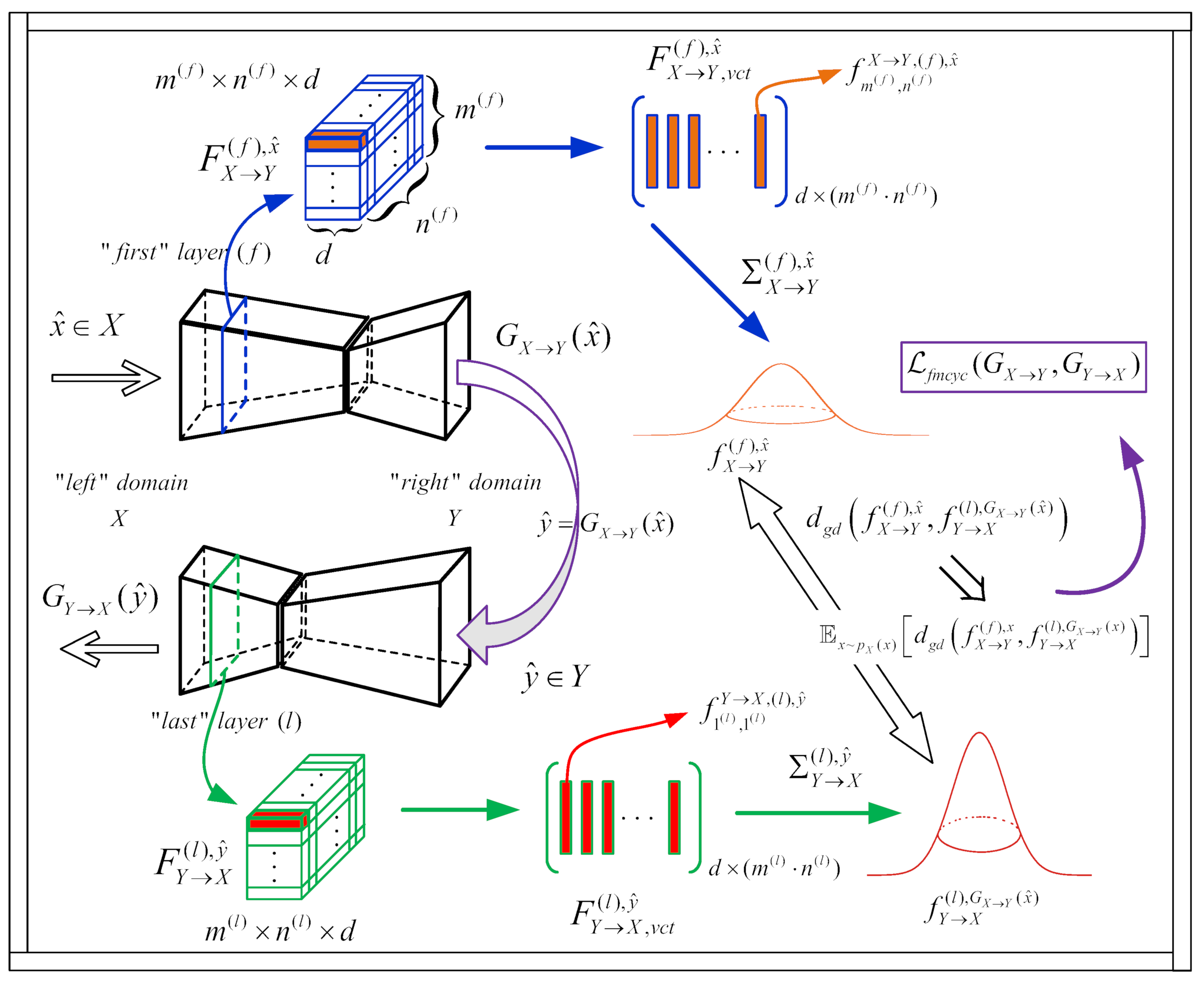
• We impose an additional feature-map-based cycle consistency loss to the overall optimization objective by introducing similarity measures between probability density functions (PDFs) modelling the statistics of the feature maps corresponding to “left” to “right” and “right” to “left” convolutional neural network (CNN) GANs where feature maps belong to the same level, i.e., a layer in the CycleGAN network architecture. Thus, an additional cycle consistency type of penalty term in the form of a similarity measure between PDFs is introduced in the overall cost function. Namely, we compare the distributions built upon the feature maps in the first network layer of the “left” to “right” GAN generator (its encoder) and the feature maps in the last network layer of the “right” to “left” GAN generator (its decoder) in order to achieve the transfer between the two domains that would be closer to bijective mapping.
• We apply various statistics-based measures and Riemannian-metrics, i.e., geodesic ground distance measures between the mentioned PDFs, where we impose the assumption that the PDFs are of the Gaussian type. As there exists an embedding of Gaussians into the cone, i.e., the Riemannian manifold of the symmetric positive definite (SPD) matrices, it is possible to apply various ground distance measures between the mentioned SPD matrices. A chosen ground distance is then minimized as the term in the overall network cost function during the training phase.

This novel approach is called Feature Map Regularized CycleGAN (FMR CycleGAN). As the number of feature maps, i.e., the depth of the corresponding convolutional network layers in the direct and the inverse GAN generators, is the same, we used this exact dimension, denoted by d, as the one over which the feature vector observations are defined, and the parameters of the two multivariate Gaussian distributions from the proposed penalty function are estimated for each input sample in the training set. Such feature-map-based cycle consistency showed good performance throughout the experiments over different datasets.

The paper is organized as follows. In Section 2, Section 2.2 the architecture of the baseline CycleGAN network is described and explained. In Section 2.3, various ground distances between Gaussians modelling the statistics of the feature maps, i.e., the corresponding SPD matrices, are presented and subsequently utilized as an additional term in the overall cost function. The proposed FMR CycleGAN method is introduced in Section 2.4. In Section 3, experimental results are presented, proving that the proposed approach obtained significantly better results than those of the baseline CycleGAN method presented in [5] and even close to the fully supervised pix2pix method proposed in [16], on three different datasets. In Section 4, conclusions are drawn. In order to ease the exposition, in the Appendix A we introduce the list of symbols used in the text.

2. Materials and Methods

In this section, we describe the baseline CycleGAN and the proposed FMR CycleGAN method, and introduce various ground distances between d-dimensional Gaussians, i.e., SPD matrices examined in the paper. Before that, we also discuss some related works.

2.1. Related Works

In general, image-to-image domain translation tasks can be solved in an unsupervised or supervised manner, and in a semisupervised setting. This implies that, in the case of supervised methods such as pix2pix [16], DRPAN [17], SPADE [1], or ASAPNet [28], generative models are trained on a set of paired images from the “left” and “right” domains, i.e., paired images corresponding to the same content. On the other hand, unsupervised methods such as UNIT [29], CycleGAN [5], DiscoGAN [30], CoGAN [31], or SimGAN [32] learn the corresponding mappings by using sets of unpaired images from the two domains. In the CycleGAN framework, this is accomplished by employing a cycle-consistency objective that enforces closeness between the original image and the one obtained by a full cycle of mappings, from the “left” to the “right” domain and backwards.

The proposed method belongs to a class of unsupervised approaches that expand the original CycleGAN framework, which was modified and applied in various tasks described in [23,24,25,26]. The general problem of unsupervised approaches is that the learned models usually implement one-to-many mappings, which is less favorable in terms of domain translation in comparison to the supervised methods that are from the beginning constrained to learn one-to-one mappings. Recently, there have been some efforts to improve the performance of unsupervised methods by introducing the regularization of the adversarial objective, which is the part of the overall cost function in all CycleGAN-based learning frameworks. Thus, in [33], the authors proposed a novel regularization of the adversarial objective that penalized the sensitivity of the discriminator in the CycleGAN. This is achieved through stochastic data augmentation function that perturbs the images, but in a semantics-preserving manner. In contrast to this type of regularization that targets the adversarial objective and aims at improving the stability of discriminators (by forcing them to be invariant to randomly augmented data), the proposed approach introduces novel-feature-based regularization in the cycle-consistency objective, which results in an alignment in the feature space. A detailed overview of image-to-image translation methods was also recently given in [34].

2.2. Baseline CycleGAN Approach

Generative adversarial networks were proposed in [15] as a ground-breaking method of nonparametrically learning the true data distribution. In an adversarial framework, the discriminator network D is trying to discriminate between the samples generated by the generator network G and the ground truth observations. The generative neural network model implementing the generator G describes the true data distribution, and during the model training, it learns to confuse the discriminator. Thus, the discriminator and the generator models compete in order to reach the Nash equilibrium expressed by the mini–max loss of the training procedure, where the optimization problem is given by:

$$\underset{G}{min}\underset{D}{max}{\mathbb{E}}_{x\sim p\left(x\right)}ln\left[D\left(x\right)\right]+{\mathbb{E}}_{z\sim p\left(z\right)}ln\left[(1-D\left(G\left(z\right)\right))\right],$$

(1)

where $p\left(x\right)$ represents the true data distribution, while the latent variable z is sampled by the distribution $p\left(z\right)$. ${\mathbb{E}}_{x\sim p\left(x\right)}$ corresponds to mathematical expectation with respect to $p\left(x\right)$.

CycleGAN was designed to capture the special characteristics of one image collection and establish how these could be translated into another image collection in the absence of any supervisor, i.e., paired training samples, as using those is not just difficult, but also expensive in terms of the labelling effort that has to be employed.

Let us denote the source, i.e., the “left” domain by X and the target, i.e., the “right” domain by Y. In [5], the authors proposed invoking the cycle consistency loss to the overall loss function using two domain translators in the form of GANs in domainwise mutually opposite directions, $L:X\to Y$ and $M:Y\to X$, thereby encouraging both mappings F and G to be “close” to bijection, i.e., $M\left(L\right(x\left)\right)\approx x$, and $L\left(M\right(y\left)\right)\approx y$, and thus compensating the lack of paired data samples. If the mappings L and M are implemented by the generator networks $G_{X\to Y}$ and $G_{Y\to X}$, respectively, and the discriminators in the domains X and Y are implemented by neural networks $D_X$ and $D_Y$, respectively, we obtain the following adversarial objectives:

$$\begin{array}{ccc}\hfill & & {\mathcal{L}}_{adv}(G_{X\to Y},D_Y)={\mathbb{E}}_{y\sim p_Y\left(y\right)}[ln{D}_Y\left(y\right)]+{\mathbb{E}}_{x\sim p_X\left(x\right)}[ln(1-D_Y\left(G_{X\to Y}\left(x\right)\right))],\hfill \end{array}$$

(2)

$$\begin{array}{ccc}& & {\mathcal{L}}_{adv}(G_{Y\to X},D_X)={\mathbb{E}}_{x\sim p_X\left(x\right)}[ln{D}_X\left(x\right)]+{\mathbb{E}}_{y\sim p_Y\left(y\right)}[ln(1-D_X\left(G_{Y\to X}\left(y\right)\right))],\hfill \end{array}$$

(3)

and the cycle-consistency objective:

$$\begin{array}{ccc}\hfill {\mathcal{L}}_{cyc}(G_{X\to Y},G_{Y\to X})& =& {\mathbb{E}}_{x\sim p_X\left(x\right)}[\parallel G_{Y\to X}\left(G_{X\to Y}\left(x\right)\right)-x\parallel ]\hfill \end{array}$$

(4)

$$\begin{array}{ccc}& \hspace{1em}\hspace{1em}\hspace{1em}\hspace{1em}\hspace{1em}\hspace{1em}\hspace{1em}\hspace{1em}+& {\mathbb{E}}_{y\sim p_Y\left(y\right)}[\parallel G_{X\to Y}\left(G_{Y\to X}\left(y\right)\right)-y\parallel ],\hfill \end{array}$$

(5)

making the full objective be given by:

$$\begin{array}{ccc}\hfill {\mathcal{L}}_{CycleGAN}(G_{X\to Y},G_{Y\to X},D_X,D_Y)& =& {\mathcal{L}}_{adv}(G_{X\to Y},D_Y)+{\mathcal{L}}_{adv}(G_{Y\to X},D_X)\hfill \\ & +& {\lambda }_{cyc}{\mathcal{L}}_{cyc}(G_{X\to Y},G_{Y\to X}),\hfill \end{array}$$

(6)

where ${\lambda }_{cyc}$ controls the relative importance of the objectives.

2.3. Ground Distances

In this subsection, we present the ground distances between d-dimensional Gaussians: $f=\mathcal{N}(x;{\mu }_1,{\Sigma }_1)$ and $g=\mathcal{N}(x;{\mu }_2,{\Sigma }_2)$, i.e., SPD matrices, used in our experiments. Symbol $\mathcal{N}$ denotes Gaussian or normal multivariate distribution. Besides Euclidean-based distances, $l_2$-based distance is given by:

$$d_{l_2}(f,g)=\parallel {\Sigma }_1-{\Sigma }_2{\parallel }_F+\eta {\parallel {\mu }_1-{\mu }_2\parallel }_{l_2},$$

(7)

and robust $l_1$-based distance given by:

$$d_{l_1}(f,g)=\parallel {\Sigma }_1-{\Sigma }_2{\parallel }_{l_1}+\eta {\parallel {\mu }_1-{\mu }_2\parallel }_{l_1},$$

(8)

where ${\parallel ·\parallel }_F$ is the Frobenius norm defined for $A=\left[a_{ij}\right]\in {\mathbb{R}}^{m\times n}$ as ${\parallel A\parallel }_F=\sqrt{{\sum }_{i=1}^m{\sum }_{j=1}^n{\left|a_{ij}\right|}^2}$, ${\parallel ·\parallel }_{l_2}$ is $l_2$ and ${\parallel ·\parallel }_{l_1}$ is $l_1$ (robust) norm in ${\mathbb{R}}^d$, and $\eta >0$, the ground distances between d-dimensional Gaussians could also be divided into two categories: statistics-based distances and Riemannian manifold-based distances.

Statistics-based distances employ information similarity measures between Gaussians considered to be as PDFs. There are various statistics-based distances used in the literature, such as the Chernoff divergence given in [35], Bhattacharyya divergence described in [36], or the Kullback–Leibler (KL) divergence presented in [37]). The latter is often adopted to compute the similarity between two probability density functions, especially in the case of two Gaussian densities. KL divergence between two arbitrary PDFs f and g defined in ${\mathbb{R}}^d$ is given by $d_{KL}(f,g)={\int }_{{\mathbb{R}}^d}f\left(x\right)ln\frac{f\left(x\right)}{g\left(x\right)}dx$. Moreover, there is a closed-form expression for the KL divergence between two arbitrary Gaussians $f=\mathcal{N}(x;{\mu }_1,{\Sigma }_1)$ and $g=\mathcal{N}(x;{\mu }_2,{\Sigma }_2)$, given by:

$$d_{KL}(f,g)=\frac{1}{2}{({\mu }_1-{\mu }_2)}^T{\Sigma }_1^{-1}({\mu }_1-{\mu }_2)+\frac{1}{2}\left({\Sigma }_1^{-1}{\Sigma }_2\right)-d$$

(9)

In our work, we used the symmetrized version of the KL divergence given by:

$$d_{K{L}_{sym}}(f,g)=\frac{1}{2}(d_{KL}(f,g)+d_{KL}(g,f)).$$

(10)

Concerning the Riemannian manifold-based distances, the shape of the Gaussian (SoG) transforms one Gaussian into a positive definite affine matrix through a positive definite lower triangular affine transformation (see [38]). Unlike SoG, the Gaussian embedding (GE) distance identifies each d-dimensional multivariate Gaussian as the SPD matrix P, defined in the following way by expression (please see [39,40]):

$$f=\mathcal{N}(x;\mu ,\Sigma )\mapsto P={|\Sigma |}^{-\frac{1}{d+1}}\left[\begin{array}{cc}\Sigma +\mu {\mu }^T& \mu \\ {\mu }^T& 1\end{array}\right],$$

(11)

where $|·|$ denotes the matrix determinant. $\mathcal{N}(x;\mu ,\Sigma )$ denotes the d-dimensional multivariate Gaussian distribution with centroid $\mu$ and covariance $\Sigma$. The cone of SPD matrices forms the Riemannian manifold, where the log-Euclidean (LE) metric is imposed as the metric tensor [41], forming the efficient geodesic distance invariant to similarity transformation given by:

$$d_{le}(P_1,P_2)={\parallel ln\left(P_1\right)-ln\left(P_2\right)\parallel }_F,$$

(12)

for $P_1,P_2\in {\mathrm{Sym}}_{++}\left(d\right)$, where ${\mathrm{Sym}}_{++}\left(d\right)$ is the cone of SPD matrices of format $d\times d$. Improved Gaussian embedding (IGE) distance introduces an additional balance parameter, $\nu >0$, by inserting $\nu \mu$ instead of $\mu$ into (11), thus balancing between $\mu$ and $\Sigma$. The product of Lie groups (PLG) [40] could be used as an alternative to (12), and for embeddings $P_i$, $i\in \{1,2\}$ defined by (11), the PLG is defined as:

$$d_{plg}(P_1,P_2)=\theta {\left[{({\mu }_1-{\mu }_2)}^T\left({\Sigma }_1^{-1}+{\Sigma }_2^{-1}\right)({\mu }_1-{\mu }_2)\right]}^{1/2}+(1-\theta ){\parallel ln\left(P_1\right)-ln\left(P_2\right)\parallel }_F,$$

(13)

for mixing coefficient $\theta \in (0,1)$. As shown in (13), the first term measures a type of Mahalanobis distance between the centroids of multivariate distributions, while the second term corresponds to the geodesic distance between the particular covariances using the log-Euclidean distance.

2.4. Proposed FMR CycleGAN Approach

The standard cycle consistency objective term in (6), and given by (4) enforces the bijectivity of mappings $G_{X\to Y}$ and $G_{Y\to X}$ by imposing the robust $l_1$ loss between the original and transformed images obtained through composition with previously mentioned mappings. Regularization is performed in the sense that there are no large regions in the “left” and “right” domains that are mapped to the same image by mappings $G_{X\to Y}$ and $G_{Y\to X}$, respectively. We propose adding an additional cycle consistency objective term that performs a similar regularization of the overall objective, but this time in the feature map domain.

Let us denote the first and the last feature map tensors in the GAN network generator $G_{X\to Y}$ by $F_{X\to Y}^{\left(f\right),\widehat{x}}\in {\mathbb{R}}^{m^{\left(f\right)}\times n^{\left(f\right)}\times d}$ and $F_{X\to Y}^{\left(l\right),\widehat{x}}\in {\mathbb{R}}^{m^{\left(l\right)}\times n^{\left(l\right)}\times d}$, respectively, when the sample $\widehat{x}\in X$ is propagated. Let us also denote the first and the last feature map tensors in the GAN network generator $G_{Y\to X}$ by $F_{Y\to X}^{\left(f\right),\widehat{y}}\in {\mathbb{R}}^{m^{\left(f\right)}\times n^{\left(f\right)}\times d}$ and $F_{Y\to X}^{\left(l\right),\widehat{y}}\in {\mathbb{R}}^{m^{\left(l\right)}\times n^{\left(l\right)}\times d}$ respectively, when the sample $\widehat{y}\in Y$ is propagated. In the general case of different neural network architectures, the value of $m^{\left(f\right)}$ in $G_{X\to Y}$ can be different from $m^{\left(l\right)}$ in $G_{Y\to X}$, and similar also holds for $n^{\left(f\right)}$ and $n^{\left(l\right)}$.

However, we impose the condition that the third dimension of these feature map tensors, denoted by d, is the same, as illustrated in Figure 1. We also assumed that the same network architecture was used for mappings $G_{X\to Y}$ and $G_{Y\to X}$ (in our particular case, we used a generator network architecture proposed in [42]).

We can reformat $F_{X\to Y}^{\left(q\right),\widehat{x}}$ and $F_{Y\to X}^{\left(q\right),\widehat{y}}$, $q\in \{f,l\}$ into matrices:

$$F_{X\to Y,vct}^{\left(q\right),\widehat{x}}=\left[f_{1,1}^{X\to Y\left(q\right),\widehat{x}}|f_{1,2}^{X\to Y,\left(q\right),\widehat{x}},\dots |f_{m^{\left(q\right)},n^{\left(q\right)}}^{X\to Y,\left(q\right),\widehat{x}}\right],$$

(14)

and

$$F_{Y\to X,vct}^{\left(q\right),\widehat{y}}=\left[f_{1,1}^{Y\to X,\left(q\right),\widehat{y}}|f_{1,2}^{Y\to X,\left(q\right),\widehat{y}},\dots |f_{m^{\left(q\right)},n^{\left(q\right)}}^{Y\to X,\left(q\right),\widehat{y}}\right],$$

(15)

where $f_{i,j}^{X\to Y,\left(q\right),\widehat{x}},f_{i,j}^{Y\to X,\left(q\right),\widehat{y}}\in {\mathbb{R}}^d$, $i\in \{1,\dots ,m^{\left(q\right)}\}$, $j\in \{1,\dots ,n^{\left(q\right)}\}$, $q\in \{f,l\}$.

Feature map tensors in the “first” and the “last” layers of the CycleGAN generators, and the process of obtaining corresponding matrices with d-dimensional feature vectors (observations) by their reshaping are described in Figure 1.

Thus, we obtain the maximum likelihood (ML) estimates ${\Sigma }_{X\to Y}^{\left(q\right),\widehat{x}}$ and ${\Sigma }_{Y\to X}^{\left(q\right),\widehat{y}}$, $q\in \{f,l\}$ of covariances of unknown PDFs that render the d-dimensional observations (values in the feature map tensors), i.e., ML estimates are based on the columns of matrices $F_{X\to Y,vct}^{\left(q\right),\widehat{x}}$ and $F_{Y\to X,vct}^{\left(q\right),\widehat{y}}$, $q\in \{f,l\}$, respectively, by imposing the assumption that the underlying PDFs are d-dimensional multivariate Gaussians. This is also shown in Figure 1, where it is graphically indicated that the shape of Gaussians depends on the content of the corresponding feature map tensors. Therefore, it holds that:

$$\begin{array}{ccc}\hfill & & {\Sigma }_{X\to Y}^{\left(q\right),\widehat{x}}=\frac{1}{m^{\left(q\right)}{n}^{\left(q\right)}}\sum _{i=1}^{m^{\left(q\right)}}\sum _{j=1}^{n^{\left(q\right)}}(f_{i,j}^{X\to Y,\left(q\right),\widehat{x}}-{\mu }_{X\to Y}^{\left(q\right),\widehat{x}}){(f_{i,j}^{X\to Y,\left(q\right),\widehat{x}}-{\mu }_{X\to Y}^{\left(q\right),\widehat{x}})}^T,\hfill \\ & & {\Sigma }_{Y\to X}^{\left(q\right),\widehat{y}}=\frac{1}{m^{\left(q\right)}{n}^{\left(q\right)}}\sum _{i=1}^{m^{\left(q\right)}}\sum _{j=1}^{n^{\left(q\right)}}(f_{i,j}^{Y\to X,\left(q\right),\widehat{y}}-{\mu }_{Y\to X}^{\left(q\right),\widehat{y}}){(f_{i,j}^{Y\to X,\left(q\right),\widehat{y}}-{\mu }_{Y\to X}^{\left(q\right),\widehat{y}})}^T,\hfill \end{array}$$

(16)

where

$$\begin{array}{ccc}\hfill & & {\mu }_{X\to Y}^{\left(q\right),\widehat{x}}=\frac{1}{m^{\left(q\right)}{n}^{\left(q\right)}}\sum _{i=1}^{m^{\left(q\right)}}\sum _{j=1}^{n^{\left(q\right)}}{f}_{i,j}^{X\to Y,\left(q\right),\widehat{x}},\hfill \\ & & {\mu }_{Y\to X}^{\left(q\right),\widehat{y}}=\frac{1}{m^{\left(q\right)}{n}^{\left(q\right)}}\sum _{i=1}^{m^{\left(q\right)}}\sum _{j=1}^{n^{\left(q\right)}}{f}_{i,j}^{Y\to X,\left(q\right),\widehat{y}},\hfill \end{array}$$

(17)

are obtained by propagating samples $\widehat{x}\in X$ and $\widehat{y}\in Y$, and $q\in \{f,l\}$. On the basis of the previous assumptions, we can now form the novel feature-map-based cycle consistency objective term as follows:

$$\begin{array}{ccc}\hfill & & {\mathcal{L}}_{fmcyc}(G_{X\to Y},G_{Y\to X})=E_{x\sim p_X\left(x\right)}\left[d_{gd}\left(f_{X\to Y}^{\left(f\right),x},f_{Y\to X}^{\left(l\right),G_{X\to Y}\left(x\right)}\right)\right]\hfill \\ & & +E_{y\sim p_Y\left(y\right)}\left[d_{gd}\left(f_{Y\to X}^{\left(f\right),y},f_{X\to Y}^{\left(l\right),G_{Y\to X}\left(y\right)},\right)\right]\hfill \end{array}$$

(18)

where $d_{gd}$ denotes some of the ground distances described in Section 2.3, making the full FMR CycleGAN objective function be given by:

$$\begin{array}{ccc}\hfill & & {\mathcal{L}}_{FMRCycleGAN}(G_{X\to Y},G_{Y\to X},D_X,D_Y)={\mathcal{L}}_{adv}(G_{X\to Y},D_Y)+{\mathcal{L}}_{adv}(G_{Y\to X},D_X)\hfill \\ & & +{\lambda }_{cyc}{\mathcal{L}}_{cyc}(G_{X\to Y},G_{Y\to X})+{\lambda }_{fmcyc}{\mathcal{L}}_{fmcyc}(G_{X\to Y},G_{Y\to X}),\hfill \end{array}$$

(19)

where ${\lambda }_{fmcyc}>0$ is fixed. Concerning ground distances $d_{gd}$, for the purpose of experiments, we used Euclidian distance $d_{l_1}$ given by (8), statistics, i.e., information-based distance $d_{KLsym}$, given by (10), and Riemannian manifold-based distance $d_{le}$, given by (12), together with the embedding described in (13).

3. Results and Discussion

In this section, we deliver the network architecture details and experimental results obtained by comparing the proposed novel FMR CycleGAN method with the baseline CycleGAN proposed in [5] and the pix2pix method proposed in [16]. The results are presented for several image datasets in the task of image-to-image translation, showing the efficiency of the proposed domain transformation method in comparison to the above-mentioned baselines.

For our experiments, we used the following datasets that were evaluated over the corresponding image domain translation tasks: the CityScapes dataset within the semantic photo2labels task [16,43], containing 2975 training image pairs and an additional 500 image pairs in the test set (gtFine_trainvaltest.zip and leftImg8bit_trainvaltest.zip were used in our experiments); the CMP Facade dataset within the architectural photo2labels task [16,44] containing 400 training image pairs and an additional 106 image pairs used for evaluation purposes; the Google Maps dataset within the aerial2map task [16] containing 1096 training image pairs and an additional 1098 image pairs aimed for validation purposes. Images from the last training set were selected among Google Maps images taken across the Manhattan region of the city of New York (satellite images were used in pairs with the corresponding Google Maps images).

3.1. Network Architecture

Concerning the GAN architecture, for the main neural network architecture of the GANs corresponding to generator networks $G_{X\to Y}$ and $G_{Y\to X}$, the original CycleGAN architecture proposed in [5] was adopted. This architecture, which was also utilized in [24], contains one stride-1 and two stride-2 convolutions that are followed by several residual blocks and 2 fractionally strided convolutions with stride $1/2$. The network consists of 6 blocks for $128\times 128$ images and 9 blocks for $256\times 256$ pixels and images with higher-resolution. Instance normalization reported in [5,42,45] was also utilized. Since GANs are adversarial models, the discriminator networks consist of $70\times 70$ PatchGAN network, previously reported in [16,46]. Concerning the training details, the L2 loss approach invoked in [5] was employed instead of the negative log-likelihood loss approach in (1), as it was documented to be more stable. Moreover, as in [5], we used the history of 50 generated images to calculate the average score. We also used ${\lambda }_{cyc}={\lambda }_{fmcyc}=10$ for all our experiments. The size of the set of minibatches was always kept at $m=50$. The networks were initialized using a random distribution $\mathcal{N}(0,0.02)$. All of the networks were trained using the learning rate of $\eta =0.0002$, which was kept constant during the first 100 training epochs and then linearly decayed to zero during the subsequent 100 epochs.

3.2. Evaluation Metrics

In the domain of image-to-image translation tasks, the evaluation of the quality of synthesized images is still an open research problem. To evaluate the quality of synthesized images, we used standard and objective reference-based measures such as peak signal-to-noise ratio (PSNR) and the more advanced structural similarity index (SSIM). As an energy-preserving measure based on the mean squared error between the ideal and the obtained solutions (image), the PSNR score expressed in decibels is sometimes overly optimistic. Therefore, the SSIM index is also used as the objective-perception-based model, which considers image degradation as perceived change in structural information. It also incorporates important perceptual phenomena, including both luminance masking and contrast masking terms. Thus, the SSIM measure is much more appropriate for measuring image degradation than PSNR is. The PSNR was evaluated as follows:

$$PSNR=20log\frac{MA{X}_I}{\sqrt{MSE}},$$

(20)

where $MA{X}_I$ is the maximal possible pixel value of the ground truth images, while $MSE$ is the squared Euclidean norm between the generated and ground truth images. The SSIM measure between images generated by the considered GAN algorithms and the ground truth images was calculated on various image frames using the following formula:

$$SSIM(x,y)=\frac{(2{\mu }_x{\mu }_y+c_1)(2{\sigma }_{xy}+c_2)}{({\mu }_x^2+{\mu }_y^2+c_1)({\sigma }_x^2+{\sigma }_y^2+c_2)},$$

(21)

where ${\mu }_x$ and ${\mu }_y$ are pixel sample means along dimensions x and y of the image, ${\sigma }_x^2$ and ${\sigma }_y^2$ are corresponding variances and $c_1$ and $c_2$ are constants set as reported in [47].

In addition to the above, classical reference-based image quality assessment (IQA) metrics, fully convolutional neural network (FCN) scores proposed in [48] were also employed. The FCN scores measure the performance of semantic segmentation algorithms by computing different quantities corresponding to segmentation accuracy at the level of individual pixels. Thus, semantic segmentation maps generated by some image domain translation algorithms can be directly compared against the ground truth semantic labels provided in the utilized dataset of labeled images. Similar to [48], the same types of measures assessing the quality of pixel labeling were used in all experiments. However, instead of obtaining semantic labels by FCN image segmentation model proposed in [48], the results of presented experiments were obtained by image domain translation using designed supervised and unsupervised generative models.

FCN measures or scores include pixel accuracy, defined as ${\sum }_i{n}_{ii}/{\sum }_i{t}_i$, mean accuracy, evaluated as $(1/n_{cl}){\sum }_i{n}_{ii}/t_i$, and the mean region intersection over union (IoU) accuracy, evaluated as $(1/n_{cl}){\sum }_i{n}_{ii}/\left(t_i+{\sum }_j{n}_{ji}-n_{ii}\right)$. $n_{ij}$ is the number of pixels of class i predicted to belong to class j, $n_{cl}$ is the number of classes, and $t_i={\sum }_j{n}_{ij}$ is the total number of pixels belonging to the class i. These standard measures provided precise comparison of the proposed algorithm against the baselines.

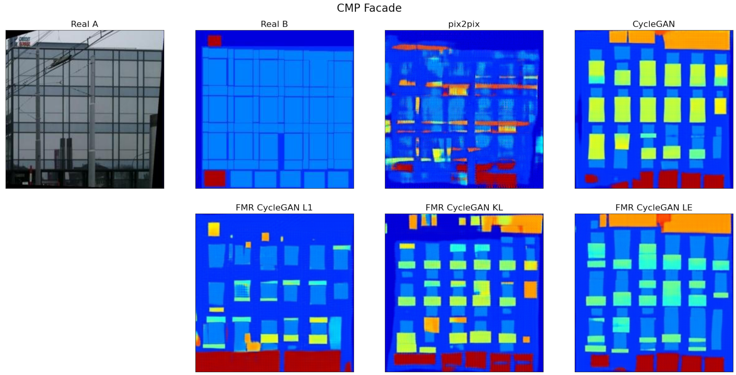
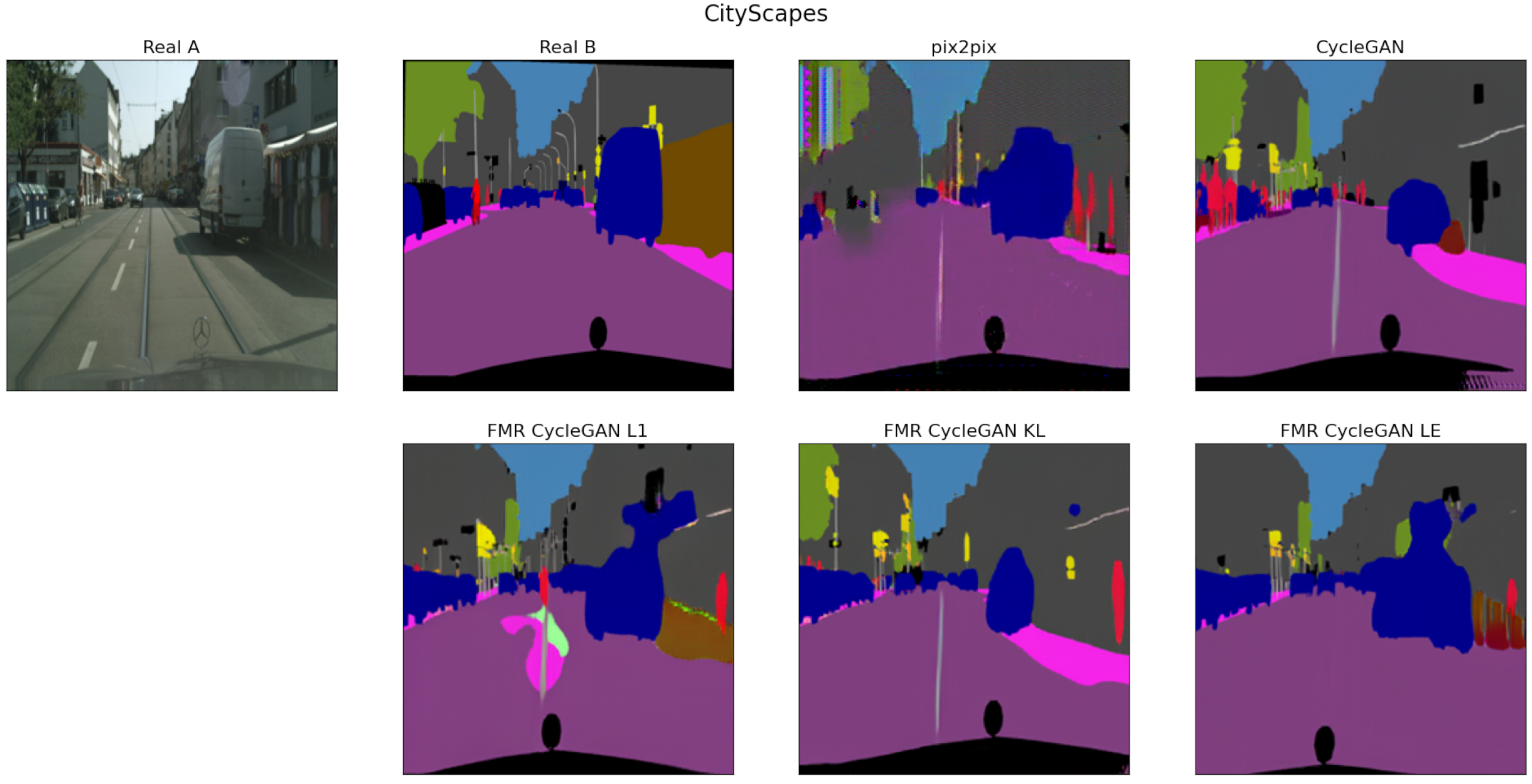
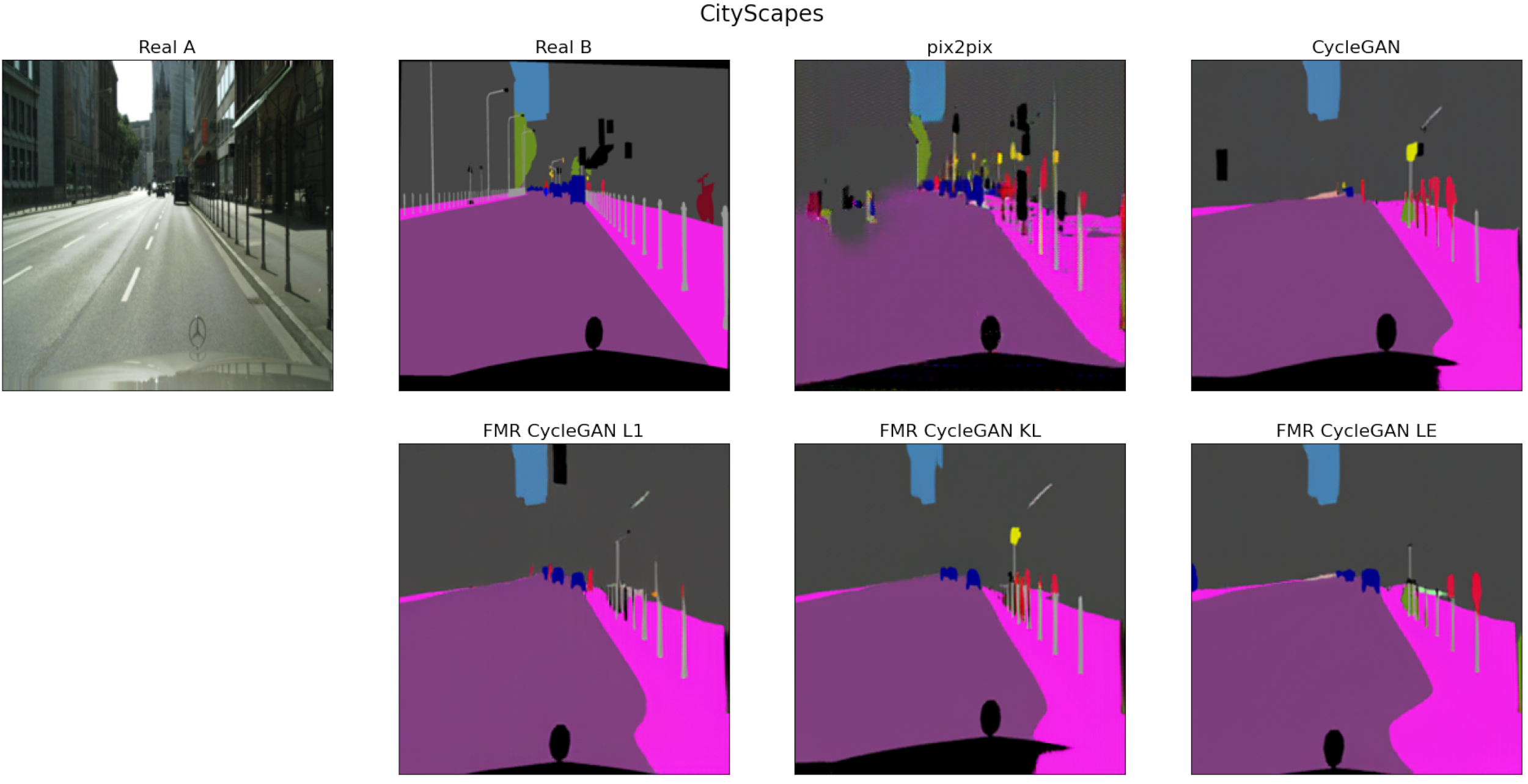
3.3. Experimental Results and Comparisons

The experimental results of PSNR and SSIM measures between the generated and the ground truth images are presented in

Table 1. PSNR measures for the proposed FMR CycleGAN in comparison to the baseline methods for different used ground distances (the best unsupervised results are highlighted in bold and gray).

Dataset/Task	pix2pix	CycleGAN	FMR CycleGAN
			${\mathit{d}}_{{\mathit{l}}_{\mathbf{1}}}$	${\mathit{d}}_{{\mathit{KL}}_{\mathit{sym}}}$	${\mathit{d}}_{\mathit{el}}$
Google Maps	30.01	30.24	31.15	30.85	30.32
CMP Fasade	14.25	10.98	10.81	11.45	11.37
CityScapes	19.51	17.12	17.89	18.86	17.34

and

Table 2. SSIM measures for the proposed FMR CycleGAN in comparison to the baseline methods for different used ground distances (the best unsupervised results are highlighted in bold and gray).

Dataset/Task	pix2pix	CycleGAN	FMR CycleGAN
			${\mathit{d}}_{{\mathit{l}}_{\mathbf{1}}}$	${\mathit{d}}_{{\mathit{KL}}_{\mathit{sym}}}$	${\mathit{d}}_{\mathit{el}}$
Google Maps	0.69	0.73	0.76	0.74	0.73
CMP Fasade	0.42	0.27	0.31	0.29	0.28
CityScapes	0.59	0.54	0.58	0.65	0.56

, and provide a direct comparison between the proposed FMR CycleGAN method, and the baseline pix2pix and CycleGAN methods. The comparisons were conducted for all three datasets. For ground distance in FMR CycleGAN, three different similarity measures were examined: $d_{l_1}$ given by (8) (it performed better than $d_{l_2}$), $d_{K{L}_{sym}}$ given by (10) and (9) and $d_{le}$ given by (12), using Embedding (11), where $\nu$ was set heuristically to $0.4$ for all experiments. pix2pix, as a fully supervised method, obtained the best results in almost all experiments in comparison to all considered unsupervised methods, as it was expected. Nevertheless, the proposed FMR CycleGAN obtained the best results (for various used ground distances) among the considered unsupervised methods. The best performing algorithms among the unsupervised methods are highlighted in bold and gray.

The proposed FMR CycleGAN method achieved better results on average regarding both PSNR and SSIM measures for all used ground distances and over all experiments in comparison to the baseline CycleGAN method. Moreover, these results were close to those of the fully supervised pix2pix method. In

Table 3. FCN scores of the proposed FMR CycleGAN against the baseline unsupervised and supervised methods, for different ground distances utilized in feature map regularization. The results correspond to semantic photo2label domain translation task performed on the CityScapes dataset (the best unsupervised results are highlighted in bold and gray).

Image-to-Image		FCN Score Type
Translation Method		Pixel Acc.	Mean Acc.	Mean IoU
supervised:	pix2pix	0.71	0.25	0.18
unsupervised:	CycleGAN	0.52	0.17	0.11
	CoGAN	0.40	0.10	0.06
	SimGAN	0.20	0.10	0.04
FMR CycleGAN	${\mathit{d}}_{{\mathit{l}}_{\mathbf{1}}}$	0.59	0.22	0.15
	${\mathit{d}}_{\mathit{K}{\mathit{L}}_{\mathit{s}\mathit{y}\mathit{m}}}$	0.56	0.20	0.17
	${\mathit{d}}_{\mathit{e}\mathit{l}}$	0.15	0.17	0.13

, the FCN accuracy scores of the proposed FMR CycleGAN are compared with those of the baseline supervised and unsupervised methods in the semantic photo2labels task, which was performed on the CityScapes dataset. The same conclusion could be drawn as in the case of results in Table 1 and Table 2. The proposed FMR CycleGAN method obtained better results in comparison to the baseline CycleGAN method, and those of the CoGAN and SimGAN methods, for all unsupervised experiments and ground distances used; however, the FMR CycleGAN was outperformed by the fully supervised pix2pix method, as it was expected. Thus, the FMR component ${\mathcal{L}}_{fmcyc}$, defined by (18) and invoked within the overall cost function, significantly contributed to the overall performance of the proposed domain translation method for all ground distances within the proposed FMR framework.

When it comes to an overall quantitative comparison of average PSNRs of the proposed method against the average PSNRs of the baseline CycleGAN, the proposed method was on average 4.7% closer to the results of the pix2pix method as compared to the baseline CycleGAN (when relative PSNR differences between the unsupervised method and pix2pix are averaged over all datasets). This also holds for SSIM, where the described percentage in favor of the proposed method against the baseline CycleGAN was 8.3%, i.e., SSIM also indicated that FMR CycleGAN was on average closer to the pix2pix solution over all datasets. Besides the quantitative results in Table 1, Table 2 and Table 3, the performance of the proposed FMR CycleGAN (with various ground distances) was also assessed against the baseline CycleGAN (as unsupervised) and pix2pix (as supervised) method by visual comparisons presented in Figure 2, Figure 3, Figure 4, Figure 5, Figure 6 and Figure 7. Thus, for a pair of images from the “left” and “right” domains, i.e., images denoted as “Real A” and “Real B” in Figure 2, Figure 3, Figure 4, Figure 5, Figure 6 and Figure 7, respectively, image outputs generated by the “left” to “right” mappings of the compared algorithms are shown next to each other for different image domain translation tasks (datasets). These tasks were the following: the Google Maps aerial2map task in Figure 2 and Figure 3, the CMP Facades photo2labels task in Figure 4 and Figure 5, and the CityScapes photo2labels task in Figure 6 and Figure 7. Images that were used as the ground truth for obtaining previously described quantitative performance measures (“Real B” images in Figure 2, Figure 3, Figure 4, Figure 5, Figure 6 and Figure 7) also served as the ground truth in order to objectively assess the visual appearance of all methods. A visual comparison shows that the proposed regularization feature map term in the unsupervised FMR CycleGAN resulted in better performance (image outputs visually closer to “Real B”), when FMR CycleGAN was directly compared against the unsupervised CycleGAN method, and in an improvement over the CycleGAN when the two unsupervised methods were compared with the performance of the supervised pix2pix method for all presented tasks and datasets (Google Maps, CityScapes, and Facade). This can be explained by the fact that the proposed additional alignment between the feature maps of the direct and the inverse mappings enhanced the overall cycle consistency. Thus, the proposed FMR CycleGAN method obtained visually and structurally more accurate results than those of the baseline.

4. Conclusions

In this paper, we proposed adding a novel feature map regularization term in the overall loss function of the original CycleGAN network, forcing the bijectivity of the mappings even further, and thus obtaining the Feature Map Regularized (FMR) CycleGAN network for image domain translation. The proposed FMR term is a type of cycle consistency loss defined in the space of probability distributions of the d-dimensional column vectors of the feature map tensors. In order to measure the loss, we introduced several ground distances, both information-based and Riemannian manifold-based, between Gaussians representing PDFs of observations belonging to feature maps corresponding to direct and reverse GANs in the CycleGAN architecture. In the experiments presented on several real datasets, we obtained better results of image domain translation using the proposed method in comparison to the baseline CycleGAN method, and much closer to the fully supervised pix2pix method on all datasets. The overall performance improvement was only in the framework of the CycleGAN approach and the cycle consistency loss, which could be a limiting factor in the context of general domain transfer methods. In terms of implementation, the introduced geodesic and information distances are computationally complex, which renders the model training phase much more computationally demanding. However, no computational overhead was introduced in the model deployment phase.

References

1. Park, T.; Liu, M.-Y.; Wang, T.-C.; Zhu, J.-Y. Semantic image synthesis with spatially-adaptive normalization. In Proceedings of the IEEE/CVF Conference on Computer Vision and Pattern Recognition, Long Beach, CA, USA, 15–20 June 2019; pp. 2337–2346. [Google Scholar]
2. Zhu, P.; Abdal, R.; Qin, Y.; Wonka, P. Sean: Image synthesis with semantic region-adaptive normalization. In Proceedings of the IEEE/CVF Conference on Computer Vision and Pattern Recognition, Seattle, WA, USA, 14–19 June 2020; pp. 5104–5113. [Google Scholar]
3. Lee, C.-H.; Liu, Z.; Wu, L.; Luo, P. Maskgan: Towards diverse and interactive facial image manipulation. In Proceedings of the IEEE/CVF Conference on Computer Vision and Pattern Recognition, Seattle, WA, USA, 14–19 June 2020; pp. 5549–5558. [Google Scholar]
4. Tang, H.; Xu, D.; Yan, Y.; Torr, P.H.; Sebe, N. Local class-specific and global image-level generative adversarial networks for semantic-guided scene generation. In Proceedings of the IEEE/CVF Conference on Computer Vision and Pattern Recognition, Seattle, WA, USA, 14–19 June 2020; pp. 7870–7879. [Google Scholar]
5. Zhu, J.-Y.; Park, T.; Isola, P.; Efros, A.A. Unpaired image-to-image translation using cycle-consistent adversarial networks. In Proceedings of the IEEE International Conference on Computer Vision, Venice, Italy, 22–29 October 2017; pp. 2223–2232. [Google Scholar]
6. Yi, Z.; Zhang, H.; Tan, P.; Gong, M. Dualgan: Unsupervised dual learning for image-to-image translation. In Proceedings of the IEEE International Conference on Computer Vision, Venice, Italy, 22–29 October 2017; pp. 2849–2857. [Google Scholar]
7. Alami Mejjati, Y.; Richardt, C.; Tompkin, J.; Cosker, D.; Kim, K.I. Unsupervised attention-guided image-to-image translation. In Proceedings of the 32nd Conference on Neural Information Processing Systems (NeurIPS 2018), Montreal, QC, Canada, 3–8 December 2018; Volume 32, pp. 3693–3703. [Google Scholar]
8. Tomei, M.; Cornia, M.; Baraldi, L.; Cucchiara, R. Art2real: Unfolding the reality of artworks via semantically-aware image-to-image translation. In Proceedings of the IEEE/CVF Conference on Computer Vision and Pattern Recognition, Long Beach, CA, USA, 15–20 June 2019; pp. 5849–5859. [Google Scholar]
9. Song, Y.; Yang, C.; Lin, Z.; Liu, X.; Huang, Q.; Li, H.; Kuo, C.-C.J. Contextual-based image inpainting: Infer, match, and translate. In Proceedings of the European Conference on Computer Vision (ECCV), Munich, Germany, 8–14 September 2018; pp. 3–19. [Google Scholar]
10. Liu, M.-Y.; Huang, X.; Mallya, A.; Karras, T.; Aila, T.; Lehtinen, J.; Kautz, J. Few-Shot Unsupervised Image-to-Image Translation. In Proceedings of the IEEE/CVF International Conference on Computer Vision, Seoul, Republic of Korea, 27 October–2 November 2019; pp. 10551–10560. [Google Scholar]
11. Zhao, L.; Mo, Q.; Lin, S.; Wang, Z.; Zuo, Z.; Chen, H.; Xing, W.; Lu, D. UCTGAN: Diverse image inpainting based on unsupervised cross-space translation. In Proceedings of the IEEE/CVF Conference on Computer Vision and Pattern Recognition, Seattle, WA, USA, 14–19 June 2020; pp. 5741–5750. [Google Scholar]
12. Yuan, Y.; Liu, S.; Zhang, J.; Zhang, Y.; Dong, C.; Lin, L. Unsupervised image super-resolution using cycle-in-cycle generative adversarial networks. In Proceedings of the IEEE Conference on Computer Vision and Pattern Recognition Workshops, Salt Lake City, UT, USA, 18–22 June 2018; pp. 701–710. [Google Scholar]
13. Zhang, Y.; Liu, S.; Dong, C.; Zhang, X.; Yuan, Y. Multiple cycle-in-cycle generative adversarial networks for unsupervised image super-resolution. IEEE Trans. Image Process. 2019, 29, 1101–1112. [Google Scholar] [CrossRef] [PubMed]
14. Mirza, M.; Osindero, S. Conditional generative adversarial nets. arXiv 2014, arXiv:1411.1784. [Google Scholar]
15. Goodfellow, I.; Pouget-Abadie, J.; Mirza, M.; Xu, B.; Warde-Farley, D.; Ozair, S.; Courville, A.; Bengio, Y. Generative adversarial networks. Commun. ACM 2020, 63, 139–144. [Google Scholar] [CrossRef]
16. Isola, P.; Zhu, J.-Y.; Zhou, T.; Efros, A.A. Image-to-image translation with conditional adversarial networks. In Proceedings of the IEEE Conference on Computer Vision and Pattern Recognition, Honolulu, HI, USA, 21–26 July 2017; pp. 1125–1134. [Google Scholar]
17. Wang, C.; Zheng, H.; Yu, Z.; Zheng, Z.; Gu, Z.; Zheng, B. Discriminative region proposal adversarial networks for high-quality image-to-image translation. In Proceedings of the European Conference on Computer Vision, Munich, Germany, 8–14 September 2018; pp. 770–785. [Google Scholar]
18. Wang, T.-C.; Liu, M.-Y.; Zhu, J.-Y.; Tao, A.; Kautz, J.; Catanzaro, B. High-resolution image synthesis and semantic manipulation with conditional GANs. In Proceedings of the IEEE Conference on Computer Vision and Pattern Recognition, Salt Lake City, UT, USA, 18–22 June 2018; pp. 8798–8807. [Google Scholar]
19. AlBahar, B.; Huang, J.-B. Guided image-to-image translation with bi-directional feature transformation. In Proceedings of the IEEE/CVF International Conference on Computer Vision, Seoul, South Korea, 27 October–2 November 2019; pp. 9016–9025. [Google Scholar]
20. Abady, L.; Dimitri, G.; Barni, M. Detection and localization of GAN manipulated multi-spectral satellite images. In Proceedings of the ESANN, Bruges, Belgium, 5–7 October 2022; pp. 339–344. [Google Scholar]
21. Hosseini-Asl, E.; Zhou, Y.; Xiong, C.; Socher, R. Robust domain adaptation by augmented cyclic adversarial learning. In Proceedings of the 31st International Conference on Neural Information Processing Systems—Interpretability and Robustness for Audio, Speech and Language Workshop, Montreal, QC, Canada, 3–8 December 2018; pp. 3–8. [Google Scholar]
22. Qi, C.; Chen, J.; Xu, G.; Xu, Z.; Lukasiewicz, T.; Liu, Y. SAG-GAN: Semi-supervised attention-guided GANs for data augmentation on medical images. arXiv 2020, arXiv:2011.07534. [Google Scholar]
23. Bao, F.; Neumann, M.; Vu, N.T. CycleGAN-based emotion style transfer as data augmentation for speech emotion recognition. In Proceedings of the INTERSPEECH, Graz, Austria, 15–19 September 2019; pp. 2828–2832. [Google Scholar]
24. Meng, Z.; Li, J.; Gong, Y. Cycle-consistent speech enhancement. arXiv 2018, arXiv:1809.02253. [Google Scholar]
25. Kaneko, T.; Kameoka, H.; Tanaka, K.; Hojo, N. CycleGAN-vc2: Improved CycleGAN-based non-parallel voice conversion. In Proceedings of the IEEE International Conference on Acoustics, Speech and Signal Processing, Brighton, UK, 12–17 May 2019; pp. 6820–6824. [Google Scholar]
26. Engin, D.; Genç, A.; Kemal Ekenel, H. Cycle-dehaze: Enhanced CycleGAN for single image dehazing. In Proceedings of the IEEE Conference on Computer Vision and Pattern Recognition Workshops, Salt Lake City, UT, USA, 18–22 June 2018; pp. 825–833. [Google Scholar]
27. Lu, Y.; Tai, Y.W.; Tang, C.K. Attribute-guided face generation using conditional CycleGAN. In Proceedings of the European Conference on Computer Vision, Munich, Germany, 8–14 September 2018; pp. 282–297. [Google Scholar]
28. Shaham, T.R.; Gharbi, M.; Zhang, R.; Shechtman, E.; Michaeli, T. Spatially-adaptive pixelwise networks for fast image translation. In Proceedings of the IEEE/CVF Conference on Computer Vision and Pattern Recognition, Virtual, 19–25 June 2021; pp. 14882–14891. [Google Scholar]
29. Liu, M.Y.; Breuel, T.; Kautz, J. Unsupervised image-to-image translation networks. In Proceedings of the 31st Conference on Neural Information Processing Systems (NIPS 2017), Long Beach, CA, USA, 4–9 December 2017; Volume 31, pp. 701–709. [Google Scholar]
30. Kim, T.; Cha, M.; Kim, H.; Lee, J.K.; Kim, J. Learning to discover cross-domain relations with generative adversarial networks. In Proceedings of the International Conference on Machine Learning, Sydney, Australia, 6–11 August 2017; pp. 1857–1865. [Google Scholar]
31. Liu, M.Y.; Tuzel, O. Coupled generative adversarial networks. In Proceedings of the 30th Conference on Neural Information Processing Systems (NIPS 2016), Barcelona, Spain, 5–10 December 2016; Volume 29, pp. 469–477. [Google Scholar]
32. Shrivastava, A.; Pfister, T.; Tuzel, O.; Susskind, J.; Wang, W.; Webb, R. Learning from simulated and unsupervised images through adversarial training. In Proceedings of the IEEE Conference on Computer Vision and Pattern Recognition, Honolulu, HI, USA, 21–26 July 2017; pp. 2107–2116. [Google Scholar]
33. Ohkawa, T.; Inoue, N.; Kataoka, H.; Inoue, N. Augmented cyclic consistency regularization for unpaired image-to-image translation. In Proceedings of the 25th International Conference on Pattern Recognition, Milan, Italy, 10–15 January 2021; pp. 362–369. [Google Scholar]
34. Pang, Y.; Lin, J.; Qin, T.; Chen, Z. Image-to-image translation: Methods and applications. IEEE Trans. Multimed. 2021, 24, 3859–3881. [Google Scholar] [CrossRef]
35. Chernoff, H. A Measure of asymptotic efficiency for tests of a hypothesis based on the sum of observations. Ann. Math. Stat. 1952, 493–507. [Google Scholar] [CrossRef]
36. Bhattacharyya, A. On a measure of divergence between two statistical populations defined by their probability distributions. Bull. Calcutta Math. Soc. 1943, 35, 99–109. [Google Scholar]
37. Thomas, M.; Joy, A.T. Elements of Information Theory; Wiley-Interscience: Hoboken, NJ, USA, 2006; ISBN 0-471-24195-4. [Google Scholar]
38. Gong, L.; Wang, T.; Liu, F. Shape of gaussians as feature descriptors. In Proceedings of the IEEE Conference on Computer Vision and Pattern Recognition, Miami, FL, USA, 20–25 June 2009; pp. 2366–2371. [Google Scholar]
39. Lovrić, M.; Min-Oo, M.; Ruh, E.A. Multivariate normal distributions parameterized as a Riemannian symmetric space. J. Multivar. Anal. 2000, 74, 36–48. [Google Scholar] [CrossRef] [Green Version]
40. Li, P.; Wang, Q.; Zhang, L. A novel Earth mover’s distance methodology for image matching with Gaussian mixture models. In Proceedings of the IEEE International Conference on Computer Vision, Sydney, Australia, 1–8 December 2013; pp. 1689–1696. [Google Scholar]
41. Arsigny, V.; Fillard, P.; Pennec, X.; Ayache, N. Fast and simple calculus on tensors in the log-Euclidean framework. In Proceedings of the International Conference on Medical Image Computing and Computer-Assisted Intervention, Palm Springs, CA, USA, 26–29 October 2005; pp. 115–122. [Google Scholar]
42. Johnson, J.; Alahi, A.; Fei-Fei, L. Perceptual losses for real-time style transfer and super-resolution. In Proceedings of the European Conference on Computer Vision, Amsterdam, The Netherlands, 11–14 October 2016; pp. 694–711. [Google Scholar]
43. Cordts, M.; Omran, M.; Ramos, S.; Rehfeld, T.; Enzweiler, M.; Benenson, R.; Franke, U.; Roth, S.; Schiele, B. The Cityscapes dataset for semantic urban scene understanding. In Proceedings of the IEEE Conference on Computer Vision and Pattern Recognition, Las Vegas, NV, USA, 27–30 June 2016; pp. 3213–3223. [Google Scholar]
44. Reed, S.; Akata, Z.; Yan, X.; Logeswaran, L.; Schiele, B.; Lee, H. Generative adversarial text to image synthesis. In Proceedings of the International Conference on Machine Learning, New York, NY, USA, 20–22 June 2016; pp. 1060–1069. [Google Scholar]
45. Ulyanov, D.; Vedaldi, A.; Lempitsky, V. Instance normalization: The missing ingredient for fast stylization. arXiv 2016, arXiv:1607.08022. [Google Scholar]
46. Ledig, C.; Theis, L.; Huszár, F.; Caballero, J.; Cunningham, A.; Acosta, A.; Aitken, A.; Tejani, A.; Totz, J.; Wang, Z. Photo-realistic single image super-resolution using a generative adversarial network. In Proceedings of the IEEE Conference on Computer Vision and Pattern Recognition, Honolulu, HI, USA, 21–26 July 2017; pp. 4681–4690. [Google Scholar]
47. Wang, Z.; Bovik, A.C.; Sheikh, H.R.; Simoncelli, E.P. Image quality assessment: From error visibility to structural similarity. IEEE Trans. Image Process. 2004, 13, 600–612. [Google Scholar] [CrossRef] [PubMed]
48. Long, J.; Shelhamer, E.; Darrell, T. Fully convolutional networks for semantic segmentation. In Proceedings of the IEEE Conference on Computer Vision and Pattern Recognition, Boston, MA, USA, 7–12 June 2015; pp. 3431–3440. [Google Scholar]
Figure 1. Illustration of feature map tensors forming and reshaping in order to generate necessary d-dimensional observations for defining the proposed L f m c y c regularization term described in (18).
Mathematics 11 00372 g001
Figure 2. Visual comparison on the first example of paired images from the Google Maps aerial2map task (denoted as “Real A”, belonging to the source or “left” domain, and “Real B”, belonging to the target or “right” domain). The Proposed FMR CycleGAN with various ground distances (L1 corresponding to (8), KL corresponding to (10), and LE corresponding to (12)) was compared against the baseline CycleGAN and pix2pix methods.
Mathematics 11 00372 g002
Figure 3. Visual comparison on the second example of paired images from the Google Maps aerial2map task (denoted as “Real A”, belonging to the source or “left” domain, and “Real B”, belonging to the target or “right” domain). The Proposed FMR CycleGAN with various ground distances (L1 corresponding to (8), KL corresponding to (10), and LE corresponding to (12)) was compared against the baseline CycleGAN and pix2pix methods.
Mathematics 11 00372 g003
Figure 4. Visual comparison on the first example of paired images from the CMP Facade photo2labels task (denoted as “Real A”, belonging to the source or “left” domain, and “Real B”, belonging to the target or “right” domain). The Proposed FMR CycleGAN with various ground distances (L1 corresponding to (8), KL corresponding to (10), and LE corresponding to (12)) was compared against the baseline CycleGAN and pix2pix methods.
Mathematics 11 00372 g004
Figure 5. Visual comparison on the second example of paired images from the CMP Facade photo2labels task (denoted as “Real A”, belonging to the source or “left” domain, and “Real B”, belonging to the target or “right” domain). The Proposed FMR CycleGAN with various ground distances (L1 corresponding to (8), KL corresponding to (10), and LE corresponding to (12)) was compared against the baseline CycleGAN and pix2pix methods.
Mathematics 11 00372 g005
Figure 6. Visual comparison on the first example of paired images from the CityScapes photo2labels task (denoted as “Real A”, belonging to the source or “left” domain, and “Real B”, belonging to the target or “right” domain). The Proposed FMR CycleGAN with various ground distances (L1 corresponding to (8), KL corresponding to (10), and LE corresponding to (12)) was compared against the baseline CycleGAN and pix2pix methods.
Mathematics 11 00372 g006
Figure 7. Visual comparison on the second example of paired images from the CityScapes photo2labels task (denoted as “Real A”, belonging to the source or “left” domain, and “Real B”, belonging to the target or “right” domain). The Proposed FMR CycleGAN with various ground distances (L1 corresponding to (8), KL corresponding to (10), and LE corresponding to (12)) was compared against the baseline CycleGAN and pix2pix methods.
Mathematics 11 00372 g007