Stress–Strength Modeling Using Median-Ranked Set Sampling: Estimation, Simulation, and Application

Abstract

In this study, we look at how to estimate stress–strength reliability models, R₁ = P (Y < X) and R₂ = P (Y < X), where the strength X and stress Y have the same distribution in the first model, R₁, and strength X and stress Z have different distributions in the second model, R₂. Based on the first model, the stress Y and strength X are assumed to have the Lomax distributions, whereas, in the second model, X and Z are assumed to have both the Lomax and inverse Lomax distributions, respectively. With the assumption that the variables in both models are independent, the median-ranked set sampling (MRSS) strategy is used to look at different possibilities. Using the maximum likelihood technique and an MRSS design, we derive the reliability estimators for both models when the strength and stress variables have a similar or dissimilar set size. The simulation study is used to verify the accuracy of various estimates. In most cases, the simulation results show that the reliability estimates for the second model are more efficient than those for the first model in the case of dissimilar set sizes. However, with identical set sizes, the reliability estimates for the first model are more efficient than the equivalent estimates for the second model. Medical data are used for further illustration, allowing the theoretical conclusions to be verified.

1. Introduction

In the field of mechanical engineering, stress–strength (S–S) reliability models are primarily used to study the stress–strength pattern connected to any system or piece of machinery. The S–S models describe the lifetime of an individual who has a random strength variable X and is subjected to a random stress variable Y in the reliability analysis. When the stress is too much for the individual, they fail. Consequently, the individual’s reliability can be written as R = P (Y < X), which is a probability measure with respect to how the strength variable X resists the stress variable Y. Numerous engineering problems can be solved using the stress–strength models, such as determining if a building’s strength would withstand an earthquake that was designed for it, whether a rocket motor’s strength would exceed its working pressure, and comparing two treatments. Nowadays, the S–S models are currently used extensively in life testing experiments when X and Y represent the lifetimes of two devices, and one wishes to predict the probability that one fails before the other. In the literature, inferences about stress–strength (S–S) parameters have received significant attention and are generally applied in the fields of physics, engineering, and technology. Let X represents the strength of a system subject to the stress Y; then R = P(Y < X) is known as a measure of system performance. If the stress surpasses the strength, i.e., Y > X, the system breaks down; otherwise, the system is still working. The idea of the S–S model was first proposed in Ref. [1]. Several researchers have studied the estimation of the S–S model for different independent distributions. For instance, in the estimation of S–S reliability under a simple random sampling (SRS) scheme, see, for examples, normal distribution [2], Gamma distribution [3], Burr distribution [4], generalized exponential distribution [5], Weibull distribution [6], and exponentiated Weibull distribution [7]. Examples for S–S reliability in multi-component systems can be found in [8,9]. For more information, the reader can refer to [10].

Reference [11] introduced the notion of ranked set sampling (RSS) in situations when quantification of sampling items is costly or complicated, but the exciting variable to be watched can be more easily and inexpensively ranked than quantified. The author indicated that the estimation of the population mean under RSS is highly beneficial and much superior to the SRS scheme. Reference [12] demonstrated mathematically that the RSS mean estimator outperforms the SRS counterpart based on the same number of measuring units. Many studies have focused on the modifications in the selection process of RSS. For example, [13,14] studied EDF-based tests of exponentiality in pair RSS and for Weibull distribution using RSS, respectively. The median RSS (MRSS) was presented in [15] as a modification of the RSS. According to Ref. [15], when ranking the units in relation to the variable of interest, the MRSS can be performed with reduced ranking error. Reference [16] mentioned that the MRSS method can be easily employed in the field while saving time in performing the ranking of the units concerning the variable of interest.

Recently, the statistical inferences of the S–S reliability have been discussed by several researchers with regard to RSS and its modification methods. Reliability estimation for exponential populations has been studied in [17]. Estimation of R for one-parameter exponential populations was provided in [18]. When X and Y are independent, the researchers looked at the estimation of $R$. References [19,20] provided estimators of R for Weibull and Lindley distributions, respectively. Reference [21] obtained the estimator of S–S reliability for exponential distribution based on RSS. Reference [22] examined the estimator of R for exponentiated Pareto distribution using MRSS and RSS schemes. The Bayesian and non-Bayesian estimations of the S–S reliability for generalized exponential distribution were discussed in [23]. Reference [24] considered the S–S reliability estimator when X and Y are independently distributed as generalized inverse exponential distribution from the MRSS scheme. Estimation of R based on extreme RSS data when X and Y follow inverse Lomax distributions was discussed in [25]. Reference [26] handled the Bayesian and non-Bayesian estimations of the S–S reliability of the inverted Topp-Leone distribution based on RSS. The estimation of the S–S reliability using neotric and MRSS data was investigated in [27] for the generalized exponential distribution. Recent studies with stress–strength models based on different fundamental techniques can be found in [28,29,30,31].

In the literature, there are no previous studies on estimating stress strength models when both stress and strength random variables have different populations based on RSS methods. Thus, the emphasis of this paper is to estimate the S–S reliability model when both stress and strength random variables have similar or dissimilar distributions with a common scale parameter. In this regard, two S–S reliability models are considered based on the MRSS method. In the first model, we assume that the stress (Y) and strength (X) random variables have Lomax distributions, whereas in the second model, we assume that the strength (X) random variable has a Lomax distribution, and the stress (Z) random variable has an inverse Lomax distribution. Using the maximum likelihood (ML) method, we obtain the estimator of the system reliability R₁ = P(Y < X) in the first model and R₂ = P(Z < X) in the second model. In both models, we obtain the ML estimator of R₁ and R₂ using MRSS when the observed data from stress and strength have an odd set size (OSS) or an even set size (ESS) or vice versa. The convergence, comparison, and efficiency of estimates for both models are examined via an extensive simulation study. Data from two groups of head and neck cancer patients are analyzed to demonstrate how the recommended approaches can be implemented.

The structure of the essay is as follows. The MRSS approach using OSS and ESS is presented in Section 2. The S–S reliability expressions for both models are given in Section 3. Both models’ parameter estimators for S–S reliability are presented in Section 4 and Section 5, respectively. In Section 6, simulation studies are carried out to evaluate the proposed method’s absolute biases, mean squared error, and relative efficacy. In Section 7, an artificial dataset is also examined for demonstration. In Section 8, we provide this paper’s conclusion.

2. Median-Ranked Set Sampling

The MRSS approach, prepared in Ref. [15], is a significant modification to the RSS. The MRSS method is easy to apply because only the median units of the sets of the sample are considered. The ability to reduce ranking errors and the ability to improve estimator effectiveness are the major benefits of MRSS. The following is a summary of the MRSS procedure:

• Step 1: From the target population, choose n random samples of size n units each.
• Step 2: In each sample, rank the units according to a variable of interest.
• Step 3: If the sample has an OSS, choose the $\left((n+1)/2\right)$th lowest ranked unit, i.e., the sample’s median, for measurement from each sample. In the case of an ESS, withdraw from the first $\left(n/2\right)$ samples the $\left(n/2\right)$th smallest ranked unit, and withdraw from the second $\left(n/2\right)$ samples the $\left((n/2)+1\right)$th smallest ranked unit.
• Step 4: To generate a sample of size $n\hspace{0.17em}s$ units from MRSS (OSS) data, repeat the cycle $s$ times as necessary.

The MRSS with an OSS for one cycle is explained in

Table 1. Median ranked set sampling scheme with odd set size.

All Observations					Selected Samples
X1(1)	$\dots$	X1(v)	$\dots$	X1(n)	X1(v)
$⋮$	$\dots$	$⋮$	$\dots$	$⋮$	$⋮$
Xv−1(1)	$\dots$	Xv−1(v)	$\dots$	Xv−1(n)	Xv−1(v)
Xv(1)	$\dots$	Xv(v)	$\dots$	Xv(n)	Xv(v)
$⋮$	$\dots$	$⋮$	$\dots$	$⋮$	$⋮$
Xn−1(1)	$\dots$	Xn−1(v)	$\dots$	Xn−1(n)	Xv−1(v)
Xn(1)	$\dots$	Xn(v)	$\dots$	Xn(n)	Xn(v)

.

The observed samples of MRSS with OSS, based on Table 1, are X_i(v)h; i = 1, 2,…, n₁, h = 1, 2,…, s; v=$\left[(n+1)/2\right]$. The probability density function (PDF) of vth order statistics, based on the s cycle, is defined by:

$$f_v(x_{i\hspace{0.17em}(v)h})=\frac{n!}{{\left[\left(v-1\right)!\right]}^2}{\left[F(x_{i\hspace{0.17em}(v)h}\right]}^{v-1}{\left[1-F(x_{i\hspace{0.17em}(v)h}\right]}^{v-1}f(x_{i\hspace{0.17em}(v)h}),\hspace{0.17em}\hspace{0.17em}\hspace{0.17em}-\infty \hspace{0.17em}<x_{i\hspace{0.17em}(v)h}<\infty .\hspace{0.17em}$$

(1)

The MRSS with an ESS for one cycle is illustrated in

Table 2. Median ranked set sampling scheme with even set size.

All Observations						Selected Samples
X1(1)	$\mathsf{\dots }$	X1(b)	X1(b+1)	$\mathsf{\dots }$	X1(n)	X1(b)
$\mathsf{⋮}$	$\mathsf{\dots }$	$\mathsf{⋮}$	$\mathsf{⋮}$	$\mathsf{\dots }$	$\mathsf{⋮}$	$\mathsf{⋮}$
Xb(1)	$\mathsf{\dots }$	Xb(b)	Xb(b+1)	$\mathsf{\dots }$	Xb(n)	Xb(b)
Xb+1(1)	$\mathsf{\dots }$	Xb+1(b)	Xb+1(b+1)	$\mathsf{\dots }$	Xb+1 (n)	Xb+1(b+1)
$\mathsf{⋮}$	$\mathsf{\dots }$	$\mathsf{⋮}$	$\mathsf{⋮}$	$\mathsf{\dots }$	$\mathsf{⋮}$	$\mathsf{⋮}$
Xn(1)	$\mathsf{\dots }$	Xn(b)	Xn(b+1)	$\mathsf{\dots }$	Xn(n)	Xn(b+1)

.

The observed samples of MRSS with ESS, based on Table 2, are {$X_i{}_{\left(b\right)h},i=1,\dots ,b$}$\cup$$\{X_i{}_{\left(b+1\right)h},i=b+1,\dots ,n\}$, where $h=1,2,\dots ,s$; b = $\left[(n+1)/2\right].$ The PDFs of bth and (b + 1)th order statistics, based on the s cycle, are defined, respectively, as follows:

$$f_b(x_{i\hspace{0.17em}(b)\hspace{0.17em}h})=Af(x_{i\hspace{0.17em}(b)h}){\left[F(x_{i\hspace{0.17em}(b)h})\right]}^{b-1}{\left(1-F(x_{i\hspace{0.17em}(b)h})\right)}^b,\hspace{0.17em}\hspace{0.17em}\hspace{0.17em}-\infty \hspace{0.17em}<x_{i\hspace{0.17em}(b)\hspace{0.17em}h}<\infty ,\hspace{0.17em}\hspace{0.17em}\hspace{0.17em}$$

(2)

$$f_{b+1}(x_{i\hspace{0.17em}(b+1)\hspace{0.17em}h})=Af(x_{i\hspace{0.17em}(b+1)\hspace{0.17em}h}){\left[F(x_{i\hspace{0.17em}(b+1)\hspace{0.17em}h})\right]}^b{\left(1-F(x_{i\hspace{0.17em}(b+1)\hspace{0.17em}h})\right)}^{b-1},\hspace{0.17em}\hspace{0.17em}\hspace{0.17em}-\infty \hspace{0.17em}<x_{i\hspace{0.17em}(b+1)\hspace{0.17em}h}<\infty ,$$

(3)

$\mathrm{where}\hspace{0.17em}A=n!/\left[(b-1)!b!\right]$.

3. Lomax and Inverse Lomax Models

We derive two expressions for system reliability, $R_1=P\left[Y<X\right]$ and $R_2=P\left[Z<X\right],$ in this part. In the first model, we suppose that both X and Y have a Lomax (Lo) distribution with distinct shape parameters and a common scale parameter, that is, X~ Lo($\delta ,\vartheta$) and Y~Lo($\delta ,\rho$). In the second model, we assume that X has a Lo distribution and Z has an inverse Lomax (ILo) distribution with unlike shape parameters and an identical scale parameter, that is, X~Lo($\delta ,\vartheta$) and Z~ILo($\delta ,\gamma$).

3.1. Expression of R₁ for First Model

The Lo distribution has broad applications in fields such as actuarial science, economics, and so on. Reference [32] showed that the Lo distribution can be regarded as a more skewed alternative to the exponential, Weibull, and gamma distributions. The Lo model arises as a limiting distribution of residual lifetimes at a great age (see [33]). The Lo model belongs to the family of decreasing failure rates, as mentioned in [34]. It is useful in engineering studies, including reliability and life testing issues [35]. More information about the Lo distribution is given in [36]. Studies based on record values and order statistics can be found in [37]. Estimation of the model parameters under different sampling techniques can be found in [38,39]. The PDF of the Lo distribution is given by:

$$g(x;\delta ,\vartheta )=\frac{\vartheta }{\delta }{\left(1+\frac{x}{\delta }\right)}^{-(\vartheta +1)};\hspace{0.17em}\hspace{0.17em}x,\delta ,\vartheta >0,$$

(4)

where $\delta$ and $\vartheta$ are the scale and shape parameters, respectively. The cumulative distribution function (CDF) of the Lo distribution is given by

$$G(x;\delta ,\vartheta )=1-{\left(1+\frac{x}{\delta }\right)}^{-\vartheta };\hspace{0.17em}\hspace{0.17em}x,\delta ,\vartheta >0.$$

(5)

We derive the expression of R₁ = P[Y < X], where X∼Lo($\delta ,\vartheta$) and Y∼Lo($\delta ,\rho$) are independently distributed random variables with common scale parameter $\delta .$ The reliability of R₁ = P[Y < X] is computed using (4) and (5) as:

$$R_1={\displaystyle \underset{0}{\overset{\infty }{\int }}g(x)G_y(x)dx=\frac{\vartheta }{\delta }{\displaystyle \underset{x=0}{\overset{\infty }{\int }}{\left(1+\frac{x}{\delta }\right)}^{-(\vartheta +1)}\left[1-{\left(1+\frac{x}{\delta }\right)}^{-\rho }\right]dx}}=\frac{\rho }{\vartheta +\rho }.$$

(6)

The S–S parameter of R₁ given in (6) depends on the shape parameters $\vartheta$ and $\rho$.

3.2. Expression of R₂ for Second Model

The ILo distribution belongs to the inverted family of distributions; it is the reciprocal of the Lo distribution. This distribution has applications in many areas, including economics and actuarial sciences [40] and geophysics [41]. The reliability estimators of the ILo distribution were discussed using censored samples in [42]. Reference [43] investigated the ILo distribution estimate using hybrid censored samples. The PDF and CDF of the ILo distribution with scale parameter $\delta$ and shape parameter $\gamma$ are specified by:

$$g(z;\delta ,\gamma )=\frac{\delta \gamma }{z^2}{\left(1+\frac{\delta }{z}\right)}^{-\gamma -1},\hspace{0.17em}\hspace{0.17em}z,\delta ,\gamma >0,$$

(7)

and,

$$G(z;\delta ,\gamma )={\left(1+\frac{\delta }{z}\right)}^{-\gamma },\hspace{0.17em}\hspace{0.17em}z,\delta ,\gamma >0.$$

(8)

We now derive the expression of R₂ = P[Z < X] in which the strength X∼ Lo($\delta ,\vartheta$) and stress Z∼ ILo($\delta ,\gamma$) are independent random variables with common scale parameter $\delta$. The reliability of R₂ = P[Z < X] is computed using (7) and (8) as:

$$R_2={\displaystyle \underset{0}{\overset{\infty }{\int }}g(x)G_z(x)dx={\displaystyle \underset{x=0}{\overset{\infty }{\int }}{\left(1+\frac{x}{\delta }\right)}^{-(\vartheta +1)}{\left(1+\frac{\delta }{x}\right)}^{-\gamma }dx}}=\frac{\mathsf{\Gamma }\left(\gamma +1\right)\mathsf{\Gamma }\left(\vartheta +1\right)}{\mathsf{\Gamma }\left(\gamma +\vartheta +1\right)},$$

(9)

where $\mathsf{\Gamma }(.)$ is the gamma function. The S–S parameter of R₂ given in (9) depends on the shape parameters $\vartheta$ and $\gamma$.

4. Estimator of First Model

Here, we obtain the estimator of R₁, where X and Y are independent Lo distributions under MRSS methodology. In this regard, we obtain four distinct estimators. The first and second estimators are considered with like set sizes, whereas the third and fourth estimators have unlike set sizes.

4.1. Estimator of R₁ with OSS

Let X and Y be observed samples from MRSS with OSS. Let X_i(v)h; i = 1, 2, …, n₁, h = 1,2, …, s_x; v = $\left((n_1+1)/2\right)$ be selected MRSS from X∼Lo($\delta ,\vartheta$), with size of sample $n_1^{\ast }$ = n₁s_x, where n₁ and s_x are set size and number of cycles, respectively. Assume that Y_j(w)q; j = 1, 2, …, n₂, q = 1,2, …, s_y; w = $\left((n_2+1)/2\right)$ is chosen based on the MRSS from Y~ Lo($\delta ,\rho$), with sample size $n_2^{\ast }$ = n₂s_y, where n₂ and s_y are the set size and number of cycles, respectively. The PDFs of X_i(v)h and Y_j(w)q are obtained, using (1), by:

$$f_v(x_{i\hspace{0.17em}(v)h})=\frac{n_1!\vartheta }{{\left[\left(v-1\right)!\right]}^2\delta }{\left(1+\frac{x_{i\hspace{0.17em}(v)h}}{\delta }\right)}^{-(\vartheta v+1)}{\left[1-{\left(1+\frac{x_{i\hspace{0.17em}(v)h}}{\delta }\right)}^{-\vartheta }\right]}^{v-1},\hspace{0.17em}\hspace{0.17em}\hspace{0.17em}0\hspace{0.17em}<x_{i\hspace{0.17em}(v)h}<\infty ,\hspace{0.17em}$$

(10)

and

$$f_w(y_{j\hspace{0.17em}(w)\hspace{0.17em}q})=\frac{n_2!\rho }{{\left[\left(w-1\right)!\right]}^2\delta }{\left[1-{\left(1+\frac{y_{j\hspace{0.17em}(w)\hspace{0.17em}q}}{\delta }\right)}^{-\rho }\right]}^{w-1}{\left(\left(1+\frac{y_{j\hspace{0.17em}(w)\hspace{0.17em}q}}{\delta }\right)\right)}^{-(\rho w+1)},\hspace{0.17em}0\hspace{0.17em}<y_{j\hspace{0.17em}(w)\hspace{0.17em}q}<\infty .$$

(11)

The likelihood function of the observed samples is:

$${\ell }_1\propto {\displaystyle \prod _{h=1}^{s_x}{\displaystyle \prod _{i=1}^{n_1}\frac{\vartheta }{\delta }{\left[1-{\left(1+\frac{x_{i\hspace{0.17em}(v)h}}{\delta }\right)}^{-\vartheta }\right]}^{v-1}{\left(1+\frac{x_{i\hspace{0.17em}(v)h}}{\delta }\right)}^{-(\vartheta v+1)}}}{\displaystyle \prod _{q=1}^{s_y}{\displaystyle \prod _{j=1}^{n_2}\frac{\rho }{\delta }{\left[1-{\left(1+\frac{y_{j\hspace{0.17em}(w)\hspace{0.17em}q}}{\delta }\right)}^{-\rho }\right]}^{w-1}{\left(1+\frac{y_{j\hspace{0.17em}(w)\hspace{0.17em}q}}{\delta }\right)}^{-(\rho w+1)}}}.$$

(12)

The following are the first partial derivatives of $\ln {\ell }_1$ with respect to $\vartheta ,\rho$, and $\delta :$

$$\frac{\partial \ln {\ell }_1}{\partial \vartheta }=\frac{n_1^{\ast }}{\vartheta }+{\displaystyle \sum _{h=1}^{s_x}{\displaystyle \sum _{i=1}^{n_1}\frac{(v-1)\ln \left(1+(x_{i\hspace{0.17em}(v)h}/\delta )\right)}{{\left(1+(x_{i\hspace{0.17em}(v)h}/\delta )\right)}^{\vartheta }-1}}}-{\displaystyle \sum _{h=1}^{s_x}{\displaystyle \sum _{i=1}^{n_1}v\ln \left(1+(x_{i\hspace{0.17em}(v)h}/\delta )\right),}}$$

(13)

$$\frac{\partial \ln {\ell }_1}{\partial \rho }=\frac{n_2^{\ast }}{\rho }+{\displaystyle \sum _{q=1}^{s_y}{\displaystyle \sum _{j=1}^{n_2}\frac{(w-1)\ln \left(1+(y_{j\hspace{0.17em}(w)\hspace{0.17em}q}/\delta )\right)}{{\left(1+(y_{j\hspace{0.17em}(w)\hspace{0.17em}q}/\delta )\right)}^{\rho }-1}}}-{\displaystyle \sum _{q=1}^{s_y}{\displaystyle \sum _{j=1}^{n_2}w\ln \left(1+(y_{j\hspace{0.17em}(w)\hspace{0.17em}q}/\delta )\right),}}$$

(14)

and

$$\begin{array}{l}\frac{\partial \ln {\ell }_1}{\partial \delta }=\frac{-(n_1^{\ast }+n_2^{\ast })}{\delta }-{\displaystyle \sum _{h=1}^{s_x}{\displaystyle \sum _{i=1}^{n_1}\frac{(v-1)x_{i\hspace{0.17em}(v)h}\vartheta {\left(1+(x_{i\hspace{0.17em}(v)h}/\delta )\right)}^{-\vartheta -1}}{{\delta }^2\left[1-{\left(1+(x_{i\hspace{0.17em}(v)h}/\delta )\right)}^{-\vartheta }\right]}}}+{\displaystyle \sum _{h=1}^{s_x}{\displaystyle \sum _{i=1}^{n_1}\frac{(\vartheta v+1)x_{i\hspace{0.17em}(v)h}}{\left({\delta }^2+x_{i\hspace{0.17em}(v)h}\delta \right)}}}\\ \hspace{0.17em}\hspace{0.17em}\hspace{0.17em}\hspace{0.17em}\hspace{0.17em}\hspace{0.17em}\hspace{0.17em}\hspace{0.17em}\hspace{0.17em}\hspace{0.17em}\hspace{0.17em}\hspace{0.17em}\hspace{0.17em}\hspace{0.17em}\hspace{0.17em}\hspace{0.17em}\hspace{0.17em}\hspace{0.17em}-{\displaystyle \sum _{q=1}^{s_y}{\displaystyle \sum _{j=1}^{n_2}\frac{(w-1)\rho {\left(1+(y_{j\hspace{0.17em}(w)\hspace{0.17em}q}/\delta )\right)}^{-\rho -1}{y}_{j\hspace{0.17em}(w)\hspace{0.17em}q}}{{\delta }^2\left[1-{\left(1+(y_{j\hspace{0.17em}(w)\hspace{0.17em}q}/\delta )\right)}^{-\rho }\right]}}}\hspace{0.17em}+{\displaystyle \sum _{q=1}^{s_y}{\displaystyle \sum _{j=1}^{n_2}\frac{(\rho w+1)y_{j\hspace{0.17em}(w)\hspace{0.17em}q}}{\left({\delta }^2+\delta y_{j\hspace{0.17em}(w)\hspace{0.17em}q}\right)}}}.\end{array}$$

(15)

The ML estimators of $\vartheta ,\rho$, and $\delta$ are the solutions of Equations (13)–(15) after setting them to zero via numerical methodology. Inserting the resultant estimators in (6) yields the ML estimator of R₁.

4.2. Estimator of R₁ with ESS

Suppose that $\{X_i{}_{\left(b\right)h},i=1,2,\dots ,b\}\cup \{X_i{}_{\left(b+1\right)h},i=b+1,b+2,\dots ,n_1\}$, where h = 1, 2, …, s_x be an MRSS taken from Lo$(\delta ,\vartheta )$ with an ESS where $b=(n_1/2).$ Let $\{Y_j{}_{\left(t\right)q},j=1,2,\dots ,t\}\cup \{Y_j{}_{(t+1)q},j=t+1,t+2,\dots ,n_2\}$,where q = 1, 2, …, s_y be an MRSS selected from Lo$(\delta ,\rho )$, with ESS $t=(n_2/2).$ The PDFs of $X_i{}_{\left(b\right)h},X_i{}_{\left(b+1\right)h},Y_j{}_{\left(t\right)q}$, and $Y_j{}_{\left(t+1\right)q}$ are given, respectively, by:

$$f_b(x_{i\hspace{0.17em}(b)\hspace{0.17em}h})=\frac{A_1\vartheta }{\delta }{\left[1-{\left({\mathsf{\Xi }}_{i(b)h}\right)}^{-\vartheta }\right]}^{b-1}{\left({\mathsf{\Xi }}_{i(b)h}\right)}^{-(\vartheta +\vartheta b+1)},\hspace{0.17em}\hspace{0.17em}\hspace{0.17em}0\hspace{0.17em}<x_{i\hspace{0.17em}(b)\hspace{0.17em}h}<\infty ,$$

(16)

$$f_{b+1}(x_{i\hspace{0.17em}(b+1)\hspace{0.17em}h})=\frac{A_1\vartheta }{\delta }{\left({\mathsf{\Xi }}_{i(b+1)}\right)}^{-(\vartheta b+1)}{\left[1-{\left({\mathsf{\Xi }}_{i(b+1)}\right)}^{-\vartheta }\right]}^b,\hspace{0.17em}\hspace{0.17em}\hspace{0.17em}0\hspace{0.17em}<x_{i\hspace{0.17em}(b+1)\hspace{0.17em}h}<\infty ,$$

(17)

$$f_t(y_{j\hspace{0.17em}(t)\hspace{0.17em}q})=\frac{A_2\rho }{\delta }{\left({\mathsf{\Upsilon }}_{j(t)q}\right)}^{-(\rho t+\rho +1)}{\left[1-{\left({\mathsf{\Upsilon }}_{j(t)q}\right)}^{-\rho }\right]}^{t-1},\hspace{0.17em}\hspace{0.17em}\hspace{0.17em}0\hspace{0.17em}<y_{j\hspace{0.17em}(t)\hspace{0.17em}q}<\infty ,$$

(18)

$$f_{t+1}(y_{j\hspace{0.17em}(t+1)\hspace{0.17em}q})=\frac{A_2\rho }{\delta }{\left({\mathsf{\Upsilon }}_{j(t+1)q}\right)}^{-(\rho t+1)}{\left[1-{\left({\mathsf{\Upsilon }}_{j(t+1)q}\right)}^{-\rho }\right]}^t,\hspace{0.17em}\hspace{0.17em}\hspace{0.17em}0\hspace{0.17em}<y_{j\hspace{0.17em}(t+1)\hspace{0.17em}q}<\infty ,$$

(19)

where, $A_1=\frac{n_1!}{(b-1)!b!},$$A_2=\frac{n_2!}{(t-1)!t!},$${\mathsf{\Xi }}_{{}_{i(\tau )h}}=\left(1+\frac{x_{i(\tau )h}}{\delta }\right),$$\tau =b,b+1,$ and ${\mathsf{\Upsilon }}_{j(\varsigma )q}=\left(1+\frac{y_{j\hspace{0.17em}(\varsigma )\hspace{0.17em}q}}{\delta }\right),$$\varsigma =t,t+1$. The likelihood function of observed samples is provided by

$$\begin{array}{l}{\ell }_2\propto {\displaystyle \prod _{h=1}^{s_x}{\displaystyle \prod _{i=1}^b\frac{\vartheta }{\delta }{\left({\mathsf{\Xi }}_{i(b)h}\right)}^{-(\vartheta +\vartheta b+1)}}}{\left[1-{\left({\mathsf{\Xi }}_{i(b)h}\right)}^{-\vartheta }\right]}^{b-1}{\displaystyle \prod _{h=1}^{s_x}{\displaystyle \prod _{i=b+1}^{n_1}\frac{\vartheta }{\delta }{\left({\mathsf{\Xi }}_{i(b+1)h}\right)}^{-(\vartheta b+1)}}}{\left[1-{\left({\mathsf{\Xi }}_{i(b+1)h}\right)}^{-\vartheta }\right]}^b\\ \hspace{0.17em}\hspace{0.17em}\hspace{0.17em}\hspace{0.17em}\hspace{0.17em}\hspace{0.17em}\hspace{0.17em}\hspace{0.17em}\hspace{0.17em}\hspace{0.17em}\times {\displaystyle \prod _{q=1}^{s_y}{\displaystyle \prod _{j=1}^t\frac{\rho }{\delta }{\left[1-{\left({\mathsf{\Upsilon }}_{j(t)q}\right)}^{-\rho }\right]}^{t-1}{\left({\mathsf{\Upsilon }}_{j(t)q}\right)}^{-(\rho t+\rho +1)}}}{\displaystyle \prod _{q=1}^{s_y}{\displaystyle \prod _{j=t+1}^{n_2}\frac{\rho }{\delta }{\left({\mathsf{\Upsilon }}_{j(t+1)q}\right)}^{-(\rho t+1)}{\left[1-{\left({\mathsf{\Upsilon }}_{j(t+1)q}\right)}^{-\rho }\right]}^t}}.\end{array}$$

(20)

The first partial derivatives of the log-likelihood function ${\ell }_2$ are given by:

$$\begin{array}{l}\frac{\partial \ln {\ell }_2}{\partial \vartheta }=\frac{n_1^{\ast }}{\vartheta }+{\displaystyle \sum _{h=1}^{s_x}{\displaystyle \sum _{i=1}^b\left\{\frac{(b-1)\ln ({\mathsf{\Xi }}_{i(b)h})}{{({\mathsf{\Xi }}_{i(b)h})}^{\vartheta }-1}-(b+1)\ln \left({\mathsf{\Xi }}_{i(b)h}\right)\right\}}}\\ \hspace{0.17em}\hspace{0.17em}\hspace{0.17em}\hspace{0.17em}\hspace{0.17em}\hspace{0.17em}\hspace{0.17em}\hspace{0.17em}\hspace{0.17em}\hspace{0.17em}\hspace{0.17em}\hspace{0.17em}\hspace{0.17em}\hspace{0.17em}\hspace{0.17em}\hspace{0.17em}\hspace{0.17em}\hspace{0.17em}\hspace{0.17em}+{\displaystyle \sum _{h=1}^{s_x}{\displaystyle \sum _{i=b+1}^{n_1}\left\{\frac{b\ln ({\mathsf{\Xi }}_{i(b+1)h})}{{\left({\mathsf{\Xi }}_{i(b+1)h}\right)}^{\vartheta }-1}-b\hspace{0.17em}\ln \left({\mathsf{\Xi }}_{i(b+1)h}\right)\right\},}}\end{array}$$

(21)

$$\frac{\partial \ln {\ell }_2}{\partial \rho }=\frac{n_2^{\ast }}{\rho }+{\displaystyle \sum _{q=1}^{s_y}\left\{{\displaystyle \sum _{j=1}^t\left[\frac{(t-1)\ln ({\mathsf{\Upsilon }}_{j(t)q})}{{\left({\mathsf{\Upsilon }}_{j(t)q}\right)}^{\rho }-1}-(t+1)\ln ({\mathsf{\Upsilon }}_{j(t)q})\right]+{\displaystyle \sum _{j=t+1}^{n_2}\left[\frac{t\ln ({\mathsf{\Upsilon }}_{j(t+1)q})}{{\left({\mathsf{\Upsilon }}_{j(t+1)q}\right)}^{\rho }-1}-t\ln ({\mathsf{\Upsilon }}_{j(t+1)q})\right]}}\right\}},$$

(22)

$$\begin{array}{l}\frac{\partial \ln {\ell }_2}{\partial \delta }=\frac{-(n_2^{\ast }+n_1^{\ast })}{\delta }+{\displaystyle \sum _{h=1}^{s_x}\left[{\displaystyle \sum _{i=1}^b\frac{(\vartheta +\vartheta b+1)x_{i(b)h}}{{\mathsf{\Xi }}_{i(b)h}{\delta }^2}-D+{\displaystyle \sum _{i=b+1}^{n_1}\frac{(\vartheta b+1)x_{i(b+1)h}}{{\mathsf{\Xi }}_{i(b+1)h}{\delta }^2}}}\right]}\\ \hspace{0.17em}\hspace{0.17em}\hspace{0.17em}\hspace{0.17em}\hspace{0.17em}\hspace{0.17em}\hspace{0.17em}\hspace{0.17em}\hspace{0.17em}\hspace{0.17em}\hspace{0.17em}\hspace{0.17em}\hspace{0.17em}\hspace{0.17em}\hspace{0.17em}\hspace{0.17em}\hspace{0.17em}\hspace{0.17em}\hspace{0.17em}+{\displaystyle \sum _{q=1}^{s_y}\left[{\displaystyle \sum _{j=1}^t\frac{(\rho +\rho t+1)y_{j(t)q}}{{\mathsf{\Upsilon }}_{j(t)q}{\delta }^2}-M+{\displaystyle \sum _{j=t+1}^{n_2}\frac{(\rho t+1)y_{j(t+1)q}}{{\mathsf{\Upsilon }}_{j(t+1)q}{\delta }^2}}}\right],}\end{array}$$

(23)

$\mathrm{where},\hspace{0.17em}\hspace{0.17em}\hspace{0.17em}D={\displaystyle \sum _{i=1}^b\frac{\vartheta x_{i(b)h}(b-1){({\mathsf{\Xi }}_{i(b)h})}^{-\vartheta }{}^{-1}}{\left(1-{({\mathsf{\Xi }}_{i(b)h})}^{-\vartheta }\right){\delta }^2}}+{\displaystyle \sum _{i=b+1}^{n_1}\frac{\vartheta x_{i(b+1)h}b{({\mathsf{\Xi }}_{i(b+1)h})}^{-\vartheta -1}}{\left(1-{({\mathsf{\Xi }}_{i(b+1)h})}^{-\vartheta }\right){\delta }^2}},$$\mathrm{and},\hspace{0.17em}\hspace{0.17em}M={\displaystyle \sum _{j=1}^t\frac{\rho (t-1)y_{j(t)q}{({\mathsf{\Upsilon }}_{j(t)q})}^{-\rho }{}^{-1}}{\left(1-{({\mathsf{\Upsilon }}_{j(t)q})}^{-\rho }\right){\delta }^2}}+{\displaystyle \sum _{j=t+1}^{n_2}\frac{\rho t{y}_{j(t+1)q}{({\mathsf{\Upsilon }}_{j(t+1)q})}^{-\rho -1}}{\left(1-{({\mathsf{\Upsilon }}_{j(t+1)q})}^{-\rho }\right){\delta }^2}}.$ Setting $\partial \ln {\ell }_2/\partial \vartheta ,\partial \ln {\ell }_2/\partial \rho$, and $\partial \ln {\ell }_2/\partial \delta$ to zero and solving numerically results in the ML estimators of parameters being produced. Then, we can easily determine the reliability estimator using (6).

4.3. Estimator of $R_1=P\left[Y_{ESS}<X_{OSS}\right]$

Suppose that X has an MRSS with an OSS and Y has an MRSS with an ESS. Let $X_i{}_{\left(v\right)h};i=1,2,\dots ,n_1$,$h=1,2,\dots ,s_x$;$v=\left[(n_1+1)/2\right]$ be a selected MRSS from X∼ Lo($\delta ,\vartheta$), $n_1^{\ast }=n_1{s}_x,$ where $n_1$ and $s_x$ are the set size and number of cycles, respectively. Furthermore, suppose that $\left\{Y_j{}_{\left(t\right)q},j=1,2,\dots ,t\right\}$$\cup$$\left\{Y_j{}_{\left(t+1\right)q},j=t+1,t+2,\dots ,n_2\right\},$$q=1,2,\dots ,s_y$ be an MRSS selected from Lo($\delta ,\rho$), with ESS $t=(n_2/2).$ Therefore, the likelihood function ${\ell }_3$ is:

$$\begin{array}{l}{\ell }_3\propto {\displaystyle \prod _{h=1}^{s_x}{\displaystyle \prod _{i=1}^{n_1}\frac{\vartheta }{\delta }{\left(1+\frac{x_{i\hspace{0.17em}(v)h}}{\delta }\right)}^{-(\vartheta v+1)}{\left[1-{\left(1+\frac{x_{i\hspace{0.17em}(v)h}}{\delta }\right)}^{-\vartheta }\right]}^{v-1}{\displaystyle \prod _{q=1}^{s_y}{\displaystyle \prod _{j=1}^t\frac{\rho }{\delta }{\left({\mathsf{\Upsilon }}_{j(t)q}\right)}^{-(\rho t+\rho +1)}{\left[1-{\left({\mathsf{\Upsilon }}_{j(t)q}\right)}^{-\rho }\right]}^{t-1}}}}}\\ \hspace{0.17em}\hspace{0.17em}\hspace{0.17em}\hspace{0.17em}\hspace{0.17em}\hspace{0.17em}\hspace{0.17em}\hspace{0.17em}\hspace{0.17em}\times {\displaystyle \prod _{q=1}^{s_y}{\displaystyle \prod _{j=t+1}^{n_2}\frac{\rho }{\delta }{\left({\mathsf{\Upsilon }}_{j(t+1)q}\right)}^{-(\rho t+1)}{\left[1-{\left({\mathsf{\Upsilon }}_{j(t+1)q}\right)}^{-\rho }\right]}^t}}.\end{array}$$

(24)

The first partial derivatives of $\vartheta$ and $\rho$ are given in (13) and (22). The first partial derivative of $\delta$ is determined as:

$$\begin{array}{l}\frac{\partial \ln {\ell }_3}{\partial \delta }=\frac{-(n_1^{\ast }+n_2^{\ast })}{\delta }-{\displaystyle \sum _{h=1}^{s_x}{\displaystyle \sum _{i=1}^{n_1}\frac{(v-1)\vartheta {\left(1+(x_{i\hspace{0.17em}(v)h}/\delta )\right)}^{-\vartheta -1}{x}_{i\hspace{0.17em}(v)h}}{{\delta }^2\left[1-{\left(1+(x_{i\hspace{0.17em}(v)h}/\delta )\right)}^{-\vartheta }\right]}}}+{\displaystyle \sum _{h=1}^{s_x}{\displaystyle \sum _{i=1}^{n_1}\frac{(\vartheta v+1)x_{i\hspace{0.17em}(v)h}}{\left({\delta }^2+\delta x_{i\hspace{0.17em}(v)h}\right)}}}\\ \hspace{0.17em}\hspace{0.17em}\hspace{0.17em}\hspace{0.17em}\hspace{0.17em}\hspace{0.17em}\hspace{0.17em}\hspace{0.17em}\hspace{0.17em}\hspace{0.17em}\hspace{0.17em}\hspace{0.17em}\hspace{0.17em}\hspace{0.17em}\hspace{0.17em}\hspace{0.17em}\hspace{0.17em}+{\displaystyle \sum _{q=1}^{s_y}\left[{\displaystyle \sum _{j=1}^t\frac{(\rho +\rho t+1)y_{j(t)q}}{{\mathsf{\Upsilon }}_{j(t)q}{\delta }^2}-M+{\displaystyle \sum _{j=t+1}^{n_2}\frac{(\rho t+1)y_{j(t+1)q}}{{\mathsf{\Upsilon }}_{j(t+1)q}{\delta }^2}}}\right]}.\end{array}$$

(25)

In order to obtain the ML estimators of the parameters, Equations (13), (22) and (25) are equated with zero and solved numerically via an iterative procedure. Consequently, the ML estimator of R₁ is produced using (6).

4.4. Estimator of $R_1=P\left[Y_{OSS}<X_{ESS}\right]$

Let $\left\{X_i{}_{\left(b\right)h},i=1,2,\dots ,b\right\}$ $\cup$ $\left\{X_i{}_{\left(b+1\right)h},i=b+1,\dots ,n_1\right\}$,$h=1,2,\dots ,s_x$ be an MRSS taken from Lo$\left(\delta ,\vartheta \right)$ with an ESS where $b=n_1/2.$ In addition, let $\left\{Y_j{}_{\left(w\right)q};j=1,2,\dots ,n_2,q=1,2,\dots ,s_y\right\}$; $w=\left[(n_2+1)/2\right]$ be an MRSS from Y~Lo($\delta ,\rho$), with sample size $n_2^{\ast }$$=n_2{s}_y.$ The likelihood function ${\ell }_4$ of observed data is given by:

$$\begin{array}{c}{\ell }_4\propto {\displaystyle \prod _{h=1}^{s_x}{\displaystyle \prod _{i=1}^b\frac{\vartheta }{\delta }{\left({\mathsf{\Xi }}_{i(b)h}\right)}^{-(\vartheta +\vartheta b+1)}{\left[1-{\left({\mathsf{\Xi }}_{i(b)h}\right)}^{-\vartheta }\right]}^{b-1}}}{\displaystyle \prod _{h=1}^{s_x}{\displaystyle \prod _{i=b+1}^{n_1}\frac{\vartheta }{\delta }{\left({\mathsf{\Xi }}_{i(b+1)h}\right)}^{-(\vartheta b+1)}{\left[1-{\left({\mathsf{\Xi }}_{i(b+1)h}\right)}^{-\vartheta }\right]}^b}}\\ \hspace{0.17em}\hspace{0.17em}\hspace{0.17em}\hspace{0.17em}\times {\displaystyle \prod _{q=1}^{s_y}{\displaystyle \prod _{j=1}^{n_2}\frac{\rho }{\delta }{\left[1-{\left(1+\frac{y_{j\hspace{0.17em}(w)\hspace{0.17em}q}}{\delta }\right)}^{-\rho }\right]}^{w-1}{\left(1+\frac{y_{j\hspace{0.17em}(w)\hspace{0.17em}q}}{\delta }\right)}^{-(\rho w+1)}}}.\end{array}$$

(26)

The first partial derivatives of $\ln {\ell }_4$ with respect to $\vartheta$ and $\rho$ are given in (21) and (14). We obtain the first partial derivative of $\delta$ as

$$\begin{array}{l}\frac{\partial \ln {\ell }_4}{\partial \delta }=\frac{-(n_2^{\ast }+n_1^{\ast })}{\delta }+{\displaystyle \sum _{h=1}^{s_x}\left[{\displaystyle \sum _{i=1}^b\frac{(\vartheta +\vartheta b+1)x_{i(b)h}}{{\mathsf{\Xi }}_{i(b)h}{\delta }^2}-D+{\displaystyle \sum _{i=b+1}^{n_1}\frac{(\vartheta b+1)x_{i(b+1)h}}{{\mathsf{\Xi }}_{i(b+1)h}{\delta }^2}}}\right]}\hspace{0.17em}\\ \hspace{0.17em}\hspace{0.17em}\hspace{0.17em}\hspace{0.17em}\hspace{0.17em}\hspace{0.17em}\hspace{0.17em}\hspace{0.17em}\hspace{0.17em}\hspace{0.17em}\hspace{0.17em}\hspace{0.17em}\hspace{0.17em}\hspace{0.17em}\hspace{0.17em}\hspace{0.17em}\hspace{0.17em}\hspace{0.17em}+{\displaystyle \sum _{q=1}^{s_y}{\displaystyle \sum _{j=1}^{n_2}\frac{(\rho w+1)y_{j\hspace{0.17em}(w)\hspace{0.17em}q}}{\left({\delta }^2+y_{j\hspace{0.17em}(w)\hspace{0.17em}q}\delta \right)}}}-{\displaystyle \sum _{q=1}^{s_y}{\displaystyle \sum _{j=1}^{n_2}\frac{(w-1)\rho {\left(1+(y_{j\hspace{0.17em}(w)\hspace{0.17em}q}/\delta )\right)}^{-\rho -1}{y}_{j\hspace{0.17em}(w)\hspace{0.17em}q}}{{\delta }^2\left[1-{\left(1+(y_{j\hspace{0.17em}(w)\hspace{0.17em}q}/\delta )\right)}^{-\rho }\right]}}}.\hspace{0.17em}\hspace{0.17em}\end{array}$$

(27)

We determine the ML estimators of the parameters by setting (14), (21), and (27) equal to zero and solving them numerically. As a result, we obtain the ML of R₁.

5. Estimator of Second Model

We discuss the ML estimator of R₂, where strength X and stress Z have dissimilar distributions under MRSS methodology. In this direction, two estimators are considered with identical set sizes, whereas the two other estimators are derived with dissimilar set sizes.

5.1. Estimator of R₂ with OSS

Here, we determine the ML estimator when X and Z are observed from MRSS with OSS. Let X_i(v)h; i = 1, 2, …, n₁, h = 1, 2, …, s_x; v = $\left((n_1+1)/2\right)$ be a chosen MRSS from X∼ Lo($\delta ,\vartheta$), with sample size $n_1^{\ast }$ = n₁s_x. Let Z_k(u)c; k = 1, 2, …, n₃, c = 1, 2, …, s_z; u = $\left((n_3+1)/2\right)$ be a selected MRSS from Z~ILo($\delta ,\gamma$), with sample size $n_3^{\ast }$ = n₃s_z.. The PDF of X_i(v)h is given in (10), and the PDF of Z_k(u)c is given by:

$$f_u(z_{k\hspace{0.17em}(u)\hspace{0.17em}c})=\frac{n_3!\delta \gamma }{{\left[\left(u-1\right)!\right]}^2{z}_{{}_{k\hspace{0.17em}(u)\hspace{0.17em}c}}^2}{\left[1-{\left(1+\frac{\delta }{z_{k\hspace{0.17em}(u)\hspace{0.17em}c}}\right)}^{-\gamma }\right]}^{u-1}{\left(1+\frac{\delta }{z_{k\hspace{0.17em}(u)\hspace{0.17em}c}}\right)}^{-(\gamma u+1)},\hspace{0.17em}\hspace{0.17em}\hspace{0.17em}0\hspace{0.17em}<z_{k\hspace{0.17em}(u)\hspace{0.17em}c}<\infty .$$

(28)

The likelihood function of the samples is

$$\begin{array}{l}{\ell }_5\propto {\displaystyle \prod _{h=1}^{s_x}{\displaystyle \prod _{i=1}^{n_1}\frac{\vartheta }{\delta }{\left(1+\frac{x_{i\hspace{0.17em}(v)h}}{\delta }\right)}^{-(\vartheta v+1)}{\left[1-{\left(1+\frac{x_{i\hspace{0.17em}(v)h}}{\delta }\right)}^{-\vartheta }\right]}^{v-1}}}\\ \hspace{0.17em}\hspace{0.17em}\hspace{0.17em}\hspace{0.17em}\hspace{0.17em}\hspace{0.17em}\times {\displaystyle \prod _{c=1}^{s_z}{\displaystyle \prod _{k=1}^{n_3}\frac{\delta \gamma }{z_{{}_{k\hspace{0.17em}(u)\hspace{0.17em}c}}^2}}}{\left(1+\frac{\delta }{z_{k\hspace{0.17em}(u)\hspace{0.17em}c}}\right)}^{-(\gamma u+1)}{\left[1-{\left(1+\frac{\delta }{z_{k\hspace{0.17em}(u)\hspace{0.17em}c}}\right)}^{-\gamma }\right]}^{u-1}.\end{array}$$

(29)

The partial derivatives of $\gamma$ and $\delta$ are:

$$\frac{\partial \ln {\ell }_5}{\partial \gamma }=\frac{n_3^{\ast }}{\gamma }-{\displaystyle \sum _{c=1}^{s_z}{\displaystyle \sum _{k=1}^{n_3}\frac{(u-1)\ln \left(1+(\delta /z_{k\hspace{0.17em}(u)\hspace{0.17em}c})\right)}{{\left(1+(\delta /z_{k\hspace{0.17em}(u)\hspace{0.17em}c})\right)}^{\gamma }-1}}}-{\displaystyle \sum _{c=1}^{s_z}{\displaystyle \sum _{k=1}^{n_3}u\ln \left(1+(\delta /z_{k\hspace{0.17em}(u)\hspace{0.17em}c})\right),}}$$

(30)

$$\begin{array}{l}\frac{\partial \ln {\ell }_5}{\partial \delta }=\frac{n_3^{\ast }-n_1^{\ast }}{\delta }-{\displaystyle \sum _{h=1}^{s_x}{\displaystyle \sum _{i=1}^{n_1}\frac{(v-1)\vartheta {\left(1+(x_{i\hspace{0.17em}(v)h}/\delta )\right)}^{-\vartheta -1}{x}_{i\hspace{0.17em}(v)h}}{{\delta }^2\left[1-{\left(1+(x_{i\hspace{0.17em}(v)h}/\delta )\right)}^{-\vartheta }\right]}}}+{\displaystyle \sum _{h=1}^{s_x}{\displaystyle \sum _{i=1}^{n_1}\frac{(\vartheta v+1)x_{i\hspace{0.17em}(v)h}}{\left({\delta }^2+\delta x_{i\hspace{0.17em}(v)h}\right)}}}\\ \hspace{0.17em}\hspace{0.17em}\hspace{0.17em}\hspace{0.17em}\hspace{0.17em}\hspace{0.17em}\hspace{0.17em}\hspace{0.17em}\hspace{0.17em}\hspace{0.17em}\hspace{0.17em}\hspace{0.17em}\hspace{0.17em}\hspace{0.17em}\hspace{0.17em}\hspace{0.17em}\hspace{0.17em}\hspace{0.17em}-{\displaystyle \sum _{c=1}^{s_z}{\displaystyle \sum _{k=1}^{n_3}\frac{(\gamma u+1)}{\left(z_{k\hspace{0.17em}(u)\hspace{0.17em}c}+\delta \right)}}}+{\displaystyle \sum _{c=1}^{s_z}{\displaystyle \sum _{k=1}^{n_3}\frac{(u-1)\gamma {\left(1+(\delta /z_{k\hspace{0.17em}(u)\hspace{0.17em}c})\right)}^{-\gamma -1}}{z_{k\hspace{0.17em}(u)\hspace{0.17em}c}\left[1-{\left(1+(\delta /z_{k\hspace{0.17em}(u)\hspace{0.17em}c})\right)}^{-\gamma }\right]}}}.\end{array}$$

(31)

The partial derivative of $\vartheta$ is provided in (13). The parameter estimators are the solutions of (13), (30), and (31) after setting them to zero. The solutions of these equations are obtained using a numerical technique by substituting these estimators in (9) to obtain the ML estimator of R₂.

5.2. Estimator of R₂ with ESS

Suppose that $\{X_i{}_{\left(b\right)h},i=1,2,\dots ,b\}\cup \{X_i{}_{\left(b+1\right)h},i=b+1,b+2,\dots ,n_1\}$}, where $h=1,2,\dots ,s_x$ be an MRSS taken from Lo$\left(\delta ,\vartheta \right)$ with an ESS where $b=(n_1/2).$ Let $\{Z_k{}_{\left(m\right)c},k=1,2,\dots ,m\}\cup${$Z_k{}_{\left(m+1\right)c},k=m+1,m+2,\dots ,n_3$} $k=1,2,\dots ,s_z$ be an MRSS selected from ILo($\delta ,\gamma$), with ESS $m=(n_3/2).$ The PDFs of $X_i{}_{\left(b\right)h},X_i{}_{\left(b+1\right)h}$ are obtained in (16) and (17), the PDF of $Z_k{}_{\left(m\right)c}$ and $Z_k{}_{\left(m+1\right)c}$ are given, respectively, by:

$$f_m(z_{k\hspace{0.17em}(m)\hspace{0.17em}c})=\frac{n_3!\delta \gamma }{(m-1)!m!(z_{{}_{k\hspace{0.17em}(m)\hspace{0.17em}c}}^2)}{\left(1+\frac{\delta }{z_{k\hspace{0.17em}(m)\hspace{0.17em}c}}\right)}^{-(\gamma m+1)}{\left[1-{\left(1+\frac{\delta }{z_{k\hspace{0.17em}(m)\hspace{0.17em}c}}\right)}^{-\gamma }\right]}^m,\hspace{0.17em}\hspace{0.17em}\hspace{0.17em}0\hspace{0.17em}<z_{k\hspace{0.17em}(m)\hspace{0.17em}c}<\infty ,$$

(32)

$$f_{m+1}(z_k{}_{\left(m+1\right)c})=\frac{n_3!\delta \gamma }{(m-1)!m!z_{{{}_k}_{\left(m+1\right)c}}^2}{\left(1+\frac{\delta }{z_k{}_{\left(m+1\right)c}}\right)}^{-(\gamma +\gamma m+1)}{\left[1-{\left(1+\frac{\delta }{z_k{}_{\left(m+1\right)c}}\right)}^{-\gamma }\right]}^{m-1},\hspace{0.17em}\hspace{0.17em}\hspace{0.17em}0\hspace{0.17em}<z_k{}_{\left(m+1\right)c}<\infty .$$

(33)

The likelihood function of X and Z is given by:

$$\begin{array}{l}{\ell }_6\propto {\displaystyle \prod _{h=1}^{s_x}{\displaystyle \prod _{i=1}^b\frac{\vartheta }{\delta }{\left[1-{\left({\mathsf{\Xi }}_{i(b)h}\right)}^{-\vartheta }\right]}^{b-1}{\left({\mathsf{\Xi }}_{i(b)h}\right)}^{-(\vartheta +\vartheta b+1)}}}{\displaystyle \prod _{h=1}^{s_x}{\displaystyle \prod _{i=b+1}^{n_1}\frac{\vartheta }{\delta }{\left[1-{\left({\mathsf{\Xi }}_{i(b+1)h}\right)}^{-\vartheta }\right]}^b{\left({\mathsf{\Xi }}_{i(b+1)h}\right)}^{-(\vartheta b+1)}}}\\ \hspace{0.17em}\hspace{0.17em}\hspace{0.17em}\hspace{0.17em}\hspace{0.17em}\hspace{0.17em}\hspace{0.17em}\hspace{0.17em}\hspace{0.17em}\hspace{0.17em}\times {\displaystyle \prod _{c=1}^{s_z}{\displaystyle \prod _{k=1}^m\delta \gamma {\left({\xi }_{k(m)c}\right)}^{-(\gamma m+1)}{\left[1-{\left({\xi }_{k(m)c}\right)}^{-\gamma }\right]}^m}}{\displaystyle \prod _{c=1}^{s_z}{\displaystyle \prod _{k=m+1}^{n_3}\delta \gamma {\left[1-{\left({\xi }_{k(m+1)c}\right)}^{-\gamma }\right]}^{m-1}{({\xi }_{k(m+1)c})}^{-(\gamma m+\gamma +1)}}},\end{array}$$

(34)

where

${\mathsf{\Xi }}_{{}_{i(\tau )h}}=\left(1+\frac{x_{i(\tau )h}}{\delta }\right),\hspace{0.17em}\hspace{0.17em}\hspace{0.17em}\tau =b,b+1,\hspace{0.17em}\hspace{0.17em}\hspace{0.17em}\hspace{0.17em}\hspace{0.17em}{\xi }_{k(\varsigma )c}=\left(1+\frac{\delta }{z_{k\hspace{0.17em}(\varsigma )\hspace{0.17em}c}}\right),\varsigma =m,m+1.$ The first partial derivative of $\vartheta$ is given in (21). The first partial derivatives of $\ln {\ell }_6$ owing to $\gamma$ and $\delta$ are given by:

$$\begin{array}{l}\frac{\partial \ln {\ell }_6}{\partial \gamma }=\frac{n_3^{\ast }}{\gamma }+{\displaystyle \sum _{c=1}^{s_z}{\displaystyle \sum _{k=1}^m\left[\frac{m\ln ({\xi }_{k(m)c})}{{\left({\xi }_{k(m)c}\right)}^{\gamma }-1}-m\ln ({\xi }_{k(m)c})\right]}}\\ \hspace{0.17em}\hspace{0.17em}\hspace{0.17em}\hspace{0.17em}\hspace{0.17em}\hspace{0.17em}\hspace{0.17em}\hspace{0.17em}\hspace{0.17em}\hspace{0.17em}\hspace{0.17em}\hspace{0.17em}\hspace{0.17em}\hspace{0.17em}\hspace{0.17em}\hspace{0.17em}+{\displaystyle \sum _{c=1}^{s_z}{\displaystyle \sum _{k=m+1}^{n_3}\left[\frac{(m-1)\ln ({\xi }_{k(m+1)c})}{{\left({\xi }_{k(m+1)c}\right)}^{\gamma }-1}-(m+1)\ln ({\xi }_{k(m+1)c})\right],}}\end{array}$$

(35)

$$\begin{array}{l}\frac{\partial \ln {\ell }_6}{\partial \delta }=\frac{n_3^{\ast }-n_2^{\ast }}{\delta }+{\displaystyle \sum _{h=1}^{s_x}\left[{\displaystyle \sum _{i=1}^b\frac{(\vartheta +\vartheta b+1)x_{i(b)h}}{{\mathsf{\Xi }}_{i(b)h}{\delta }^2}-D+{\displaystyle \sum _{i=b+1}^{n_1}\frac{(\vartheta b+1)x_{i(b+1)h}}{{\mathsf{\Xi }}_{i(b+1)h}{\delta }^2}}}\right]}-{\displaystyle \sum _{c=1}^{s_z}{\displaystyle \sum _{k=m+1}^{n_3}\frac{(\gamma m+\gamma +1)}{{\xi }_{k(m+1)c}{z}_{k(m+1)c}}}}\\ \hspace{0.17em}\hspace{0.17em}\hspace{0.17em}\hspace{0.17em}\hspace{0.17em}\hspace{0.17em}\hspace{0.17em}\hspace{0.17em}\hspace{0.17em}\hspace{0.17em}\hspace{0.17em}\hspace{0.17em}\hspace{0.17em}\hspace{0.17em}\hspace{0.17em}\hspace{0.17em}\hspace{0.17em}\hspace{0.17em}+{\displaystyle \sum _{c=1}^{s_z}{\displaystyle \sum _{k=1}^m\left[\frac{\gamma m{({\xi }_{k(m)c})}^{-\gamma -1}}{\left(1-{({\xi }_{k(m)c})}^{-\gamma }\right)z_{k(m)c}}-\frac{\gamma m+1}{({\xi }_{k(m)c})z_{k(m)c}}\right]}}+{\displaystyle \sum _{c=1}^{s_z}{\displaystyle \sum _{k=m+1}^{n_3}\frac{(m-1)\gamma {({\xi }_{k(m+1)c})}^{-\gamma -1}}{\left(1-{({\xi }_{k(m+1)c})}^{-\gamma }\right)z_{k(m+1)c}}.}}\end{array}$$

(36)

To determine the ML estimators of $\vartheta ,\gamma$, and $\delta ,$ in Equations (21), (35) and (36) are numerically solved using an iterative approach. Setting these estimators in (9) yield the ML estimator of R₂.

5.3. Estimator of $R_2=P\left[Z_{ESS}<X_{OSS}\right]$

Here, we determine the ML estimator for the second model, when X has MRSS with an OSS and Z has MRSS with an ESS. Let $X_i{}_{\left(v\right)h};i=1,2,\dots ,n_1,h=1,2,\dots ,s_x$; v = $\left((n_1+1)/2\right)$ be the selected MRSS samples from X∼ Lo($\delta ,\vartheta$), with a sample size $n_1^{\ast }$ = n₁s_x. Let $\left\{Z_k{}_{(m)c},k=1,2,\dots ,m\right\}$$\cup$$\left\{Z_k{}_{\left(m+1\right)c},k=m+1,m+2,\dots ,n_3\right\}$, $c=1,2,\dots ,s_z$ be an MRSS selected from ILo($\delta ,\gamma$), with ESS $m=(n_3/2).$ Therefore, the likelihood function ${\ell }_7$ is given by:

$$\begin{array}{l}{\ell }_7\propto {\displaystyle \prod _{h=1}^{s_x}{\displaystyle \prod _{i=1}^{n_1}\frac{\vartheta }{\delta }{\left(1+\frac{x_{i\hspace{0.17em}(v)h}}{\delta }\right)}^{-(\vartheta v+1)}{\left[1-{\left(1+\frac{x_{i\hspace{0.17em}(v)h}}{\delta }\right)}^{-\vartheta }\right]}^{v-1}}}{\displaystyle \prod _{c=1}^{s_z}{\displaystyle \prod _{k=1}^m\delta \gamma {\left[1-{\left({\xi }_{k(m)c}\right)}^{-\gamma }\right]}^m}}\\ \hspace{0.17em}\hspace{0.17em}\hspace{0.17em}\hspace{0.17em}\hspace{0.17em}\hspace{0.17em}\hspace{0.17em}\hspace{0.17em}\hspace{0.17em}\hspace{0.17em}\hspace{0.17em}\times {\left({\xi }_{k(m)c}\right)}^{-(\gamma m+1)}{\displaystyle \prod _{c=1}^{s_z}{\displaystyle \prod _{k=m+1}^{n_3}\delta \gamma {\left[1-{\left({\xi }_{k(m+1)c}\right)}^{-\gamma }\right]}^{m-1}{\left({\xi }_{k(m+1)c}\right)}^{-(\gamma +\gamma m+1)}\hspace{0.17em}}}.\end{array}$$

(37)

The first partial derivatives of $\vartheta$ and $\gamma$ are given in (13) and (35). We determine the partial derivative of $\delta$ as

$$\begin{array}{l}\frac{\partial \ln {\ell }_7}{\partial \delta }=\frac{n_3^{\ast }-n_1^{\ast }}{\delta }-{\displaystyle \sum _{h=1}^{s_x}{\displaystyle \sum _{i=1}^{n_1}\frac{(v-1)x_{i\hspace{0.17em}(v)h}\vartheta {\left(1+(x_{i\hspace{0.17em}(v)h}/\delta )\right)}^{-\vartheta -1}}{{\delta }^2\left[1-{\left(1+(x_{i\hspace{0.17em}(v)h}/\delta )\right)}^{-\vartheta }\right]}}}+{\displaystyle \sum _{h=1}^{s_x}{\displaystyle \sum _{i=1}^{n_1}\frac{(\vartheta v+1)x_{i\hspace{0.17em}(v)h}}{\left({\delta }^2+\delta x_{i\hspace{0.17em}(v)h}\right)}}}\\ \hspace{0.17em}\hspace{0.17em}\hspace{0.17em}\hspace{0.17em}\hspace{0.17em}\hspace{0.17em}\hspace{0.17em}\hspace{0.17em}\hspace{0.17em}\hspace{0.17em}\hspace{0.17em}\hspace{0.17em}\hspace{0.17em}\hspace{0.17em}\hspace{0.17em}\hspace{0.17em}\hspace{0.17em}-{\displaystyle \sum _{c=1}^{s_z}{\displaystyle \sum _{k=m+1}^{n_3}\frac{(\gamma m+\gamma +1)}{{\xi }_{k(m+1)c}{z}_{k(m+1)c}}}}+{\displaystyle \sum _{c=1}^{s_z}{\displaystyle \sum _{k=1}^m\left[\frac{\gamma m{({\xi }_{k(m)c})}^{-\gamma -1}}{\left(1-{({\xi }_{k(m)c})}^{-\gamma }\right)z_{k(m)c}}-\frac{\gamma m+1}{({\xi }_{k(m)c})z_{k(m)c}}\right]}}\\ \hspace{0.17em}\hspace{0.17em}\hspace{0.17em}\hspace{0.17em}\hspace{0.17em}\hspace{0.17em}\hspace{0.17em}\hspace{0.17em}\hspace{0.17em}\hspace{0.17em}\hspace{0.17em}\hspace{0.17em}\hspace{0.17em}\hspace{0.17em}\hspace{0.17em}\hspace{0.17em}\hspace{0.17em}+{\displaystyle \sum _{c=1}^{s_z}{\displaystyle \sum _{k=m+1}^{n_3}\frac{\gamma (m-1){({\xi }_{k(m+1)c})}^{-\gamma -1}}{z_{k(m+1)c}\left(1-{({\xi }_{k(m+1)c})}^{-\gamma }\right)}}}.\end{array}$$

(38)

Setting (13), (35), and (38) to zero and solving numerically, we obtain the ML estimators. As a corollary, the ML estimator of R₂ is gained from (9).

5.4. Estimator of $R_2=P\left[Z_{OSS}<X_{ESS}\right]$

Suppose that {$X_i{}_{\left(b\right)h},i=1,2,\dots ,b$}$\cup${$X_i{}_{\left(b+1\right)h},i=b+1,b+2,\dots ,n_1$}, where $h=1,2,\dots ,s_x$, be an MRSS taken from Lo$(\delta ,\vartheta )$ with an ESS where $b=(n_1/2).$ Let $Z_k{}_{\left(u\right)c};k=1,2,\dots ,n_3,c=1,2,\dots ,s_z$; $u=\left[(n_3+1)/2\right]$ be an MRSS from Z~ILo($\delta ,\gamma$), with sample size $n_3^{\ast }=n_3{s}_z.$ Therefore, the likelihood function of X and Z is given by:

$$\begin{array}{l}{\ell }_8\propto {\displaystyle \prod _{h=1}^{s_x}{\displaystyle \prod _{i=1}^b\frac{\vartheta }{\delta }{\left[1-{\left({\mathsf{\Xi }}_{i(b)h}\right)}^{-\vartheta }\right]}^{b-1}{\left({\mathsf{\Xi }}_{i(b)h}\right)}^{-(\vartheta +\vartheta b+1)}}}{\displaystyle \prod _{h=1}^{s_x}{\displaystyle \prod _{i=b+1}^{n_1}\frac{\vartheta }{\delta }{\left[1-{\left({\mathsf{\Xi }}_{i(b+1)h}\right)}^{-\vartheta }\right]}^b{\left({\mathsf{\Xi }}_{i(b+1)h}\right)}^{-(\vartheta b+1)}}}\\ \hspace{0.17em}\hspace{0.17em}\hspace{0.17em}\hspace{0.17em}\hspace{0.17em}\hspace{0.17em}\hspace{0.17em}\hspace{0.17em}\hspace{0.17em}\times {\displaystyle \prod _{c=1}^{s_z}{\displaystyle \prod _{k=1}^{n_3}\delta \gamma {\left[1-{\left(1+(\delta /z_{k\hspace{0.17em}(u)\hspace{0.17em}c})\right)}^{-\gamma }\right]}^{u-1}{\left(1+(\delta /z_{k\hspace{0.17em}(u)\hspace{0.17em}c})\right)}^{-(\gamma u+1)}}}.\end{array}$$

(39)

As previously mentioned, we obtain the first partial derivatives of $\ln {\ell }_8,$ with respect to $\vartheta$ and $\gamma ,$ in (21) and (30). The first partial derivative of $\delta$ is

$$\begin{array}{l}\frac{\partial \ln {\ell }_8}{\partial \delta }=\frac{n_3^{\ast }-n_1^{\ast }}{\delta }+{\displaystyle \sum _{h=1}^{s_x}\left[{\displaystyle \sum _{i=1}^b\frac{(\vartheta +\vartheta b+1)x_{i(b)h}}{{\mathsf{\Xi }}_{i(b)h}{\delta }^2}-D+{\displaystyle \sum _{i=b+1}^{n_1}\frac{(\vartheta b+1)x_{i(b+1)h}}{{\mathsf{\Xi }}_{i(b+1)h}{\delta }^2}}}\right]}\hspace{0.17em}\hspace{0.17em}\\ \hspace{0.17em}\hspace{0.17em}\hspace{0.17em}\hspace{0.17em}\hspace{0.17em}\hspace{0.17em}\hspace{0.17em}\hspace{0.17em}\hspace{0.17em}\hspace{0.17em}\hspace{0.17em}\hspace{0.17em}\hspace{0.17em}\hspace{0.17em}\hspace{0.17em}\hspace{0.17em}\hspace{0.17em}\hspace{0.17em}\hspace{0.17em}-{\displaystyle \sum _{c=1}^{s_z}{\displaystyle \sum _{k=1}^{n_3}\frac{(\gamma u+1)}{\left(z_{k(u)\hspace{0.17em}c}+\delta \right)}}}\hspace{0.17em}-\hspace{0.17em}\hspace{0.17em}{\displaystyle \sum _{c=1}^{s_z}{\displaystyle \sum _{k=1}^{n_3}\frac{(u-1)\gamma {\left(1+(\delta /z_{k(u)\hspace{0.17em}c})\right)}^{-\gamma -1}}{z_{k(u)\hspace{0.17em}c}\left[1-{\left(1+(\delta /z_{k(u)\hspace{0.17em}c})\right)}^{-\gamma }\right]}}}.\end{array}$$

(40)

Equations (21), (30) and (40) do not have an analytical solution, so the numerical method is employed to gain the parameter estimators. As a result, the estimator of R₂ is produced from (9).

6. Simulation Illustration

This section provides a numerical illustration to demonstrate the behavior of the reliability estimates R₁ and R₂ based on two models. The simulation procedure is achieved via MathCAD 14 software. The simulation algorithm is performed as follows:

• The First Model

• Step 1: We generate 1000 MRSS for both stress and strength random variables using Lo distributions.

• MRSS scheme with OSS is selected as: $X_{1(v)h},X_{2(v)h}\dots ,X_{n_1(v)h},$ and $Y_{1(w)q},Y_{2(w)q}\dots ,Y_{n_2(w)q}$, where set sizes ($n_1,n_2$) = (3, 3), (5, 5), (7, 7) with cycles numbers $s=s_x=s_y=5$ and the size of sample $(n_1^{\ast },n_2^{*})$$=(n_1{s}_x,n_2{s}_y)$ = (15, 15), (25, 25), (35, 35).
• MRSS scheme with ESS is selected as:$X_1{}_{\left(b\right)h},X_2{}_{\left(b\right)h},\dots ,X_b{}_{\left(b\right)h},X_{b+1}{}_{\left(b+1\right)h},X_{b+2}{}_{\left(b+1\right)h}\dots ,X_{n_1}{}_{\left(b+1\right)h}$ and $Y_1{}_{\left(t\right)q},Y_2{}_{\left(t\right)q},\dots ,Y_t{}_{\left(t\right)q},Y_{t+1}{}_{\left(t+1\right)h},Y_{t+2}{}_{\left(t+1\right)h}\dots ,Y_{n_2}{}_{\left(t+1\right)q}$, where set sizes ($n_1,n_2$) = (2, 2), (4, 4), (6, 6), with cycles numbers s = s_x = s_y = 5 and the size of sample $(n_1^{\ast },n_2^{*})=(n_1{s}_x,n_2{s}_y)$ = (10, 10),(20, 20),(30, 30).
• MRSS, when stress has OSS and strength has ESS, is selected as: $X_1{}_{\left(b\right)h},X_2{}_{\left(b\right)h},\dots ,X_b{}_{\left(b\right)h},X_{b+1}{}_{\left(b+1\right)h},X_{b+2}{}_{\left(b+1\right)h}\dots ,X_{n_1}{}_{\left(b+1\right)h},Y_1{}_{\left(w\right)q},Y_2{}_{\left(w\right)q}\dots ,Y_{n_2}{}_{\left(w\right)q}$, where set sizes ($n_1,n_2$) = (2, 3) and (4, 3) with cycles numbers $s=s_x=s_y=5$ and the size of sample $(n_1^{\ast },n_2^{*})=(n_1{s}_x,n_2{s}_y)$ = (10, 15), (20, 15).
• MRSS, when stress has ESS and strength has OSS, is selected as: $X_{1(v)h},X_{2(v)h}\dots ,X_{n_1(v)h},Y_1{}_{\left(t\right)q},Y_2{}_{\left(t\right)q},\dots ,Y_t{}_{\left(t\right)q},Y_{t+1}{}_{\left(t+1\right)h},Y_{t+2}{}_{\left(t+1\right)h}\dots ,Y_{n_2}{}_{\left(t+1\right)q}$, where set sizes ($n_1,n_2$) = (3, 2) and (3, 4) with cycles numbers $s=s_x=s_y=5$ and the size of sample $(n_1^{\ast },n_2^{*})=(n_1{s}_x,n_2{s}_y)$ = (15, 10), (15, 20).

• The Second Model

• Step 2: We generate 1000 MRSS for strength random variable with Lo distribution and stress random variable with ILo distribution.

• MRSS with OSS scheme is selected as: $X_{1(v)h},X_{2(v)h}\dots ,X_{n_1(v)h},$ and $Z_{1(u)c},Z_{2(u)c}\dots ,Z_{n_3(u)c}$, where set sizes ($n_1,n_3$) = (3, 3), (5, 5), (7, 7) with cycles numbers s = s_x = s_z = 5 and size of sample $(n_1^{\ast },n_3^{*})=(n_1{s}_x,n_3{s}_z)$ = (15, 15), (25, 25), (35, 35).
• MRSS with ESS scheme is selected as:$X_1{}_{\left(b\right)h},X_2{}_{\left(b\right)h},\dots ,X_b{}_{\left(b\right)h},X_{b+1}{}_{\left(b+1\right)h},X_{b+2}{}_{\left(b+1\right)h},\dots ,X_{n_1}{}_{\left(b+1\right)h}$ and $Z_1{}_{\left(m\right)c},Z_2{}_{(m)c},\dots ,Z_m{}_{\left(m\right)c},Z_{m+1}{}_{\left(m+1\right)c},Z_{m+2}{}_{(m+1)c},\dots ,Z_{n_3}{}_{\left(m+1\right)c}$, where set sizes ($n_1,n_3$) = (2, 2), (4, 4), (6, 6), with cycles numbers s = s_x = s_z = 5 and size of sample $(n_1^{\ast },n_3^{*})=(n_1{s}_x,n_3{s}_z)$ = (10, 10), (20, 20), (30, 30).
• MRSS, when stress (Z) with ESS and strength (X) with OSS scheme, is selected as:
• $X_{1(v)h},X_{2(v)h}\dots ,X_{n_1(v)h},$$Z_1{}_{\left(m\right)c},Z_2{}_{(m)c},\dots ,Z_m{}_{\left(m\right)c},Z_{m+1}{}_{\left(m+1\right)c},Z_{m+2}{}_{(m+1)c},\dots ,Z_{n_3}{}_{\left(m+1\right)c}$, where set sizes ($n_1,n_3$) = (3, 2) and (3, 4) with cycles numbers s = s_x = s_z = 5 and size of sample $(n_1^{\ast },n_3^{*})=(n_1{s}_x,n_3{s}_z)$ = (15, 10), (15, 20).
• MRSS, when stress (Z) has OSS and strength (X) has ESS, is selected as:
• $X_1{}_{\left(b\right)h},X_2{}_{\left(b\right)h},\dots ,X_b{}_{\left(b\right)h},X_{b+1}{}_{\left(b+1\right)h},X_{b+2}{}_{\left(b+1\right)h},\dots ,X_{n_1}{}_{\left(b+1\right)h}$ and $Z_{1(u)c},Z_{2(u)c},\dots ,Z_{n_3(u)c}$, where set sizes ($n_1,n_3$) = (2, 3) and (4, 3) with cycles numbers s = s_x = s_z = 5 and size of sample $(n_1^{\ast },n_3^{*})=(n_1{s}_x,n_3{s}_z)=$(10, 15), (20, 15).

• Step 3: The true values of the reliability function R = R₁ = R₂ are selected as R = 0.525, 0.608, 0.71, 0.838, and 0.982 for both models.
• Step 4: The ML estimates of parameters in Section 4.1, Section 4.2, Section 4.3 and Section 4.4 are obtained by numerically solving Equations $(\partial \ln {\ell }_i/\partial \vartheta ),(\partial \ln {\ell }_i/\partial \rho ),(\partial \ln {\ell }_i/\partial \delta ),i=1,\dots ,4$ after setting them to zero using the Newton–Raphson method. Consequently, the system reliability is derived after setting these estimates in (6) in each case.
• Step 5: The ML estimates of parameters in Section 5.1, Section 5.2, Section 5.3 and Section 5.4 are obtained by numerically solving Equations $(\partial \ln {\ell }_i/\partial \vartheta ),(\partial \ln {\ell }_i/\partial \rho ),(\partial \ln {\ell }_i/\partial \delta ),i=5,\dots ,8$ after setting them to zero using the Newton–Raphson method. Consequently, the system reliability is derived after setting these estimates in (9) for each case.
• Step 6: Some comparison criteria are selected, including absolute biases (ABs), mean squared errors (MSEs), and relative efficiency (RE) for the first model with respect to the second model, which are all defined by:

  $$\mathrm{AB}(\widehat{R})=\left|\left(\frac{1}{1000}{\displaystyle \sum _{i=1}^{1000}{\widehat{R}}_i}\right)-R\right|;\hspace{0.17em}\mathrm{MSE}(\widehat{R})=\frac{1}{1000}{\displaystyle \sum _{i=1}^{1000}{\left({\widehat{R}}_i-R\right)}^2};\hspace{0.17em}\mathrm{RE}=\frac{\mathrm{MSE}({\widehat{R}}_1)}{\mathrm{MSE}({\widehat{R}}_2)}.$$
• Step 7: Numerical results are included in

  Table 3. ML estimates, AB, MSE, and RE of ${\widehat{R}}_1$ and ${\widehat{R}}_2$ for OSS for $s=5$ cycles.

  (n1, n2) (n1, n3)	True R	First Model			Second Model			RE
  		${\widehat{\mathit{R}}}_1$	AB	MSE	${\widehat{\mathit{R}}}_2$	AB	MSE
  (3, 3)	0.982	0.96024	0.02166	0.00104	0.99058	0.00858	0.00003	34.67
  (5, 5)		0.98457	0.00257	0.00014	0.97239	0.00961	0.00001	14.00
  (7, 7)		0.99015	0.00825	0.00011	0.98537	0.00337	0.00001	11.00
  (3, 3)	0.838	0.77398	0.06389	0.00677	0.88606	0.04819	0.00393	1.72
  (5, 5)		0.84373	0.00574	0.00217	0.88288	0.04501	0.00318	0.68
  (7, 7)		0.85776	0.01989	0.00044	0.85442	0.01655	0.00093	0.47
  (3, 3)	0.71	0.76275	0.05252	0.00470	0.75806	0.04783	0.00484	0.97
  (5, 5)		0.71950	0.00927	0.00371	0.76365	0.05343	0.00470	0.79
  (7, 7)		0.70000	0.01023	0.00010	0.72248	0.01226	0.00127	0.08
  (3, 3)	0.608	0.52167	0.08643	0.00908	0.74632	0.03609	0.00510	1.78
  (5, 5)		0.61885	0.01070	0.00416	0.62782	0.01973	0.00261	1.59
  (7, 7)		0.60530	0.00285	0.00226	0.60895	0.00086	0.00130	1.74
  (3, 3)	0.525	0.51710	0.00814	0.00283	0.56285	0.03764	0.00605	0.47
  (5, 5)		0.51258	0.01266	0.00071	0.54453	0.01932	0.00361	0.20
  (7, 7)		0.50915	0.01610	0.00048	0.52627	0.00106	0.00118	0.41

  ,

  Table 4. ML estimates, AB, MSE, and RE of ${\widehat{R}}_1$ and ${\widehat{R}}_2$ for ESS for $s=5$ cycles.

  (n1, n2) (n1, n3)	True R	First Model			Second Model			RE
  		${\widehat{\mathit{R}}}_1$	AB	MSE	${\widehat{\mathit{R}}}_2$	AB	MSE
  (2, 2)	0.982	0.93803	0.04387	0.00480	0.96686	0.01514	0.00058	8.28
  (4, 4)		0.99142	0.00952	0.00015	0.98849	0.00649	0.00002	7.50
  (6, 6)		0.98235	0.00035	0.00011	0.98712	0.00512	0.00001	11.00
  (2, 2)	0.838	0.76102	0.07685	0.01825	0.81638	0.02149	0.00535	3.41
  (4, 4)		0.83720	0.00068	0.00261	0.88852	0.05065	0.00356	0.73
  (6, 6)		0.84532	0.00733	0.00124	0.86985	0.03198	0.00248	0.50
  (2, 2)	0.71	0.72385	0.01362	0.01151	0.63840	0.07183	0.01247	0.92
  (4, 4)		0.75943	0.04920	0.00413	0.72616	0.01593	0.00472	0.88
  (6, 6)		0.71257	0.00234	0.00177	0.74404	0.03381	0.00309	0.57
  (2, 2)	0.608	0.63588	0.02773	0.01371	0.59726	0.01083	0.01177	1.16
  (4, 4)		0.54436	0.06374	0.00427	0.62976	0.02167	0.00426	1.00
  (6, 6)		0.57038	0.03771	0.00370	0.63634	0.02825	0.00175	2.11
  (2, 2)	0.525	0.56868	0.04347	0.01729	0.50611	0.01910	0.00981	1.76
  (4, 4)		0.53195	0.00674	0.00459	0.58016	0.05495	0.00563	0.82
  (6, 6)		0.51445	0.01079	0.00064	0.57413	0.04891	0.00352	0.18

  ,

  Table 5. ML estimates, AB, MSE, and RE of $R_1=P\left[Y_{ESS}<X_{OSS}\right],R_2=P\left[Z_{ESS}<X_{OSS}\right]$ for $s=5$ cycles.

  (n1, n2) (n1, n3)	True R	First Model			Second Model			RE
  		${\widehat{\mathit{R}}}_1$	AB	MSE	${\widehat{\mathit{R}}}_2$	AB	MSE
  (2, 3)	0.982	0.9528	0.0292	0.0016	0.9846	0.0026	0.00004	40.00
  (4, 3)		0.9558	0.0261	0.0011	0.9872	0.0015	0.00001	110.00
  (2, 3)	0.838	0.7936	0.0443	0.0067	0.7910	0.0469	0.00460	1.46
  (4, 3)		0.8088	0.0290	0.0026	0.8106	0.0272	0.00324	0.80
  (2, 3)	0.71	0.6500	0.0603	0.0094	0.6730	0.0372	0.00430	2.19
  (4, 3)		0.6712	0.0391	0.0049	0.7388	0.0285	0.00418	1.17
  (2, 3)	0.608	0.5539	0.0542	0.0072	0.5957	0.0124	0.00310	2.32
  (4, 3)		0.5716	0.0365	0.0042	0.6163	0.0082	0.00281	1.49
  (2, 3)	0.525	0.4905	0.0347	0.0060	0.5229	0.0023	0.00380	1.58
  (4, 3)		0.5008	0.0244	0.0040	0.5218	0.0035	0.00375	1.07

  and

  Table 6. ML estimates, AB, MSE, and RE of $R_1=P\left[Y_{OSS}<X_{ESS}\right],R_2=P\left[Z_{OSS}<X_{ESS}\right]$ for $s=5$ cycles.

  (n1, n2) (n1, n3)	True R	First Model			Second Model			RE
  		${\widehat{\mathit{R}}}_1$	AB	MSE	${\widehat{\mathit{R}}}_2$	AB	MSE
  (3, 2)	0.982	0.95787	0.02403	0.00120	0.99079	0.00879	0.00003	40.00
  (3, 4)		0.95881	0.02309	0.00109	0.98603	0.00403	0.00002	54.50
  (3, 2)	0.838	0.79422	0.04366	0.00858	0.87494	0.03706	0.00373	2.30
  (3, 4)		0.79285	0.04503	0.00609	0.89043	0.05255	0.00387	1.57
  (3, 2)	0.71	0.68619	0.02404	0.00897	0.74987	0.03965	0.00766	1.17
  (3, 4)		0.67922	0.03101	0.00475	0.74780	0.03758	0.00334	1.42
  (3, 2)	0.608	0.60754	0.00056	0.01069	0.64849	0.04041	0.00894	1.20
  (3, 4)		0.59465	0.01345	0.00468	0.64240	0.03431	0.00443	1.06
  (3, 2)	0.525	0.51268	0.01256	0.00876	0.64921	0.04112	0.00979	0.89
  (3, 4)		0.51665	0.00859	0.00654	0.55037	0.02516	0.00424	1.54

  and Figure 1, Figure 2, Figure 3, Figure 4, Figure 5 and Figure 6.

• Numerical Results

• The MSE of ${\widehat{R}}_2$ in the second model is less than that of the first model at true values $R=0.982$ and 0.608. However, the MSE of ${\widehat{R}}_1$ in the first model is less than that of the second model at R = 0.71, 0.525, and 0.838 except at (3, 3) (as shown in Table 3).
• The MSE of ${\widehat{R}}_2$ in the second model is less than that of the first model at true value R=0.982 and 0.608 (see Table 4). Further, the MSE of ${\widehat{R}}_1$ in the first model is less than that of the second model at true value R = 0.71, 0.525, and 0.838 except at a few cases (see Table 4).
• In case of dissimilarity, the MSE of ${\widehat{R}}_2$ in the second model is less than that of the first model for all true values except for R = 0.525 at set size (3, 2) (see Table 6).

• In case of strength with ESS and stress with OSS, the MSE of ${\widehat{R}}_2$ is less than the MSE of ${\widehat{R}}_1$ for all true values of R except (R = 0.838) with set size (3,2) (see Table 6).
• The MSEs of ${\widehat{R}}_1$ and ${\widehat{R}}_2$ decrease as the set size increase, as shown in Figure 1, Figure 2, Figure 3 and Figure 4.
• Figure 2 shows that the MSE of ${\widehat{R}}_2$ is less than ${\widehat{R}}_1$ for all set sizes at R = 0.608.
• The MSE of the system reliability ${\widehat{R}}_1$ is less than ${\widehat{R}}_2$ for all OSS at R = 0.525, as shown in Figure 1.
• Figure 3 indicates that the MSE of the system reliability ${\widehat{R}}_1$ is less than ${\widehat{R}}_2$ for all similar set sizes (ESS and OSS) at R = 0.71.
• Figure 5 shows that the MSE of ${\widehat{R}}_2$ is less than ${\widehat{R}}_1$ for all true values of R except R = 0.71 at set size (2, 2) (Table 4).
• Figure 6 shows that the MSE of ${\widehat{R}}_2$ is less than ${\widehat{R}}_1$ for all true values of R except R = 0.525 at set size (3, 2) (Table 6).

7. Real Data Applications

In this part, two real data sets are examined which were first described in [44] as an application of the S–S model employing MRSS for demonstrative purposes. The data sets depict the survival periods of two groups of patients with head and neck cancer. Patients in one group were treated with radiation (RT), whereas patients in the other group were treated with a combination of chemotherapy (CT) and radiotherapy (CT+RT). The first data set includes 58 observations, whereas the second data set includes 44 observations. The data are as follows:

• Data I (X):

6.53	7	10.42	14.48	16.1	22.7	34	41.55	42	45.28	49.4	53.62
63	64	83	84	91	108	112	129	133	133	139	140
140	146	149	154	157	160	160	165	146	149	154	157
160	160	165	173	176	218	225	241	248	273	277	297
405	417	420	440	523	583	594	1101	1146	1417

• Data II (Y, Z):

12.2	23.56	23.74	25.87	31.98	37	41.35	47.38	55.46	58.36
63.47	68.46	78.26	74.47	81.43	84	92	94	110	112
119	127	130	133	140	146	155	159	173	179
194	195	209	249	281	319	339	432	469	519
633	725	817	1776

First, we check the validity of the Lo distribution for Data I and Data II. Additionally, the validity of the ILo distribution for Data II is checked by using the Kolmogorov–Smirnov goodness-of-fit test (K–S) to fit both data sets to the Lo and ILo distributions. The test indicates that the Lo and ILo models match these data sets rather well. It is observed that the K–S distances of the Lo distribution are 0.151 and 0.104, with the corresponding p-values of 0.143 and 0.724 for Data I and II, respectively. Moreover, the K–S distance of the ILo distribution is 0.083, with the corresponding p-value 0.92. The estimated PDF, CDF, and PP plots for the data are shown in Figure 7, Figure 8 and Figure 9. These figures indicate that the Lo and ILo distributions are suitable models for fitting these data. The results are presented in

Table 7. Reliability estimates, AB, MSE, and RE of the survival periods of two groups of patients with head and neck cancer data based on MRSS.

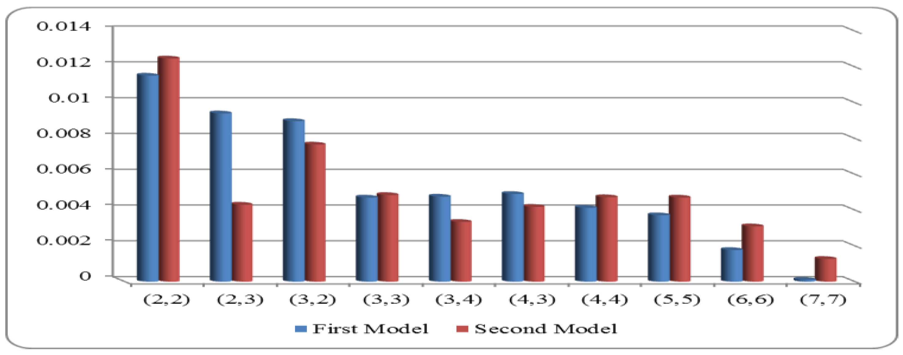
(n1, n2) (n1, n3)	True R	First Model			Second Model			RE
		${\widehat{\mathit{R}}}_1$	AB	MSE	${\widehat{\mathit{R}}}_2$	AB	MSE
(2, 2)	0.525	0.56868	0.04347	0.01729	0.50611	0.01910	0.00981	1.76
(2, 3)		0.49050	0.03470	0.00600	0.52290	0.00230	0.00380	1.58
(3, 2)		0.51268	0.01256	0.00876	0.64921	0.04112	0.00979	0.89
(3, 3)		0.51710	0.00814	0.00283	0.56285	0.03764	0.00605	0.47
(3, 4)		0.51665	0.00859	0.00654	0.55037	0.02516	0.00424	1.54
(4, 3)		0.50080	0.02440	0.00400	0.52175	0.00346	0.00375	1.07
(4, 4)		0.53195	0.00674	0.00459	0.58016	0.05495	0.00563	0.82
(5, 5)		0.51258	0.01266	0.00071	0.54453	0.01932	0.00361	0.20
(6, 6)		0.51445	0.01079	0.00064	0.57413	0.04891	0.00352	0.18
(7, 7)		0.50915	0.01610	0.00048	0.52627	0.00106	0.00118	0.41
(2, 2)	0.608	0.63588	0.02773	0.01371	0.59726	0.01083	0.01177	1.16
(2, 3)		0.55390	0.05420	0.00720	0.59570	0.01240	0.00310	2.32
(3, 2)		0.60754	0.00056	0.01069	0.64849	0.04041	0.00894	1.20
(3, 3)		0.52167	0.08643	0.00908	0.74632	0.03609	0.00510	1.78
(3, 4)		0.59465	0.01345	0.00468	0.64240	0.03431	0.00443	1.06
(4, 3)		0.57160	0.03650	0.00420	0.61624	0.008152	0.00280	1.50
(4, 4)		0.54436	0.06374	0.00427	0.62976	0.02167	0.00426	1.00
(5, 5)		0.61885	0.01070	0.00416	0.62782	0.01973	0.00261	1.59
(6, 6)		0.57038	0.03771	0.00370	0.63634	0.02825	0.00175	2.11
(7, 7)		0.60530	0.00285	0.00226	0.60895	0.00086	0.00130	1.74
(2, 2)	0.71	0.72385	0.01362	0.01151	0.63840	0.07183	0.01247	0.92
(2, 3)		0.65000	0.06030	0.00940	0.67300	0.03720	0.00430	2.19
(3, 2)		0.68619	0.02404	0.00897	0.74987	0.03965	0.00766	1.17
(3, 3)		0.76275	0.05252	0.00470	0.75806	0.04783	0.00484	0.97
(3, 4)		0.67922	0.03101	0.00475	0.74780	0.03758	0.00334	1.42
(4, 3)		0.67120	0.03910	0.00490	0.73876	0.02853	0.00418	1.17
(4, 4)		0.75943	0.04920	0.00413	0.72616	0.01593	0.00472	0.88
(5, 5)		0.71950	0.00927	0.00371	0.76365	0.05343	0.00470	0.79
(6, 6)		0.71257	0.00234	0.00177	0.74404	0.03381	0.00309	0.57
(7, 7)		0.70000	0.01023	0.00010	0.72248	0.01226	0.00127	0.08
(2, 2)	0.838	0.76102	0.07685	0.01825	0.81638	0.02149	0.00535	3.41
(2, 3)		0.79360	0.04430	0.00670	0.79100	0.04690	0.00460	1.46
(3, 2)		0.79422	0.04366	0.00858	0.87494	0.03706	0.00373	2.30
(3, 3)		0.77398	0.06389	0.00677	0.88606	0.04819	0.00393	1.72
(3, 4)		0.79285	0.04503	0.00609	0.89043	0.05255	0.00387	1.57
(4, 3)		0.80880	0.02900	0.00260	0.81064	0.02723	0.00324	0.80
(4, 4)		0.83720	0.00068	0.00261	0.88852	0.05065	0.00356	0.73
(5, 5)		0.84373	0.00574	0.00217	0.88288	0.04501	0.00318	0.68
(6, 6)		0.84532	0.00733	0.00124	0.86985	0.03198	0.00248	0.50
(7, 7)		0.85776	0.01989	0.00044	0.85442	0.01655	0.00093	0.47
(2, 2)	0.982	0.93803	0.04387	0.00480	0.96686	0.01514	0.00058	8.28
(2, 3)		0.95280	0.02920	0.00160	0.98458	0.00258	0.00004	40.00
(3, 2)		0.95787	0.02403	0.00120	0.99080	0.00879	0.00003	40.00
(3, 3)		0.96024	0.02166	0.00104	0.99070	0.00858	0.00003	34.67
(3, 4)		0.95881	0.02309	0.00109	0.98603	0.00403	0.00002	54.50
(4, 3)		0.95580	0.02610	0.00110	0.98721	0.00148	0.00001	110.00
(4, 4)		0.99142	0.00952	0.00015	0.98849	0.00649	0.00002	7.50
(5, 5)		0.98457	0.00257	0.00014	0.97239	0.00961	0.00001	14.00
(6, 6)		0.98235	0.00035	0.00011	0.98712	0.00512	0.00001	11.00
(7, 7)		0.99015	0.00825	0.00011	0.98537	0.00337	0.00001	11.00

.

From Table 7, we conclude that the MSE of ${\widehat{R}}_2$ is smaller than that of ${\widehat{R}}_1$ for true values of R = 0.982 and 0.608 in all of the cases. In conclusion, we find that the second model’s reliability estimator outperforms the first model, confirming the simulation observations.

8. Conclusions and Summary

This paper uses the MRSS approach to estimate stress–strength reliability for two models. The first model is investigated when the strength X and stress Y are distributed as Lomax with different shape parameters. In contrast, the second model is investigated when the strength X and stress Z are distributed according to Lomax and inverse Lomax, respectively, with different shape parameters and a similar scale parameter. For both models, the maximum likelihood estimators of $R$ are produced using MRSS. The R’s ML estimators are derived with similar or distinct set sizes in the two models. The performances of reliability estimators for both models are compared in light of numerical investigation. When both stress and strength have distinct set sizes, in most instances, the reliability estimates for the second model have smaller mean squared errors than those for the first model, according to the results of the numerical analysis. Furthermore, we found that for the same set size (even or odd), in some cases, the reliability estimate for the first model performs better than that obtained by the second model. As the set sizes become larger, the performance of all reliability estimates improves. In general, we may deduce that the first model is superior to the other model for dissimilar set sizes, whereas the first model is preferred over the second model for similar set sizes. The efficiency of all estimates improves as the set size increases. Medical data have been analyzed for more information, allowing the theoretical results to be confirmed. For future work, one can investigate the inference in a multicomponent S–S model [45,46] based on other modifications of RSS [47].

References

- Birnbaum, Z. On a use of the Mann-Whitney statistic. In Proceedings of the Third Berkeley Symposium on Mathematical Statistics and Probability, Berkley, CA, USA, 26–31 December 1956; pp. 13–17. [Google Scholar]
- Downton, F. The estimation of Pr(Y< X) in the normal case. Technometrics 1973, 15, 551–558. [Google Scholar]
- Constantine, K.; Tse, S.-K.; Karson, M. Estimation of P (Y<X) in the gamma case. Commun. Stat. Simul. Comput. 1986, 15, 365–388. [Google Scholar]
- Awad, A.M.; Gharraf, M.K. Estimation of P(Y<X) in the Burr case: A comparative study. Commun. Stat. Simul. Comput. 1986, 15, 389–403. [Google Scholar]
- Kundu, D.; Gupta, R.D. Estimation of P[Y<X] for generalized exponential distribution. Metrika 2005, 61, 291–308. [Google Scholar]
- Kundu, D.; Gupta, R.D. Estimation of P[Y<X] for Weibull distributions. IEEE Trans. Reliab. 2006, 55, 270–280. [Google Scholar]
- Hassan, A.S.; Al-Sulami, D. Estimation of P[Y<X] in the case of exponentiated Weibull distribution. Egypt Stat. J. 2008, 52, 76–95. [Google Scholar]
- Rao, G.S.; Aslam, M.; Kundu, D. Burr-XII distribution parametric estimation and estimation of reliability of multicomponent stress-strength. Commun. Stat. Theory Methods 2015, 44, 4953–4961. [Google Scholar] [CrossRef]
- Rao, G.S.; Bhatti, F.A.; Aslam, M.; Albassam, M. Estimation of reliability in a multicomponent stress–strength system for the exponentiated moment-based exponential distribution. Algorithms 2019, 12, 246. [Google Scholar] [CrossRef] [Green Version]
- Kotz, S.; Pensky, M. The Stress-Strength Model and Its Generalizations: Theory and Applications; World Scientific: Singapore, 2003. [Google Scholar]
- McIntyre, G.A. A method for unbiased selective sampling, using ranked sets. Aust. J. Agric. Res. 1952, 3, 385–390. [Google Scholar] [CrossRef]
- Takahasi, K.; Wakimoto, K. On unbiased estimates of the population mean based on the sample stratified by means of ordering. Ann. Inst. Stat. Math. 1968, 20, 1–31. [Google Scholar] [CrossRef]
- Zamanzade, E. EDF-based tests of exponentiality in pair ranked set sampling. Stat. Pap. 2019, 60, 2141–2159. [Google Scholar] [CrossRef]
- Alghamdi, S.M.; Bantan, R.A.; Hassan, A.S.; Nagy, H.F.; Elbatal, I.; Elgarhy, M. Improved EDF-based tests for Weibull distribution using ranked set sampling. Mathematics 2022, 10, 4700. [Google Scholar] [CrossRef]
- Muttlak, H.A. Median ranked set sampling. J. Appl. Stat. Sci. 1997, 6, 245–255. [Google Scholar]
- Hajighorbani, S.; Aliakbari Saba, R. Stratified median ranked set sampling: Optimum and proportional allocations. J. Stat. Res. Iran JSRI 2012, 9, 87–102. [Google Scholar] [CrossRef] [Green Version]
- Sengupta, S.; Mukhuti, S. Unbiased estimation of P(X>Y) for exponential populations using order statistics with application in ranked set sampling. Commun. Stat. Theory Methods 2008, 37, 898–916. [Google Scholar] [CrossRef]
- Muttlak, H.A.; Abu-Dayyeh, W.A.; Saleh, M.F.; Al-Sawi, E. Estimating P(Y<X) using ranked set sampling in case of the exponential distribution. Commun. Stat. Theory Methods 2010, 39, 1855–1868. [Google Scholar]
- Akgül, F.G.; Şenoğlu, B. Estimation of P (X<Y) using ranked set sampling for the Weibull distribution. Qual. Technol. Quant. Manag. 2017, 14, 296–309. [Google Scholar]
- Akgül, F.G.; Acıtaş, Ş.; Şenoğlu, B. Inferences on stress–strength reliability based on ranked set sampling data in case of Lindley distribution. J. Stat. Comput. Simul. 2018, 88, 3018–3032. [Google Scholar] [CrossRef]
- Safariyan, A.; Arashi, M.; Arabi Belaghi, R. Improved point and interval estimation of the stress–strength reliability based on ranked set sampling. Statistics 2019, 53, 101–125. [Google Scholar] [CrossRef]
- Al-Omari, A.I.; Almanjahie, I.M.; Hassan, A.S.; Nagy, H.F. Estimation of the stress-strength reliability for exponentiated Pareto distribution using median and ranked set sampling methods. Comput. Mater. Contin. 2020, 64, 835–857. [Google Scholar]
- Esemen, M.; Gurler, S.; Sevinc, B. Estimation of stress–strength reliability based on ranked set sampling for generalized exponential distribution. Int. J. Reliab. Qual. Saf. Eng. 2021, 28, 2150011. [Google Scholar] [CrossRef]
- Hassan, A.S.; Al-Omari, A.I.; Nagy, H.F. Stress–Strength reliability for the generalized inverted exponential distribution using MRSS. Iran. J. Sci. Technol. Trans. A Sci. 2021, 45, 641–659. [Google Scholar] [CrossRef]
- Al-Omari, A.I.; Hassan, A.S.; Alotaibi, N.; Shrahili, M.; Nagy, H.F. Reliability estimation of inverse Lomax distribution using extreme ranked set sampling. Adv. Math. Phys. 2021, 2021, 4599872. [Google Scholar] [CrossRef]
- Yousef, M.M.; Hassan, A.S.; Al-Nefaie, A.H.; Almetwally, E.M.; Almongy, H.M. Bayesian estimation using MCMC method of system reliability for inverted Topp-Leone distribution based on ranked set sampling. Mathematics 2022, 10, 3122. [Google Scholar] [CrossRef]
- Hassan, A.S.; Elshaarawy, R.S.; Onyango, R.; Nagy, H.F. Estimating system reliability using neoteric and median RSS data for generalized exponential distribution. Int. J. Math. Math. Sci. 2022, 2022, 2608656. [Google Scholar] [CrossRef]
- Wu, W.; Wang, B.X.; Chen, J.; Miao, J.; Guan, Q. Interval estimation of the two-parameter exponential constant stress accelerated life test model under Type-II censoring. Qual. Technol. Quant. Manag. 2022. [Google Scholar] [CrossRef]
- Abbas, K.; Tang, Y. Objective Bayesian analysis of the Frechet stress–strength model. Stat. Probab. Lett. 2014, 84, 169–175. [Google Scholar] [CrossRef]
- Zhang, L.; Xu, A.; An, L.; Li, M. Bayesian inference of system reliability for multicomponent stress-strength model under Marshall-Olkin Weibull distribution. Systems 2022, 10, 196. [Google Scholar] [CrossRef]
- Zhuang, L.; Xu, A.; Wang, B.; Xue, Y.; Zhang, S. Data analysis of progressive-stress accelerated life tests with group effects. Qual. Technol. Quant. Manag. 2022. [Google Scholar] [CrossRef]
- Bryson, M.C. Heavy-tailed distributions: Properties and tests. Technometrics 1974, 16, 61–68. [Google Scholar] [CrossRef]
- Balkema, A.A.; De Haan, L. Residual life time at great age. Ann. Probab. 1974, 2, 792–804. [Google Scholar] [CrossRef]
- Chahkandi, M.; Ganjali, M. On some lifetime distributions with decreasing failure rate. Comput. Stat. Data Anal. 2009, 53, 4433–4440. [Google Scholar] [CrossRef]
- Hassan, A.S.; Al-Ghamdi, A.S. Optimum step stress accelerated life testing for Lomax distribution. J. Appl. Sci. Res. 2009, 51, 2153–2164. [Google Scholar]
- Johnson, N.L.; Kotz, S.; Balakrishnan, N. Continuous Univariate Distributions; John Wiley & Sons, Inc.: New York, NY, USA, 1994; Volume 1. [Google Scholar]
- Ahsanullah, M. Record values of the Lomax distribution. Stat. Neerl. 1991, 45, 21–29. [Google Scholar] [CrossRef]
- Hassan, A.S.; Zaky, A.N. Entropy Bayesian estimation for Lomax distribution based on record. Thail. Stat. 2021, 19, 95–114. [Google Scholar]
- Helmy, B.A.; Hassan, A.S.; El-Kholy, A.K. Analysis of uncertainty measure using unified hybrid censored data with applications. J. Taibah Univ. Sci. 2021, 15, 1130–1143. [Google Scholar] [CrossRef]
- Kleiber, C.; Kotz, S. Statistical Size Distributions in Economics and Actuarial Sciences; John Wiley & Sons, Inc.: Hoboken, NJ, USA, 2003; Volume 470. [Google Scholar]
- Ge, S.; McKenzie, J.; Voss, C.; Wu, Q. Exchange of groundwater and surface-water mediated by permafrost response to seasonal and long term air temperature variation. Geophys. Res. Lett. 2011, 38, 1–6. [Google Scholar] [CrossRef] [Green Version]
- Singh, S.K.; Singh, U.; Yadav, A.S. Reliability estimation for inverse Lomax distribution under type Π censored data using Markov chain Monte Carlo method. Int. J. Math. Stat. 2016, 17, 128–146. [Google Scholar]
- Yadav, A.S.; Singh, S.K.; Singh, U. On hybrid censored inverse Lomax distribution: Application to the survival data. Statistica 2016, 76, 185–203. [Google Scholar]
- Efron, B. Logistic regression, survival analysis, and the Kaplan-Meier curve. J. Am. Stat. Assoc. 1988, 83, 414–425. [Google Scholar] [CrossRef]
- Hassan, A.S.; Nagy, H.F. Reliability estimation in multicomponent stress-strength for generalized inverted exponential distribution based on ranked set sampling. Gazi Univ. J. Sci. 2022, 35, 314–331. [Google Scholar]
- Hassan, A.S.; Nagy, H.F.; Muhammed, H.Z.; Saad, M.S. Estimation of multicomponent stress-strength reliability following Weibull distribution based on upper record values. J. Taibah Univ. Sci. 2020, 14, 244–253. [Google Scholar] [CrossRef] [Green Version]
- Hassan, A.S.; Elshaarawy, R.S.; Nagy, H.F. Parameter estimation of exponentiated exponential distribution under selective ranked set sampling. Stat. Transit. New Ser. 2022, 23, 37–58. [Google Scholar] [CrossRef]