Deep Learning Method Based on Physics-Informed Neural Network for 3D Anisotropic Steady-State Heat Conduction Problems

Abstract

This paper uses the physical information neural network (PINN) model to solve a 3D anisotropic steady-state heat conduction problem based on deep learning techniques. The model embeds the problem’s governing equations and boundary conditions into the neural network and treats the neural network’s output as the numerical solution of the partial differential equation. Then, the network is trained using the Adam optimizer on the training set. The output progressively converges toward the accurate solution of the equation. In the first numerical example, we demonstrate the convergence of the PINN by discussing the effect of the neural network’s number of layers, each hidden layer’s number of neurons, the initial learning rate and decay rate, the size of the training set, the mini-batch size, the amount of training points on the boundary, and the training steps on the relative error of the numerical solution, respectively. The numerical solutions are presented for three different examples. Thus, the effectiveness of the method is verified.

1. Introduction

Deep learning methods are an efficient means of solving partial differential equations (PDEs), which describe many natural phenomena and processes in modern engineering, such as fluid mechanics, electromagnetism, quantum mechanics, etc. [1,2]. The governing equation of anisotropic heat conduction problems differs from isotropic problems because the mixed partial derivatives exist [3]. The deep learning method program is simple to implement and does not require the generation of meshes [4,5]. Therefore, it is of great significance and value to study deep learning methods for heat transfer problems [6,7].

With the increasing application of various anisotropic materials in engineering practice, the requirements for the numerical simulation and calculation of heat conduction are also increasing, and these problems are usually modeled by using partial differential equations and solved using numerical methods. The finite element method (FEM) [8,9] and the boundary element method (BEM) [10,11] are important numerical methods and have been applied to a lot of complicated problems [12,13]. The methods are based on mesh generation, require highly discrete meshes to model the problem, transform the original problem into a system of algebraic equations, and then obtain numerical solutions by solving algebraic equations [14,15]. These methods have been developed for decades and are quite mature in dealing with complex problems. However, the numerical solution’s computational efficiency and accuracy depend on the meshing’s quality. For complex geometries in three-dimensional space, the fineness of the mesh must be increased to achieve higher numerical accuracy. As the number of meshes increases, it raises labor costs to divide the mesh, and the computational cost will increase significantly.

Meshless methods are point-based approximations that avoid the drawbacks due to the mesh [16,17,18], and they have been applied to solve many problems in science and engineering fields [19,20,21,22]. Several meshless methods have been developed for solving heat conduction problems in recent years. Cheng et al. [23,24,25] presented meshless methods for solving the inverse heat conduction problem with a source parameter. Chen et al. [26,27,28] proposed the complex variable reproducing kernel particle method and the complex variable element-free Galerkin (CVEFG) method for transient heat conduction problems. Researchers have developed meshless methods to obtain numerical solutions to anisotropic heat transfer problems. Gu et al. [29] have solved 3D anisotropic heat conduction problems by the singular boundary method (SBM). Lu et al. [30] proposed the modified scaled boundary finite element method and then extended it to address layered heat conduction problems with an anisotropic medium. Guan et al. [31] analyzed non-homogeneous anisotropic heat conduction problems by the fragility point methods based on Petrov–Galerkin weak forms. The authors established the local approximation using the differential quadrature method based on the radial basis function. Shiah et al. [32] proposed a boundary integral equation using a domain mapping technique and multiple reciprocity method to solve three-dimensional anisotropic heat conduction problems. Gu et al. [33] proposed the meshless localized fundamental solutions method for 3D anisotropic heat conduction modeling on a large scale. Zhang et al. [34] studied a transient heat conduction simulation of anisotropic materials based on the EFG method, which has higher numerical solution accuracy. However, the EFG method will inevitably result in singular matrices during the calculation process, leading to a slower calculation. Thus, the improved element-free Galerkin (IEFG) method is proposed using the orthogonal basis function. Zhang et al. [35] studied the partial differential equations for 3D transient heat conduction using the IEFG method. Cheng et al. [36] studied the IEFG method to solve two-dimensional anisotropic heat conduction problems. The numerical solutions show that the IEFG method has a quicker computational speed. The EFG, IEFG, and CVEFG methods are based on the moving least-squares (MLS) approximation. The MLS approximation is obtained from the least-squares method in mathematics [37,38,39]. And the least-squares method has been applied to many problems [40,41] because it can results in the best approximation.

In EFG, IEFG, and CVEFG methods, essential boundary conditions are typically imposed via the penalty or Lagrange multiplier methods. To directly impose essential boundary conditions, researchers have proposed the interpolated EFG method [42,43,44] for increasing the computational speed and accuracy of the IEFG method.

To enhance the efficiency of the IEFG method to solve 3D heat conduction problems, a dimensional splitting meshless method [45,46,47,48] is proposed, where the three-dimensional problem is split into a series of two-dimensional problems. These 2D problems are solved by employing the meshless method, which the FDM treats in a splitting direction, and the numerical solution shows that the dimensional splitting meshless method effectively enhances the computational speed of the IEFG method for three-dimensional problems. Although the dimensional splitting meshless methods can mitigate the drawbacks of mesh-based partitioning and have a higher calculation speed, they still require complex formula derivation and pose additional programming complexity when solving three-dimensional problems.

With the development of computer technology, a machine learning technique called physical information neural network (PINN) has been used to solve mathematical equations and physics problems [49,50]. The PINN introduces neural networks into numerical simulations and transforms the solution of PDEs into unsupervised learning problems. Many scholars have used it to solve 3D heat conduction problems by integrating the governing equations of the physical problem with its boundary conditions or initial conditions into a neural network. Then, the solution of PDEs is approximated by training the neural network to minimize the loss function.

In the present study, we use the PINN to solve the anisotropic steady-state heat conduction problem in three dimensions by embedding boundary conditions and governing equations of the heat transfer problem into a neural network, treating the neural network’s output as a numerical solution of a partial differential equation. We use the Adam method to optimize network parameters, and the network is trained to minimize the loss function. Thus, the output of the network gradually approximates the exact solution.

The effects of the neural network structure, initial learning rate, decay rate, training epochs, number of sampling points on the boundary, size of the training set, and mini-batch size on numerical accuracy in small-batch training are discussed through numerical examples, and the convergence of the PINN is demonstrated numerically. The results from numerical examples verify the effectiveness of the PINN in solving the anisotropic steady-state heat conduction problem in three dimensions.

2. Equations of 3D Anisotropic Steady-State Heat Conduction Problems

The equation governing the steady-state heat conduction problem in a three-dimensional anisotropic system can be written as

$$\nabla (k\nabla u(x))=Q, (\mathit{x}=(x_1,x_2,x_3)\in \mathsf{\Omega }),$$

(1)

The boundary conditions are

$$u(\mathit{x})=\overline{u}(\mathit{x}), (\mathit{x}\in {\mathsf{\Gamma }}_u),$$

(2)

$$\mathit{q}(\mathit{x})=-\mathit{k}\nabla u(\mathit{x})\cdot \mathit{n}=\overline{\mathit{q}}(\mathit{x}), (\mathit{x}\in {\mathsf{\Gamma }}_q),$$

(3)

where $u(x)$ is a function representing the temperature distribution of the thermal field, $Q$ represents the rate at which internal heat source is generated, $\overline{u}$ and $\overline{q}$ are given function values, $\mathsf{\Gamma }={\mathsf{\Gamma }}_u\cup {\mathsf{\Gamma }}_q$, ${\mathsf{\Gamma }}_u\cap {\mathsf{\Gamma }}_q=\varnothing$, and n is the outward normal to the boundary at x. And k is a symmetric matrix, k: = k_ij (k_ij = k_ji), 1 ≤ i, j ≤ n, n is the space dimension, and k_ij is the thermal conductivity. In the three-dimensional problem n = 3, thus k₁₁, k₂₂, and k₃₃ represent thermal conductivities in three directions, and k₁₂, k₁₃, k₂₃ represent thermal conductivities in the Ox_{1 × 2}, Ox₁x₃, and Ox₂x₃ planes, respectively. According to the principles of thermodynamics and Onsager reciprocal relations, the thermal conductivity coefficients satisfy the following equation

$$k_{ii}>0, (i=1,2,3); k_{11}{k}_{22}>k_{12}^2; k_{22}{k}_{33}>k_{23}^2; k_{33}{k}_{11}>k_{31}^2.$$

(4)

In 3D anisotropic heat conduction problems, the governing equations and their coefficients represent the physical process of heat conduction by distinguishing the strengths of heat conduction in different directions. This distinction is beneficial to understanding the conduction mechanism in anisotropic materials thoroughly. In practical engineering applications, the heat conduction equation is an important mathematical model for various thermal problems and heat transfer design issues. Determining boundary conditions is crucial for solving heat conduction problems as it allows for a better simulation of real-world engineering scenarios.

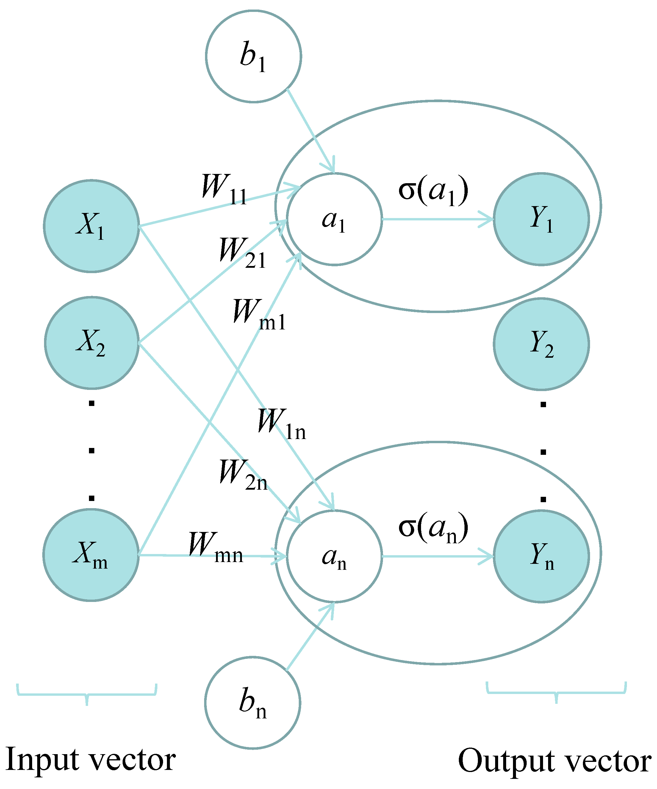
3. The PINN for 3D Anisotropic Steady-State Heat Conduction Problem

Typically, within the framework of the PINN, a feed-forward, fully connected neural network approximation is employed [49], indicated as $\xi (\mathit{x};\mathit{\theta })$, which is considered to approximate $u(x)$, where x (x₁, x₂, x₃) is the independent variable of the partial differential equation as input, and θ denotes the weight and bias of the numerical transmission between neurons. The output U of the neural network is considered the PDE’s solution.

$$U=\xi (\mathit{x};\mathit{\theta }).$$

(5)

The structure of a feed-forward, fully connected neural network is shown in Figure 1. The architecture consists of an input layer with three neurons, several hidden layers, and an output layer with a single neuron. Each neuron in both the upper and lower layers is connected, and the purpose of these connections is to transfer information between neurons. It can map input coordinates (points in 3D space) to outputs (solutions to partial differential equations).

The detailed configuration of hidden layers is illustrated in Figure 2. For each layer, the input vector has a relationship with the output vector as

$$Y_i=\sigma ({\displaystyle \sum _{j=1}^m{W}_{ji}{X}_j}+b_i), (i=1,2,\cdots n).$$

(6)

The previous layer has m neurons, and the next layer has n neurons, where W_ji and b_i represent the parameters for transmitting neuronal information, W_ji is weight, and b_i is bias, which represents the weight of the contribution of the j-th neuron in the previous layer to the i-th neuron in the next layer. Adjusting the activation threshold of the weighted sum of neurons in the previous layer for the i-th neuron in the next layer, respectively, they are also trainable parameters. X_j denotes the value of the j-th neuron in the previous layer, and Y_i denotes the value of the i-th neuron in the next layer.

The σ represents the activation function of a simple nonlinear transformation, while some activation functions are relu, sigmoid, tanh, etc., where the tanh activation function is symmetric, with its function image shown in Figure 3, and its functional form is Equation (7). It can be used for second-order or higher-order partial differential equations. Therefore, the tanh function is used in this study [49].

$$\sigma (a)=\frac{e^a-e^{-a}}{e^a+e^{-a}}.$$

(7)

In order to train the neural network, some training data need to be prepared. The dataset consists of N_f discrete points inside the solution domain (xⁱ= x₁ⁱ, x₂ⁱ, x₃ⁱ, i = 1,2,…,N_f) and N_b discrete points on the boundary (x^j= x₁^j, x₂^j, x₃^j, j = 1,2,…,N_b). The discrete points in the interior are generated based on the Sobol sequence and the discrete points on the boundary are uniformly sampled.

The quasi-random numbers of the Sobol sequence are more uniform than traditional pseudo-random number generators in higher dimensional cases [51]. Figure 4 shows the distribution of internal discrete points in space. It can be seen that these points are uniformly distributed in three dimensions.

During the training of a neural network, the gap between the output of the model and the true value is measured by defining an appropriate loss function. We define an f function as follows:

$$f=k_{11}\frac{{\partial }^{2}U}{\partial x_1^2}+k_{22}\frac{{\partial }^{2}U}{\partial x_2^2}+k_{33}\frac{{\partial }^{2}U}{\partial x_3^2}+2k_{12}\frac{{\partial }^{2}U}{\partial x_1\partial x_2}+2k_{23}\frac{{\partial }^{2}U}{\partial x_2\partial x_3}+2k_{31}\frac{{\partial }^{2}U}{\partial x_3\partial x_1}-Q.$$

(8)

The zeros of the f function are the solutions of the governing equation, so the loss term of the governing equation is given as

$$los{s}_f=\frac{1}{N_f}{\displaystyle \sum _{i=1}^{N_f}{\left|f(x^i)-0\right|}^2}.$$

(9)

The loss_f is the mean square error of the f function value with respect to zero, and it can characterize the gap between the left and right terms of the governing equation (Equation (1)), where N_f represents the number of discrete points taken inside the solution domain.

$$los{s}_b=\frac{1}{N_{\mathrm{b}}}{\displaystyle \sum _{j=1}^{N_{\mathrm{b}}}{\left|U(x^j)-\overline{u}\left(x^j\right)\right|}^2}.$$

(10)

The loss_b is the mean square error between the predicted value and the true value at the boundary point, and it can characterize the gap between the model’s output at the boundary and the actual value, where N_b represents the number of discrete points taken on the boundary.

Thus, the total loss function is the sum of the following two terms:

$$loss=los{s}_f+los{s}_{\mathrm{b}}.$$

(11)

Next, the network can be trained. Automatic differentiation is used to obtain the first-order and second-order derivatives of the numerical solution to the independent variables, and then we can calculate the loss. The gradient of the loss to θ (${\nabla }_{\theta }loss$) is back-propagated.

$${\nabla }_{\theta }loss={\left({\left(\frac{\partial loss}{\partial {\theta }_1}\right)}^{\mathrm{T}},{\left(\frac{\partial loss}{\partial {\theta }_2}\right)}^{\mathrm{T}},\cdots ,{\left(\frac{\partial loss}{\partial {\theta }_{L-1}}\right)}^{\mathrm{T}}\right)}^{\mathrm{T}}, {\mathit{\theta }}_I={({({\mathit{W}}^{(I)})}^{\mathrm{T}},{({\mathit{b}}^{(I)})}^{\mathrm{T}})}^{\mathrm{T}},$$

$$I=1,2,\cdots ,L-1,$$

(12)

where W^(I) and b^(I) represent the weights and bias column vectors of I-th layer, respectively.

The Adam optimization updates the network parameters to minimize the loss function [52]. Once the loss function has converged, the network can obtain a numerical solution that satisfies the requirements. Using the Adam optimizer, we can speed up the model’s training and avoid gradient disappearance or explosion. The rule for updating the parameters is as follows:

$${\theta }_{t+1}={\theta }_t-\alpha \frac{m_t}{\sqrt{v_t}+\epsilon },$$

(13)

where θ_t is the network parameter at step t, α is the learning rate, m_t and v_t are the first-order and second-order momentum estimates, respectively, and ε is a very small positive number to prevent division-by-zero errors; it takes the value 1 × 10⁻⁸.

After updating the parameters, we will perform forward and backward propagation again, and this process will be iterated until a predetermined number of training sessions is reached or the training reaches a certain level of accuracy. We can obtain a model that can fit the data by continuously optimizing the parameter updates. Eventually, the relative error between the output of the computed test data and the exact solution is calculated. If the error approaches zero, it can be considered that the network has learned the solution to the equation.

Thus, the PINN’s structure for solving 3D anisotropic heat conduction problems can be represented (see Figure 5).

The specific procedure for the PINN to solve the 3D anisotropic steady-state heat conduction is as follows, Algorithm 1:

Algorithm 1 Algorithmic Procedure
Input: Internal training data, (xi); boundary training data, (xj);
Output: Prediction of DNN, $\xi (\mathit{x};\mathit{\theta })$;
1:	Initialize the parameters of DNN;
2:	Define the loss function: loss = lossf + lossb;
3:	for epoch = 1:numEpochs
4:	U1 = ξ (xi; θ), ξ (xj; θ);
5:	compute loss;
6:	obtain gradients by automatic differential;
7:	minimize the loss by Adam method;
8:	end;
9:	Obtain the prediction U = ξ (xk; θ);
10:	return U.

4. Numerical Examples

This section presents three numerical experiments related to anisotropic heat conduction problems in three dimensions. We will calculate the relative error of the PINN to verify the effectiveness of the PINN for the problems, and so the relative error equation is defined as

$$\mathrm{Error}=\frac{{\left({\displaystyle \sum _{k=1}^{N_k}{\left|\mathit{U}({\mathit{x}}^k)-\mathit{u}({\mathit{x}}^k)\right|}^2}\right)}^{\frac{1}{2}}}{{\left({\displaystyle \sum _{k=1}^{N_k}{\left|\mathit{u}({\mathit{x}}^k)\right|}^2}\right)}^{\frac{1}{2}}},$$

(14)

where x^k(x₁^k, x₂^k, x₃^k) are discrete points in the test set, N_k denotes the number of points in the test set, U(x^k) denotes the predicted value of the test point, and u(x^k) denotes the actual value of the test point.

The PINN solves three numerical cases by encoding the governing equations and boundary conditions into a neural network, treating the neural network’s output as a numerical solution of the partial differential equation. Then, the neural network is trained so that the solution of the equation is approached progressively by the output.

The first example is

$$\frac{{\partial }^{2}u}{\partial x_1^2}+\frac{{\partial }^{2}u}{\partial x_2^2}+\frac{{\partial }^{2}u}{\partial x_3^2}+\frac{{\partial }^{2}u}{\partial x_1\partial x_2}+\frac{{\partial }^{2}u}{\partial x_2\partial x_3}+\frac{{\partial }^{2}u}{\partial x_3\partial x_1}=0.$$

(15)

This problem domain is $\mathsf{\Omega }={[0,1]}^3$.

The boundary conditions are

$${u|}_{x_1=0}=0.5x_2^2-1.5x_3^2+0.5x_2{x}_3+2,$$

(16)

$${u|}_{x_2=0}=0.5x_1^2-1.5x_3^2+x_1{x}_3+2,$$

(17)

$${u|}_{x_3=0}=0.5x_1^2+0.5x_2^2-0.5x_1{x}_2+2,$$

(18)

$${u|}_{x_1=1}=0.5+0.5x_2^2-1.5x_3^2-0.5x_2+x_3+0.5x_2{x}_3+2,$$

(19)

$${u|}_{x_2=1}=0.5x_1^2+0.5-1.5x_3^2-0.5x_1+x_1{x}_3+0.5x_3+2,$$

(20)

$${u|}_{x_3=1}=0.5x_1^2+0.5x_2^2-1.5-0.5x_1{x}_2+x_1+0.5x_2+2.$$

(21)

The theoretical result is

$$u=0.5x_1^2+0.5x_2^2-1.5x_3^2-0.5x_1{x}_2+x_1{x}_3+0.5x_2{x}_3+2.$$

(22)

This study will investigate the effect of various factors on the relative error of the numerical solution obtained by a neural network. These factors include the neural network’s number of layers, which impacts its capacity to capture complex relationships in the data [53]. The number of neurons in each hidden layer influences the network’s representational power and ability to learn high-level features. The initial learning rate and the decay value determine the rate at which the network adjusts its weights during training. The size of the training set and the mini-batch size affect the generalization capability and training efficiency of the network. Additionally, the amount of training points on the boundary and the number of training steps impact the network’s ability to approximate the boundary accurately. By examining these factors, we can gain insights into their influence on the accuracy and performance of the numerical solution.

The most critical factor influencing the relative error is the structure of a neural network. We have shown the relative error of the numerical solution using different combinations of the neural network’s number of layers and each hidden layer’s number of neurons, from three to eight layers and four to twelve neurons. As shown in Figure 6, the smaller relative error of a numerical solution can be achieved with a neural network with five layers and nine neurons.

Furthermore, the initial learning and decay rates directly impact the network’s training performance; thus, we have investigated the effect of different initial and decay learning rates on the relative error. The error is minimized for the initial value of the learning rate as 0.03 and the decay rate as 0.005 (Figure 7).

In this study, the boundary conditions of problems are embedded within the neural network. Consequently, we investigate the effect of the number of training points on each boundary of the problem domain on the relative error of the numerical solution (Figure 8). The results indicate that a small relative error can be obtained when the number of training points on each boundary surface of the problem domain is set to 19 × 19.

This study uses a small-batch training method to divide the training data into multiple small batches for model parameter updates. Only the current small batch of data is used for parameter tuning with each update to improve training efficiency and potentially improve model performance and generalization. We have investigated the impact of training sets of different sizes and batch configurations on the relative error (Figure 9). The results show that a small relative error can be achieved when the training set comprises 100 discrete points divided into four batches.

Figure 10 shows how the numerical solution’s relative error varies as the iteration steps increase during the network training. The results indicate that the relative error will no longer decrease after the iteration steps exceed 2500.

Therefore, the neural network is structured with three hidden layers and nine neurons per layer. An initial learning rate of 0.03 and a decay value of 0.005 are specified. The training set comprises 100 discrete points generated by the Sobol sequence, divided into four small batches to improve training efficiency. We sampled 19 × 19 points on each cube-shaped problem domain boundary surface. The test set comprises 11 × 11 × 11 discrete points uniformly distributed in the problem domain. The results showed that the numerical solution’s relative error is 0.0722% with 2500 training steps.

Figure 11, Figure 12 and Figure 13 compare the numerical and analytical solutions on a certain line in three different directions, respectively. Figure 14 and Figure 15 show the numerical and analytical solutions’ distribution on the plane where x₃ = 0.25, respectively.

There is a good agreement between the numerical solutions yielded by the PINN and the analytical solutions.

It can be seen that the numerical solutions obtained by the PINN are very close to the analytical solutions.

The second example is

$$\frac{{\partial }^{2}u}{\partial x_1^2}+0.8\frac{{\partial }^{2}u}{\partial x_2^2}+0.6\frac{{\partial }^{2}u}{\partial x_3^2}+0.2\frac{{\partial }^{2}u}{\partial x_1\partial x_2}+0.6\frac{{\partial }^{2}u}{\partial x_2\partial x_3}+0.4\frac{{\partial }^{2}u}{\partial x_3\partial x_1}=0.$$

(23)

This problem domain is $\mathsf{\Omega }={[0,1]}^3$.

The boundary conditions are

$${u|}_{x_1=0}=0.25x_2^2+\frac{5}{12}{x}_3^2-x_2{x}_3,$$

(24)

$${u|}_{x_1=1}=0.15+0.25x_2^2+\frac{5}{12}{x}_3^2-x_2-x_3-x_2{x}_3,$$

(25)

$${u|}_{x_2=0}=0.15x_1^2+\frac{5}{12}{x}_3^2-x_1{x}_3,$$

(26)

$${u|}_{x_2=1}=0.15x_1^2+0.25+\frac{5}{12}{x}_3^2-x_1-x_1{x}_3-x_3,$$

(27)

$${u|}_{x_3=0}=0.15x_1^2+0.25x_2^2-x_1{x}_2,$$

(28)

$${u|}_{x_3=1}=0.15x_1^2+0.25x_2^2+\frac{5}{12}-x_1{x}_2-x_1-x_2.$$

(29)

The theoretical result is

$$u=0.15x_1^2+0.25x_2^2+(5/12)x_3^2-x_1{x}_2-x_1{x}_3-x_2{x}_3.$$

(30)

For this example, we set the structure of the neural network as three hidden layers with eight neurons in each layer. The initial learning rate value is 0.01, and the decay value is 0.005. The training set uses 100 discrete points generated from the Sobol sequence, and then a small-batch training method is used to improve the training efficiency, and each batch is set to 20 discrete points. The 11 × 11 training points are taken on each boundary surface of the cube-shaped problem domain, and then we adopt the Adam optimizer for training the PINN.

The PINN was trained using 20,000 epochs of the training data, and the test set comprises 11 × 11 × 11 discrete points uniformly distributed in the problem domain to obtain a small relative error of the numerical solution of 0.4925%.

The numerical solutions of the PINN were contrasted with the analytical ones shown in Figure 16, Figure 17 and Figure 18 which show the numerical and analytical solutions compared on a certain line in three perpendicular directions, respectively. The numerical and analytical solutions distributed on the plane of x₃ = 0.25 are shown in Figure 19 and Figure 20, respectively.

It is visually apparent that the numerical solutions obtained through the PINN closely correspond to the analytical solutions.

The third example is

$${10}^{-4}\frac{{\partial }^{2}u}{\partial x_1^2}+{10}^{-4}\frac{{\partial }^{2}u}{\partial x_2^2}+{10}^{-4}\frac{{\partial }^{2}u}{\partial x_3^2}+2\times {10}^{-5}\frac{{\partial }^{2}u}{\partial x_2\partial x_3}=0.$$

(31)

This problem domain is $\mathsf{\Omega }={[0,1]}^3$.

The boundary conditions are

$${u|}_{x_1=0}=x_2^2+x_2-5x_2{x}_3,$$

(32)

$${u|}_{x_1=1}=x_2^2+x_2+x_3-5x_2{x}_3,$$

(33)

$${u|}_{x_2=0}=x_1{x}_3,$$

(34)

$${u|}_{x_2=1}=2+x_1{x}_3-5x_3,$$

(35)

$${u|}_{x_3=0}=x_2^2+x_2,$$

(36)

$${u|}_{x_3=1}=x_2^2+x_2+x_1-5x_2.$$

(37)

The theoretical result is

$$u=x_2^2+x_2+x_1{x}_3-5x_2{x}_3$$

(38)

For this example, the neural network is constructed by two hidden layers and nine neurons in every layer; the initial value of the learning rate is 0.03 and the decay value is 0.005. The training set uses 100 discrete points generated from the Sobol sequence. The training process uses a small-batch method to improve efficiency, with each batch containing 20 discrete points. Sampling is taken on each cube-shaped problem domain boundary surface at 11 × 11 points. Finally, the PINN training is optimized with the Adam optimizer.

The PINN was trained using 5000 epochs of the training data. The test set comprises 11 × 11 × 11 discrete points uniformly distributed in the problem domain. As a result, a small relative error of 0.2279% can be obtained for the numerical solution.

The numerical solutions of the PINN are compared with the analytical ones and are shown in Figure 21, Figure 22 and Figure 23 which show the comparison between the numerical and analytic solutions on a certain line in three different directions. Figure 24 and Figure 25 show the distribution of numerical and analytic solutions on a plane of x₃ = 0.25, respectively.

A visual inspection confirms that the numerical solutions obtained by using the PINN provide a high level of agreement with the analytical solutions, indicating the efficacy of the PINN in solving 3D anisotropic heat conduction problems with great computational accuracy.

5. Conclusions

This study utilizes the PINN to solve anisotropic steady-state heat conduction problems in three dimensions. By integrating the neural network into the numerical simulation process, the PINN incorporates the problem’s governing equations and boundary conditions into the network, treating the neural network’s output as the numerical solution of the PDE. Additionally, the PINN transforms the solution of a partial differential equation into an unsupervised learning problem and trains the network to minimize the loss function. The effectiveness of the PINN in solving the 3D anisotropic heat conduction problem is demonstrated through numerical examples.

Physical information neural networks offer a simple and efficient approach to solving challenging problems without the need for complex formula derivations. These networks utilize clear and simple codes and can conduct efficient parallel computations. The high flexibility allows physical information neural networks to tackle various scenarios and numerical computation problems easily.

While neural networks perform well in function fitting, their limitations require further research and development. Therefore, future efforts must be focused on exploring novel algorithms and techniques to improve the generalization ability, decrease training time, and increase the interpretability of neural networks.

References

1. Arora, G.; Joshi, V. A computational approach for solution of one dimensional parabolic partial differential equation with application in biological processes. Ain Shams Eng. J. 2018, 9, 1141–1150. [Google Scholar] [CrossRef]
2. Koroche, K.A. Numerical solution for one dimensional linear types of parabolic partial differential equation and application to heat equation. Math. Comput. Sci. 2020, 5, 76. [Google Scholar] [CrossRef]
3. Voinea-Marinescu, A.P.; Marin, L. Fading regularization MFS algorithm for the Cauchy problem in anisotropic heat conduction. Comput. Mech. 2021, 68, 921–941. [Google Scholar] [CrossRef]
4. Li, Y.; Zhou, Z.; Ying, S. DeLISA: Deep learning based iteration scheme approximation for solving PDEs. J. Comput. Phys. 2022, 451, 110884. [Google Scholar] [CrossRef]
5. Li, Y.; Xu, L.; Ying, S. DWNN: Deep wavelet neural network for solving partial differential equations. Mathematics 2022, 10, 1976. [Google Scholar] [CrossRef]
6. Zhu, J.-A.; Jia, Y.; Lei, J.; Liu, Z. Deep learning approach to mechanical property prediction of single-network hydrogel. Mathematics 2021, 9, 2804. [Google Scholar] [CrossRef]
7. Zheng, S.; Liu, Z. The machine learning embedded method of parameters determination in the constitutive models and potential applications for hydrogels. Int. J. Appl. Mech. 2021, 13, 2150001. [Google Scholar] [CrossRef]
8. Huang, R.; Zheng, S.; Liu, Z.; Ng, T.Y. Recent advances of the constitutive models of smart materials—Hydrogels and shape memory polymers. Int. J. Appl. Mech. 2020, 12, 2050014. [Google Scholar] [CrossRef]
9. Zheng, S.; Li, Z.; Liu, Z. The fast homogeneous diffusion of hydrogel under different stimuli. Int. J. Mech. Sci. 2018, 137, 263–270. [Google Scholar] [CrossRef]
10. Dai, B.D.; Cheng, Y.M. Local boundary integral equation method based on radial basis functions for potential problems. Acta Phys. Sin. 2007, 56, 597–603. [Google Scholar]
11. Peng, M.; Cheng, Y. A boundary element-free method (BEFM) for two-dimensional potential problems. Eng. Anal. Bound. Elem. 2009, 33, 77–82. [Google Scholar] [CrossRef]
12. Lei, J.; Li, Z.; Xu, S.; Liu, Z. Recent advances of hydrogel network models for studies on mechanical behaviors. Acta Mech. Sin. 2021, 37, 367–386. [Google Scholar] [CrossRef]
13. Li, Z.; Liu, Z.; Ng, T.Y.; Sharma, P. The effect of water content on the elastic modulus and fracture energy of hydrogel. Extrem. Mech. Lett. 2020, 35, 100617. [Google Scholar] [CrossRef]
14. Xu, S.; Liu, Z. A nonequilibrium thermodynamics approach to the transient properties of hydrogels. J. Mech. Phys. Solids 2019, 127, 94–110. [Google Scholar] [CrossRef]
15. Jia, Y.T.; Zhou, Z.D.; Jiang, H.L.; Liu, Z.S. Characterization of fracture toughness and damage zone of double network hydrogels. J. Mech. Phys. Solids 2022, 169, 105090. [Google Scholar] [CrossRef]
16. Cheng, Y.M.; Li, J.H. A meshless method with complex variables for elasticity. Acta Phys. Sin. 2005, 54, 4463–4471. [Google Scholar] [CrossRef]
17. Chen, L.; Cheng, Y.M. Reproducing kernel particle method with complex variables for elasticity. Acta Phys. Sin. 2008, 57, 1–10. [Google Scholar] [CrossRef]
18. Cheng, Y.-M.; Wang, J.-F.; Bai, F.-N. A new complex variable element-free Galerkin method for two-dimensional potential problems. Chin. Phys. B 2012, 21, 090203. [Google Scholar] [CrossRef]
19. Sun, F.-X.; Wang, J.-F.; Cheng, Y.-M. An improved interpolating element-free Galerkin method for elasticity. Chin. Phys. B 2013, 22, 120203. [Google Scholar] [CrossRef]
20. Peng, P.; Fu, Y.; Cheng, Y. A hybrid reproducing kernel particle method for three-dimensional advection-diffusion problems. Int. J. Appl. Mech. 2021, 13, 2150085. [Google Scholar] [CrossRef]
21. Peng, P.; Cheng, Y. Analyzing three-dimensional wave propagation with the hybrid reproducing kernel particle method based on the dimension splitting method. Eng. Comput. 2022, 38, S1131–S1147. [Google Scholar] [CrossRef]
22. Wu, Q.; Peng, M.; Cheng, Y. The interpolating dimension splitting element-free Galerkin method for 3D potential problems. Eng. Comput. 2022, 38, S2703–S2717. [Google Scholar] [CrossRef]
23. Cheng, R.-J.; Cheng, Y.-M. The meshless method for solving the inverse heat conduction problem with a source parameter. Acta Phys. Sin. 2007, 56, 5569–5574. [Google Scholar] [CrossRef]
24. Cheng, R.-J.; Cheng, Y.-M. The meshless method for a two-dimensional inverse heat conduction problem with a source parameter. Acta Mech. Sin. 2007, 39, 843–847. [Google Scholar]
25. Weng, Y.; Zhang, Z.; Cheng, Y. The complex variable reproducing kernel particle method for two-dimensional inverse heat conduction problems. Eng. Anal. Bound. Elem. 2014, 44, 36–44. [Google Scholar] [CrossRef]
26. Chen, L.; Cheng, Y.-M. Complex variable reproducing kernel particle method for transient heat conduction problems. Acta Phys. Sin. 2008, 57, 6047–6055. [Google Scholar] [CrossRef]
27. Chen, L.; Ma, H.-P.; Cheng, Y.-M. Combining the complex variable reproducing kernel particle method and the finite element method for solving transient heat conduction problems. Chin. Phys. B 2013, 22, 050202. [Google Scholar] [CrossRef]
28. Wang, J.-F.; Cheng, Y.-M. A new complex variable meshless method for transient heat conduction problems. Chin. Phys. B 2012, 21, 120206. [Google Scholar] [CrossRef]
29. Gu, Y.; Chen, W.; He, X.-Q. Singular boundary method for steady-state heat conduction in three dimensional general anisotropic media. Int. J. Heat Mass Transf. 2012, 55, 4837–4848. [Google Scholar] [CrossRef]
30. Lu, S.; Liu, J.; Lin, G.; Zhang, P. Modified scaled boundary finite element analysis of 3D steady-state heat conduction in anisotropic layered media. Int. J. Heat Mass Transf. 2017, 108, 2462–2471. [Google Scholar] [CrossRef]
31. Guan, Y.; Atluri, S.N. Meshless fragile points methods based on Petrov-Galerkin weak-forms for transient heat conduction problems in complex anisotropic nonhomogeneous media. Int. J. Numer. Methods Eng. 2021, 122, 4055–4092. [Google Scholar] [CrossRef]
32. Shiah, Y.; Lee, R. Boundary element modeling of 3D anisotropic heat conduction involving arbitrary volume heat source. Math. Comput. Model. 2011, 54, 2392–2402. [Google Scholar] [CrossRef]
33. Gu, Y.; Fan, C.-M.; Qu, W.; Wang, F. Localized method of fundamental solutions for large-scale modelling of three-dimensional anisotropic heat conduction problems—Theory and MATLAB code. Comput. Struct. 2019, 220, 144–155. [Google Scholar] [CrossRef]
34. Zhang, J.; Zhou, G.; Gong, S.; Wang, S. Transient heat transfer analysis of anisotropic material by using element-free Galerkin method. Int. Commun. Heat Mass Transf. 2017, 84, 134–143. [Google Scholar] [CrossRef]
35. Zhang, Z.; Wang, J.; Cheng, Y.; Liew, K.M. The improved element-free Galerkin method for three-dimensional transient heat conduction problems. Sci. China—Phys. Mech. Astron. 2013, 56, 1568–1580. [Google Scholar] [CrossRef]
36. Cheng, H.; Xing, Z.; Peng, M. The improved element-free Galerkin method for anisotropic steady-state heat conduction problems. Comput. Model. Eng. Sci. 2022, 132, 945–964. [Google Scholar] [CrossRef]
37. Cheng, J. Analyzing the factors influencing the choice of the government on leasing different types of land uses: Evidence from Shanghai of China. Land Use Policy 2019, 90, 104303. [Google Scholar] [CrossRef]
38. Cheng, J. Residential land leasing and price under public land ownership. J. Urban Plan. Dev. 2021, 147, 05021009. [Google Scholar] [CrossRef]
39. Cheng, J.; Luo, X. Analyzing the land leasing behavior of the government of Beijing, China, via the multinomial logit model. Land 2022, 11, 376. [Google Scholar] [CrossRef]
40. Wu, S.-S.; Cheng, J.; Lo, S.-M.; Chen, C.C.; Bai, Y. Coordinating urban construction and district-level population density for balanced development: An explorative structural equation modeling analysis on Shanghai. J. Clean. Prod. 2021, 312, 127646. [Google Scholar] [CrossRef]
41. Cheng, J.; Xie, Y.; Zhang, J. Industry structure optimization via the complex network of industry space: A case study of Jiangxi Province in China. J. Clean. Prod. 2022, 338, 130602. [Google Scholar] [CrossRef]
42. Ren, H.; Wang, L.; Zhao, N. An interpolating element-free Galerkin method for steady-state heat conduction problems. Int. J. Appl. Mech. 2014, 6, 1450024. [Google Scholar] [CrossRef]
43. Liu, D.; Cheng, Y. The interpolating element-free Galerkin method for three-dimensional transient heat conduction problems. Results Phys. 2020, 19, 103477. [Google Scholar] [CrossRef]
44. Liu, F.; Cheng, Y. The improved element-free Galerkin method based on the nonsingular weight functions for inhomogeneous swelling of polymer gels. Int. J. Appl. Mech. 2018, 10, 1850047. [Google Scholar] [CrossRef]
45. Cheng, H.; Peng, M.; Cheng, Y. The dimension splitting and improved complex variable element-free Galerkin method for 3-dimensional transient heat conduction problems. Int. J. Numer. Methods Eng. 2018, 114, 321–345. [Google Scholar] [CrossRef]
46. Meng, Z.; Cheng, H.; Ma, L.; Cheng, Y. The dimension splitting element-free Galerkin method for 3D transient heat conduction problems. Sci. China Phys. Mech. Astron. 2018, 62, 040711. [Google Scholar] [CrossRef]
47. Peng, P.P.; Cheng, Y.M. Analyzing three-dimensional transient heat conduction problems with the dimension splitting reproducing kernel particle method. Eng. Anal. Bound. Elem. 2020, 121, 180–191. [Google Scholar] [CrossRef]
48. Wu, Q.; Peng, M.; Fu, Y.; Cheng, Y. The dimension splitting interpolating element-free Galerkin method for solving three-dimensional transient heat conduction problems. Eng. Anal. Bound. Elem. 2021, 128, 326–341. [Google Scholar] [CrossRef]
49. Zhang, B.; Wu, G.; Gu, Y.; Wang, X.; Wang, F. Multi-domain physics-informed neural network for solving forward and inverse problems of steady-state heat conduction in multilayer media. Phys. Fluids 2022, 34, 116116. [Google Scholar] [CrossRef]
50. Manavi, S.; Becker, T.; Fattahi, E. Enhanced surrogate modelling of heat conduction problems using physics-informed neural network framework. Int. Commun. Heat Mass Transf. 2023, 142, 106662. [Google Scholar] [CrossRef]
51. Paulin, L.; Coeurjolly, D.; Iehl, J.-C.; Bonneel, N.; Keller, A.; Ostromoukhov, V. Cascaded sobol’ sampling. ACM Trans. Graph. 2021, 40, 275. [Google Scholar] [CrossRef]
52. Yi, D.; Ahn, J.; Ji, S. An effective optimization method for machine learning based on ADAM. Appl. Sci. 2020, 10, 1073. [Google Scholar] [CrossRef]
53. Goodfellow, I.; Bengio, Y.; Courville, A. Deep Learning; MIT Press: Cambridge, MA, USA, 2016. [Google Scholar]
Figure 1. Schematic of fully connected neural network.
Mathematics 11 04049 g001
Figure 2. Schematic of each neuron model in hidden layer.
Mathematics 11 04049 g002
Figure 3. Schematic of tanh function.
Mathematics 11 04049 g003
Figure 4. Discrete points set generated by Sobol sequence.
Mathematics 11 04049 g004
Figure 5. Schematic of the PINN framework.
Mathematics 11 04049 g005
Figure 6. Contour plot of number of layers, neurons, and the relative errors.
Mathematics 11 04049 g006
Figure 7. Contour plot of initial learn rate, decay rate, and the relative errors.
Mathematics 11 04049 g007
Figure 8. Relationship between number of points on each boundary surface and the relative error.
Mathematics 11 04049 g008
Figure 9. Contour plot of training set size, mini-batch size, and the relative errors.
Mathematics 11 04049 g009
Figure 10. Relationship between epochs and error.
Mathematics 11 04049 g010
Figure 11. Numerical solutions of the PINN along x1-axis for the first example.
Mathematics 11 04049 g011
Figure 12. Numerical solutions of the PINN along x2-axis for the first example.
Mathematics 11 04049 g012
Figure 13. Numerical solutions of the PINN along x3-axis for the first example.
Mathematics 11 04049 g013
Figure 14. Distribution of numerical solutions on the plane x3 = 0.25 for the first example.
Mathematics 11 04049 g014
Figure 15. Distribution of exact solutions on the plane x3 = 0.25 for the first example.
Mathematics 11 04049 g015
Figure 16. Numerical solutions of the PINN along x1-axis for the second example.
Mathematics 11 04049 g016
Figure 17. Numerical solutions of the PINN along x2-axis for the second example.
Mathematics 11 04049 g017
Figure 18. Numerical solutions of the PINN along x3-axis for the second example.
Mathematics 11 04049 g018
Figure 19. Distribution of numerical solutions on the plane x3 = 0.25 for the second example.
Mathematics 11 04049 g019
Figure 20. Distribution of exact solutions on the plane x3 = 0.25 for the second example.
Mathematics 11 04049 g020
Figure 21. Numerical solutions of the PINN along x1-axis for the third example.
Mathematics 11 04049 g021
Figure 22. Numerical solutions of the PINN along x2-axis for the third example.
Mathematics 11 04049 g022
Figure 23. Numerical solutions of the PINN along x3-axis for the third example.
Mathematics 11 04049 g023
Figure 24. Distribution of numerical solutions on the plane x3 = 0.25 for the third example.
Mathematics 11 04049 g024
Figure 25. Distribution of exact solutions on the plane x3 = 0.25 for the third example.
Mathematics 11 04049 g025
Disclaimer/Publisher’s Note: The statements, opinions and data contained in all publications are solely those of the individual author(s) and contributor(s) and not of MDPI and/or the editor(s). MDPI and/or the editor(s) disclaim responsibility for any injury to people or property resulting from any ideas, methods, instructions or products referred to in the content.