1. Introduction
The distribution of eigenvalues of complex matrices is a topic widely researched by some researchers (see Refs. [
1,
2]). However, in practical problems, matrix elements are often obtained through measurements and computations, which can produce perturbations due to round-off errors and measurement inaccuracies. Consequently, we cannot precisely determine the elements of a matrix. Instead, we can only establish upper and lower bounds for the intervals within which these elements are constrained. As a result, the eigenvalues of real interval matrices become uncertain due to the inherent uncertainties in the matrix elements. This uncertainty complicates the task of locating and estimating the eigenvalues of interval matrices. Recently, a growing number of researchers have begun to study the eigenvalues of interval matrices (see Refs. [
3,
4,
5,
6,
7,
8,
9,
10,
11]).
Throughout this paper, denotes the trace of matrix A; denotes the eigenvalues of the matrix; and stand for the real part and the imaginary part of , respectively; denotes a Frobenius norm, i.e., for a given matrix A, ; and denotes the set of real symmetric matrices whose entries are in the interval .
Let
be a set of real matrices defined by [
12]:
Let be real matrices; then, .
In 1956, Mirsky conducted the first study on the spread of a matrix in [
13], denoted by
and then, he obtained some meaningful inequalities of the spread of a matrix for normal and hermitian matrices (see Ref. [
14]). The spread of an interval matrix is denoted by
The real spread and the imaginary spread of an interval matrix are defined by
Many researchers have studied the spread of matrices (see Refs. [
1,
15,
16,
17]). However, only a few of them were interested in the spread of interval matrices. In [
11], upper bounds of the spread of real symmetric interval matrices were established; it has been shown that if
with
and
, then
In this article, we focus on the distribution of the eigenvalues and upper bounds for the spread of interval matrices. In
Section 2, we present the distribution for the eigenvalues of interval matrices based on Geršgorin’s theorem. In
Section 3, we obtain some upper bounds of the spread of interval matrices and establish upper bounds for the spread of real symmetric interval matrices. In
Section 4, we provide three numerical examples to illustrate the effectiveness of our results.
2. Distribution of the Eigenvalues of Interval Matrices
In this section, we present a theorem concerning the distribution of eigenvalues of interval matrices. To begin, we introduce the following lemma, which is Geršgorin’s theorem.
Lemma 1. ([
18], Theorem 6.1.1).
Let be an complex matrix; every eigenvalue must lie in at least one of n closed discs: Based on Lemma 1, we obtain the distribution of eigenvalues of interval matrices using Geršgorin’s theorem.
Theorem 1. Let be an interval matrix and be the set of eigenvalues of :where . Then, .
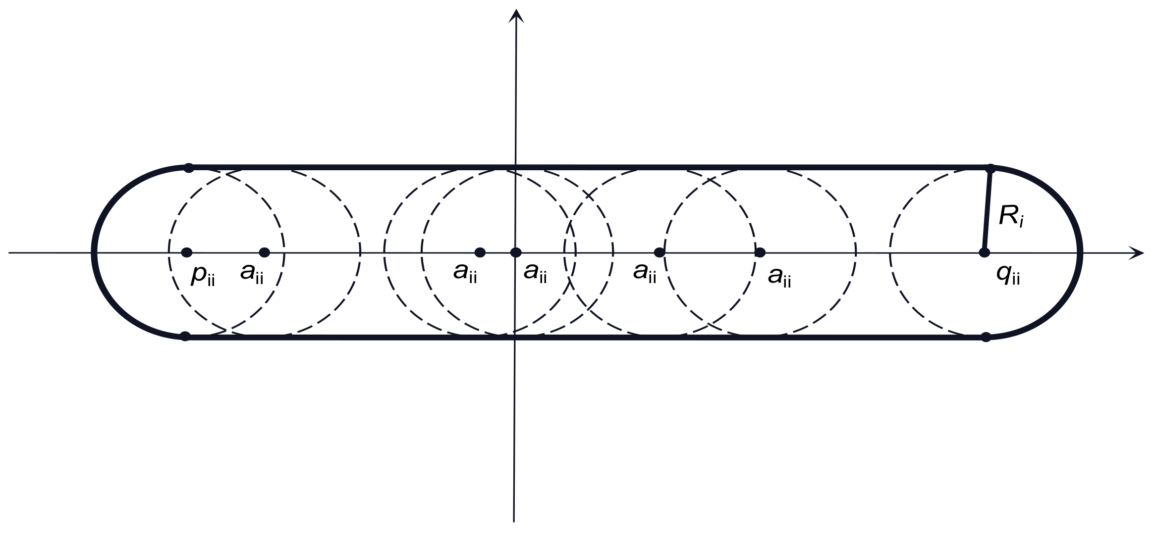
Proof. Applying the Geršgorin disc theorem, for any
, every
must lie in at least one of n closed discs, i.e.,
As
locates on the x axis, so we can obtain n small discs centered at
and with radius
. There is an annulus runway which is symmetric with respect to the x axis containing all the n small discs. We can express the annulus runway as follows:
The significance of the above formula is shown in
Figure 1.
For an
interval matrix
, there are numerous annulus runways like
Figure 1, containing all the eigenvalues of interval matrix
, so we can use a single big annulus runway containing all the small annulus runways. We can express the big annulus runway as follows:
The significance of the above formula is shown in
Figure 2.
Thus, , and the proof is completed. □
If all the elements of an interval matrix belong to the same interval, then an application of Theorem 1 can be seen in the following result.
Corollary 1. Let be an interval matrix and be the set of eigenvalues of :where is the maximum of . Then, .
3. The Spread of Interval Matrices
In this section, we give some upper bounds of the spread of general interval matrices and real symmetric interval matrices.
Based on Theorem 1, we have our first result for upper bounds of the spread of general interval matrices.
Theorem 2. Let be an interval matrix and the set of eigenvalues of : . Then, Proof. In Theorem 1, we bind all eigenvalues of a given interval matrix in a single big annulus runway in the complex plane; then, the spread of
must not exceed the major axis
in the annulus runway, that is
must not exceed the minor axis
in the annulus runway, that is
The proof is completed. □
In order to obtain a better upper bound for the spread of interval matrices, we introduce a lemma from reference [
13].
Lemma 2. Let be any complex numbers, and writethen,with equality if and only if satisfy condition φ. Remark 1. If n complex numbers are such that among them are equal to each other and to the arithmetic mean of the remaining two, we shall say that the n numbers satisfy condition φ.
Based on inequality (
2) in Lemma 2, we have another result about the upper bound for the spread of interval matrices.
Theorem 3. Let be an interval matrix and be the set of eigenvalues of ; then, Proof. According to inequality (
2), for any matrix
, we can obtain
for the eigenvalues
of matrix
A. By Lagrange’s identity, it follows that
thus,
and then,
By the following inequality in [
19],
then, we have
Apply inequalities (
4) and (
5) to (
3), and we can obtain the following conclusion:
The above inequality holds for any matrix . The proof is completed. □
Remark 2. The upper bound of spread of Theorem 3 is more accurate than the result of Theorem 2.
Next, we will consider a special type of interval matrices whose entries are in the interval . The following lemma about an equality for the variance of a discrete random variable is necessary.
Lemma 3. ([
20], Lemma 1).
Let be discrete random variables, and then, Based on inequality (
3) and Lemma 3, we have the following theorem.
Theorem 4. Let and ; then, Proof. By inequality (
3) and
, we have
Since the elements of A locate in the interval
,
cannot attain the maximum until
attains the maximum. Without loss of generality, we have the following inequality:
So taking
as the maximum of
we obtain
By the variance formula, then we have
Combining (
7) with Lemma 3, then
cannot achieve the maximum until
attains the maximum and
attains the minimum simultaneously.
If
n is even, let
that is
or
Now, we can consider
as a function
and
can achieve the maximum as
and
or
Let
; then,
solving the equation
, so we conclude that
Combining (
6) with (
8), we have
If
n is odd, let
, that is
or
. Similar to
n being even,
so we conclude that
, and then,
Combining (
6) with (
9), we have
The proof is completed. □
Corollary 2. Let and ; then, Remark 3. If n is even, the conclusion in Corollary 2 is the same as inequality (1), but we have provided a more concise proof. 4. Numerical Example
In this section, we will give several examples to illustrate the effectiveness of our results.
Example 1. In interval matrix , we have .
Choose a matrix , The eigenvalues of A areso we obtain From Theorem 1, we can obtain the following region: Clearly, we can obtain
From Theorem 3, we havewhich provides a more precise estimation for the spread of interval matrices than Theorem 2. Example 2. Choose a matrix , The eigenvalues of B are then, we have From Corollary 1, we obtain the following region: Clearly, we can obtain
From Theorem 4, we haveand the upper bounds of the spread is more precise than Theorems 2 and 3. Example 3. Choose a matrix and , The eigenvalues of C are then, we haveand the eigenvalues of D are From Corollary 2, we have
5. Conclusions
We present the distribution of eigenvalues of interval matrices and establish upper bounds for their spread. Theorem 1 provide the distribution of eigenvalues of interval matrices. Theorems 2 and 3 both offer upper bounds for the spread of general interval matrices. Notably, the upper bound provided by Theorem 4 exhibits higher accuracy compared with that of Theorems 2 and 3. Theorem 4 introduces upper bounds for the spread of symmetric interval matrices, and we obtain the same inequality as (
1) when
n is even based on a simple proof.
Author Contributions
This work was carried out in collaboration between the authors. P.L. designed the study and guided the research. W.L. performed the analysis and wrote the first draft of the manuscript. P.L. and W.L. managed the analysis of the study. All authors have read and agreed to the published version of the manuscript.
Funding
This research was supported by the Science and Technology Research Program of Chongqing Municipal Education Commission (grant No. KJQN201901546 and No. KJQN201901518) and the Science and Technology Research Program of Chongqing Municipal Education Commission (grant No. KJQN202101536).
Institutional Review Board Statement
We certify that this manuscript is original and has not been published and will not be submitted elsewhere for publication while being considered by Mathematics. And, the study is not split up into several parts to increase the number of submissions and submitted to various journals or to one journal over time.
Data Availability Statement
Data sharing not applicable.
Acknowledgments
All authors are thankful to the honorable reviewers for their valuable suggestions and comments, which improved the paper.
Conflicts of Interest
The authors declare no conflict of interest.
References
- Wu, J.L.; Zhang, P.P.; Liao, W.S. Upper bounds for the spread of a matrix. Linear Algebra Appl. 2012, 437, 2813–2822. [Google Scholar] [CrossRef]
- Wu, J.L.; Zhang, P.P.; Wang, Y. The location for eigenvalues of complex matrices by a numerical method. J. Appl. Math. Inform. 2011, 29, 49–53. [Google Scholar]
- Leng, H.N.; He, Z.Q. Eigenvalue bounds for symmetric matrices with entries in one interval. Appl. Math. Comput. 2017, 299, 58–65. [Google Scholar] [CrossRef]
- Milan, H.; Daney, D.; Tsigaridas, E. Characterizing and approximating eigenvalue sets of symmetric interval matrices. Comput. Math. Appl. 2011, 62, 3152–3163. [Google Scholar]
- Milan, H. Bounds on eigenvalues of real and complex interval matrices. Appl. Math. Comput. 2013, 219, 5584–5591. [Google Scholar]
- Falguni, R.; Gupta, D.K. Sufficient regularity conditions for complex interval matrices and approximations of eigenvalues sets. Appl. Math. Comput. 2018, 317, 193–209. [Google Scholar]
- Firouzbahrami, M.; Babazadeh, M.; Nobakhti, A.; Karimi, H. Improved bounds for the spectrum of interval matrices. IET Control. Theory Appl. 2013, 7, 1022–1028. [Google Scholar] [CrossRef]
- Sukhjit, S.; Gupta, D.K. Eigenvalues bounds for symmetric interval matrices. Int. J. Comput. Sci. Math. 2015, 6, 311–322. [Google Scholar]
- Wu, J.L. Upper (lower) bounds of the eigenvalues, spread and the open problems for the real symmetric interval matrices. Math. Methods Appl. Sci. 2013, 36, 413–421. [Google Scholar] [CrossRef]
- Milan, H. Complexity issues for the symmetric interval eigenvalue problem. Open Math. 2015, 13, 157–164. [Google Scholar]
- Zhan, X. Extremal eigenvalues of real symmetric matrices with entries in an interval. SIAM J. Matrix Anal. Appl. 2006, 27, 850–851. [Google Scholar] [CrossRef]
- Moore, R.E. Interval Analysis; NJ-Prentice Hall: Englewood and Cliffs, NJ, USA, 1966. [Google Scholar]
- Mirsky, L. The spread of a matrix. Mathematika 1956, 3, 127–130. [Google Scholar] [CrossRef]
- Mirsky, L. Inequalities for normal and Hermitian matrices. Duke Math. J. 1957, 24, 591–599. [Google Scholar] [CrossRef]
- Deutsch, E. On the spread of matrices and polynomials. Linear Algebra Appl. 1978, 22, 49–55. [Google Scholar] [CrossRef]
- Beesack, P.R. The spread of matrices and polynomials. Linear Algebra Appl. 1980, 31, 145–149. [Google Scholar] [CrossRef]
- Tu, B.X. On the spread of a matrix. J. Fudan Univ. (Nat. Sci.) 1984, 23, 435–441. [Google Scholar]
- Horn, R.A.; Johnson, C.R. Matrix Analysis; Cambridge University Press: Cambridge, UK, 1985. [Google Scholar]
- Schur, I. Über die charakteristischen Wurzeln einer linearen substitution mit einer Anwendung auf die Theorie der Integralgleichungen. Math. Ann. 1909, 66, 488–510. [Google Scholar] [CrossRef]
- Moors, J.J.A.; Muilwijk, J. An inequality for the variance of a discrete random variable. Indian J. Stat. Ser. B 1971, 33, 385–388. [Google Scholar]
| Disclaimer/Publisher’s Note: The statements, opinions and data contained in all publications are solely those of the individual author(s) and contributor(s) and not of MDPI and/or the editor(s). MDPI and/or the editor(s) disclaim responsibility for any injury to people or property resulting from any ideas, methods, instructions or products referred to in the content. |
© 2023 by the authors. Licensee MDPI, Basel, Switzerland. This article is an open access article distributed under the terms and conditions of the Creative Commons Attribution (CC BY) license (https://creativecommons.org/licenses/by/4.0/).


