Predator–Prey Model Considering Implicit Marine Reserved Area and Linear Function of Critical Biomass Level

Abstract

In this work, we examine a predator–prey model that considers the implicit marine reserve in prey species and a linear function of critical biomass level. The model’s basic properties (existence, uniqueness, positivity, boundedness, and permanence) and equilibrium points are determined. We obtain three equilibrium points: the trivial equilibrium point, the equilibrium point where there is no harvest, and the co-existing equilibrium point. The local and global stability of each equilibrium point of the model is explored. Moreover, the interior equilibrium point is always globally asymptotically stable, and the system experiences no limit cycles around the interior equilibrium point. Numerical simulations are conducted to illustrate the theoretical results obtained. Finally, we find overlapping conditions regarding the dynamics between the model we developed and a model that considers a constant critical biomass level for certain parameters.

1. Introduction

The predator–prey interaction is one of the interactions that occurs in ecological problems. This interaction has been researched for decades by mathematicians who invest their time in creating accurate and useful models. The predator–prey model was first introduced independently by Alfred J. Lotka in 1925 and Vito Volterra in 1926 [1]. The Lotka–Volterra predator–prey system for two species is modeled as follows:

$$\left\{\begin{array}{c}\frac{dx}{dt}=gx-pxy\\ \frac{dy}{dt}=nxy-dy\end{array}.\right.$$

In the Lotka–Volterra predator–prey model, the variables $x$ and $y$ represent the prey and predator population densities, respectively. The intrinsic growth rate of the prey is represented by $g$. The predation rate of the predator on the prey is represented by $p$. The growth of the predator is assumed to be influenced only by the predation effect, with a growth rate represented by $n$. Finally, the parameter $d$ is the natural mortality rate of the predator.

To incorporate the human effect into a natural growth of a population, researchers then introduced the harvesting effect into the growth model in various ways. As an example, in 1957, Schaefer [2] introduced a harvesting model in a simple fisheries ecosystem without considering predation. Harvesting is expressed as a function $qEx$, where $q$ and $E$ represent catchability coefficient and harvesting effort, respectively. The Schaefer [2] model was developed as a management tool for the Eastern Tropical Pacific Tuna Fishery [3]. The Schaefer [2] fishery model is presented as follows:

$$\left\{\frac{dx}{dt}=gx\left(1-\frac{x}{K}\right)-qEx.\right.$$

The Schaefer model [2] consists of only one equation with only one variable. The variable can be represented as either predator or prey. The parameter $K$ represents the tuna population’s carrying capacity. Besides the harvesting function in Schaefer [2], there are also other harvesting functions, including the constant harvesting function [4,5], the rational harvesting function [6,7,8], the periodic harvesting function [9,10,11], and the piecewise harvesting function [11,12].

Since real problems are more complex than those modeled by the Lotka–Volterra and Schaefer models, the two models have been widely combined and developed to get realistic modeling or at least one that is close to the real problem. Meng et al. [13] combined the two models by considering a disease in a species so that the prey species consisted of susceptible and infected preys. Thirthar et al. [14] studied three species of prey, predator, and superpredator species and added the effect of fear between predators and prey. They showed in their analysis that fear has a noticeable effect on the system’s stability. Suryanto et al. [15] studied the fractional derivative Caputo model with a ratio-dependent predation function. The fractional model was formed by them because the population growth rate depends on long-term memory. Panigoro et al. [16] studied the fractional derivative Caputo predator–prey model and harvesting by considering the age structure of predators consisting of juvenile and adult predators. They assumed that only adult predators can prey on preys.

In recent years, the development of research on predator–prey mathematical models and harvesting by mathematicians has extended to marine reserves (can be seen in [17]). Mapunda et al. [18] studied the predator–prey system by considering the creation of a marine reserve as a solution to over-exploitation and drought in the system. Based on their results, when the creation of marine reserves is not performed, it will have a negative impact on the predator and prey populations. Abid et al. [19] analyzed the stability and determined the optimal harvesting of the modified Leslie–Gower predator–prey model by considering the implicit marine reserve. Ibrahim [20] proposed a predator–prey model that considers the implicit marine reserve and critical biomass level with the harvesting function following the harvesting function in [2,21], namely

$$h\left(x,E\right)=qEx,$$

(1)

where $q$, $E$, and $x$ are the catchability coefficient, constant harvesting effort, and prey population density. Furthermore, the research model from Ibrahim [20] is presented as follows:

$$\left\{\begin{array}{c}\frac{dx}{dt}=rx\left(1-\frac{x}{K}\right)-uqEx\\ \frac{dE}{dt}=uqE\left(x-a\right)\end{array}\right.,$$

(2)

Based on the model in (2), Ibrahim [20] assumed that changes in population density increase with prey population growth and decrease with prey harvesting. Prey population growth is described by a logistic function, $rx(1-\frac{x}{K})$, with $K$ and $r$ being the prey’s carrying capacity and intrinsic growth rate, respectively. Then, prey harvesting is described by the function in (1), with $u$ being the implicit marine reserve fraction, i.e., the fraction of prey stock allowed to be harvested. Therefore, $(1-u)$ is the fraction of prey stock that is not allowed to be harvested. Furthermore, the change in fishing effort can increase or decrease depending on the value of $(x-a)$, where $a\in (0,K)$ is the economically critical stock size level. The term $(x-a)$ has the interpretation that when the prey population density $\left(x\right)$ is greater than the threshold $a$ ($x>a$), the effort ($E$) in harvesting the prey population increases. When the prey population density is smaller than threshold $a$, harvesting effort ($E$) decreases. In this condition, if $E$ is still increased, the fishermen will not get profit (loss). Finally, when $x=a$, the effort in harvesting does not change (constant).

In this study, we modify the model in [20] by replacing the term $(x-a)$ with $(x-aE)$. The modified model is presented as follows:

$$\frac{dU}{dt}=\left[\begin{array}{c}\frac{dx}{dt}\\ \frac{dE}{dt}\end{array}\right]=\left[\begin{array}{c}rx\left(1-\frac{x}{K}\right)-uqEx\\ uqE\left(x-aE\right)\end{array}\right]=\left[\begin{array}{c}{H}_1\left(U\right)\\ H_2\left(U\right)\end{array}\right]=H(U),$$

(3)

Based on the economic system prevailing in most regions, fishermen will flock there when the fishery shows success. As a result, the fishing rate increases and the fish population catches up [21]. Therefore, the amount of fishing effort made by fishermen also greatly affects the rise and fall of the fishing rate. Based on the term $(x-aE)$, the harvesting effort on prey increases when $\frac{x}{E}>a$, which is the ratio of prey population density to fishing effort greater than $a$. Then, when $\frac{x}{E}<a$, the harvesting effort on the prey decreases. This means that some fishermen choose to move to other waters because fishermen can experience losses if they continue harvesting in these waters. Finally, when $\frac{x}{E}=a$, the harvesting effort does not change.

This study aims to explore the solution properties of the model developed in (3). The exploration of the solution properties of the model in (3) is presented in Section 2. Then, this study determines the equilibrium points of the model in (3) and analyzes their local stability, which is presented in Section 3 and Section 4, respectively. In Section 5 and Section 6, the asymptotic global stability and existence of limit cycles are analyzed. The bionomic equilibrium point is determined and discussed in Section 7. In Section 8, numerical simulations are performed to demonstrate the results obtained graphically. Next, Section 9 aims to discuss or show that there are overlapping conditions between the model we developed and the model developed by Ibrahim [20]. These conditions are obtained by selecting certain parameters. Finally, the conclusion of this study is presented in Section 10.

2. Basic Properties of the Model Solution

In this section, we present some basic properties of the solution of the model in (3). The properties that will be discussed include existence and uniqueness, positivity, boundedness, and permanence. The solution properties ensure that the model has a unique solution and that the solution is related to the biological problem.

2.1. Existence and Uniqueness of Solutions

Lemma 1 

(Picard–Lindelöf theorem in [22]). If the function $f:A\to {\mathbb{R}}^n$ is continuous and locally Lipschitz in $x$ in an open set $A\subset \mathbb{R}\times {\mathbb{R}}^n$, then for every $\left(t_0,x_0\right)\in A$ there exists a unique solution of the initial value problem

$$\frac{dx}{dt}=f\left(x\left(t\right)\right), x\left(t_0\right)=x_0.$$

in some open interval containing $t_0$.

Lemma 1 is used to show the existence and uniqueness of the solution of the model in (3) which is presented in the following Theorem.

Theorem 1. 

$H\left(U\right)$ in (3) is Lipschitz-continuous, so (3) has a unique solution, namely $x\left(t\right)$ and $E\left(t\right)$ in ${\mathsf{\Omega }}_M=\left\{{\left[x, E\right]}^T\in {\mathbb{R}}_{+}^2|\mathit{max}\left\{\left|x\right|,\left|E\right|\le M\right\}\right\}$ for $t\ge 0$.

Proof of Theorem 1. 

First, it is clear that $H_1\left(U\right)$ and $H_2\left(U\right)$ of $H\left(U\right)$ in (3) are continuous functions. Second, we will show that $H\left(U\right)$ is a Lipschitz function in the region $\left[0,\infty \right)\times {\mathsf{\Omega }}_M$. In this case, the solution of the model in (3) is assumed to be bounded in $M$, whose boundedness is shown in Theorem A2. Suppose $U={\left[x,E\right]}^T, \overline{U}={\left[\overline{x}, \overline{E}\right]}^T$, and mapping

$$H\left(U\right)=\left[\begin{array}{c}{H}_1\left(U\right)\\ H_2\left(U\right)\end{array}\right],$$

(4)

where

$$\begin{array}{c}{H}_1\left(U\right)=rx\left(1-\frac{x}{K}\right)-uqEx\\ H_2\left(U\right)=uqE\left(x-aE\right).\end{array}$$

(5)

For any $U, \overline{U}\in {\mathsf{\Omega }}_M$, we have that

$$\begin{array}{ll}‖H\left(U\right)-H\left(\overline{U}\right)‖& =\left|H_1\left(U\right)-H_1\left(\overline{U}\right)\right|+\left|H_2\left(U\right)-H_2\left(\overline{U}\right)\right|\\ & =\left|rx\left(1-\frac{x}{K}\right)-uqEx-r\overline{x}\left(1-\frac{\overline{x}}{K}\right)+uq\overline{E}\overline{x}\right|\\ & +\left|uqEx-uq{E}^{2}a-uq\overline{E}\overline{x}+uq{\overline{E}}^{2}a\right|\\ & =\left|r\left(x-\overline{x}\right)+\frac{r}{K}\left(-x^2+{\overline{x}}^2\right)+uq\left(-Ex+\overline{E}\overline{x}\right)\right|\\ & +\left|uq\left(Ex-\overline{E}\overline{x}\right)+uqa\left(-E^2+{\overline{E}}^2\right)\right|\\ & \le r\left|x-\overline{x}\right|+\frac{r}{K}\left|-x^2+{\overline{x}}^2\right|+uq\left|-Ex+\overline{E}\overline{x}\right|+uq\left|Ex-\overline{E}\overline{x}\right|\\ & +uqa\left|-E^2+{\overline{E}}^2\right|\\ & =r\left|x-\overline{x}\right|+\frac{r}{K}\left|x+\overline{x}\right|\left|x-\overline{x}\right|+2uq\left|Ex-\overline{E}\overline{x}\right|+uqa|E+\overline{E}||E-\overline{E}|\\ & \le \left(r+\frac{2r}{K}M+2uqM\right)\left|x-\overline{x}\right|+\left(2uqM+2uqaM\right)\left|E-\overline{E}\right| \\ & \le L‖U-\overline{U}‖,\end{array}$$

(6)

where $L=\max \left\{\left(r+\frac{2r}{K}M+2uqM\right),\left(2uqM+2uqaM\right)\right\}$. Based on this, there exists $L$ such that $‖H\left(U\right)-H\left(\overline{U}\right)‖\le L‖U-\overline{U}‖$. Consequently, $H\left(U\right)$ satisfies the Lipschitz condition on $U$. Hence, $H\left(U\right)$ is a Lipschitz-continuous function. Furthermore, by Lemma 1, the model in (3) has unique solutions $x\left(t\right)$ and $E\left(t\right)$ on ${\mathsf{\Omega }}_M$. □

2.2. Permanence of Solutions

Definition 1 

([23]). A system of equations, namely $\frac{dx}{dt}=f(x,y)$ and $\frac{dy}{dt}=g(x,y)$, is said to be permanent if there are constants $m$ and $M$ $(0<m<M)$ such that the positive solution of the system ($x\left(t\right)$ and $y\left(t\right)$) with respect to the initial values $\left(x\left(0\right),y\left(0\right)>0\right)$ satisfies the condition of

$$\begin{gathered} \min \{\underset{t\to +\infty }{\lim }\inf x\left(t\right), \underset{t\to +\infty }{\lim }\inf y\left(t\right)\}\ge m, \\ \max \{\underset{t\to +\infty }{\lim }\sup x\left(t\right), \underset{t\to +\infty }{\lim }\sup y\left(t\right)\}\le M, \end{gathered}$$

(7)

Lemma 2 

([24] in [23]). For ${\tau }_1,{\tau }_2>0$, $x\left(0\right)>0$, and

1. 

$\frac{dx}{dt}\le x({\tau }_1-{\tau }_{2}x)$, then$\underset{t\to +\infty }{\lim }\sup x\left(t\right)\le \frac{{\tau }_1}{{\tau }_2}$;

2. 

$\frac{dx}{dt}\ge x({\tau }_1-{\tau }_{2}x)$, then $\underset{t\to +\mathrm{\infty }}{\lim }\inf x\left(t\right)\ge \frac{{\tau }_1}{{\tau }_2}$.

Theorem 2. 

If $r>\frac{uqK}{a}$, then the solution of the model in (3), i.e., $x\left(t\right)$ and $E\left(t\right)$ for each $t\ge 0$, is a permanent solution by satisfying the initial values $x\left(0\right)>0$ and $E\left(0\right)>0$.

Proof of Theorem 2. 

We first claim that the solution of the model in (3) is a bounded solution. The proof of this claim is presented in Appendix A. Based on the boundedness of the solutions of the model in (3) proven in Appendix A, we get

$$\underset{t\to +\infty }{\lim }\sup x\left(t\right)\le K \mathrm{and} \underset{t\to +\infty }{\lim }\sup E\left(t\right)\le \frac{K}{a}.$$

Therefore, for a sufficiently small $\epsilon >0$, there exists $T>0$ such that

$$x\left(t\right)\le K+\epsilon \mathrm{and} E\left(t\right)\le \frac{K}{a}+\epsilon \mathrm{for} t>T.$$

As a result,

$$\frac{dx}{dt}=x\left(\left(r-\frac{rx}{K}\right)-uqE\right)\ge x\left(r-uq\left(\frac{K}{a}+\epsilon \right)-\frac{r}{K}x\right).$$

Based on Lemma 2 with ${\tau }_1=r-uq\left(\frac{K}{a}+\epsilon \right)$ and ${\tau }_2=\frac{r}{K}$, when ${\tau }_1>0$, we obtain

$$\underset{t\to +\infty }{\lim }\inf x\left(t\right)\ge \frac{r-uq\left(\frac{K}{a}+\epsilon \right)}{\frac{r}{K}}=\frac{K\left(r-uq\left(\frac{K}{a}+\epsilon \right)\right)}{r}.$$

Therefore, for $\epsilon \to 0$, we obtain

$$\underset{t\to +\infty }{\lim }\inf x\left(t\right)\ge \frac{K\left(r-uq\frac{K}{a}\right)}{r}={\omega }_1.$$

Thus, ${\omega }_1>0$ if $r>\frac{uqK}{a}$.

Using the same steps with ${\tau }_1=uqK$ and ${\tau }_2=uqa$, we obtain

$$\underset{t\to +\infty }{\lim }\inf E\left(t\right)\ge \frac{uqK}{uqa}=\frac{K}{a}={\omega }_2>0.$$

Thus, $x\left(t\right)$ and $E\left(t\right)$ are permanent solutions for each $t\ge 0$ to the initial conditions $x\left(0\right)>0$ and $E\left(0\right)>0$ if values $m=\min \{{\omega }_1,{\omega }_2\}$ and $M=\max \{K,\frac{K}{a}\}$. □

3. Equilibrium Points and Their Existence

The equilibrium points can be determined by making the terms $\frac{dx}{dt}$ and $\frac{dE}{dt}$ of Equation (3) equal zero, i.e., $\frac{dx}{dt}=\frac{dE}{dt}=0$. By finding the solution of $\frac{dx}{dt}=\frac{dE}{dt}=0$, there are three equilibrium points, namely

• The trivial (origin) equilibrium point $P_0={\left[x_0,E_0\right]}^T={\left[\mathrm{0,0}\right]}^T$ which always exists;
• The effort harvesting extinction equilibrium point $P_1={\left[x_1,E_1\right]}^T={\left[K,0\right]}^T$ which always exists;
• The co-existence (interior) equilibrium point $P_2={\left[x_2,E_2\right]}^T={\left[a{E}_2,\frac{rK}{Kqu+ar}\right]}^T$ which always exists.

4. Local Stability of Each Equilibrium Point

The local stability of each equilibrium point for system (3) is explored with the help of its Jacobian matrix. If the real parts of all eigenvalues of the Jacobian matrix for each equilibrium point are nonpositive, then system (3) is locally stable toward the corresponding equilibrium point. Conversely, if the real part of any eigenvalue is positive, system (3) is not locally stable at the corresponding equilibrium point. Suppose the eigenvalues of the Jacobian matrix of an equilibrium point cannot be obtained explicitly. In that case, the help of the Routh–Hurwitz criterion is needed in determining the local stability of the equilibrium point. The local stability of the equilibrium points $P_0$, $P_1$, and $P_2$ are presented in Theorem 3, Theorem 4, and Theorem 5, respectively.

Theorem 3. 

For the model in (3), the equilibrium point $P_0$ is always a saddle.

Proof of Theorem 3. 

For equilibrium point $P_0$, the Jacobian matrix is

$$J\left(P_0\right)=J\left(x_0, E_0\right)=\left[\begin{array}{cc}r& 0\\ 0& 0\end{array}\right].$$

Furthermore, the eigenvalues obtained from the matrix $J\left(P_0\right)$ are ${\lambda }_1=r>0$ and ${\lambda }_2=0$. Since ${\lambda }_1>0$, the equilibrium point $P_0$ is always a saddle. □

Theorem 4. 

For the model in (3), the equilibrium point $P_1$ is always a saddle.

Proof of Theorem 4. 

For equilibrium point $P_1$, the Jacobian matrix is

$$J\left(P_1\right)=J\left(x_1, E_1\right)=\left[\begin{array}{cc}-r& -Kqu\\ 0& Kqu\end{array}\right].$$

Furthermore, the eigenvalues obtained from the matrix $J\left(P_1\right)$ are ${\lambda }_1=-r<0$ and ${\lambda }_2=Kqu>0$. Based on these two eigenvalues, the equilibrium point $P_1$ is a saddle. □

Theorem 5. 

For the model in (3), the equilibrium point $P_2$ is always asymptotically locally stable. Furthermore, the equilibrium point $P_2$ yields the following

1. 

Semi-spiral sink or star sink, if ${\left(uqK-r\right)}^{2}a>4{\left(uqK\right)}^2$;

2. 

Sink, if ${\left(uqK-r\right)}^{2}a=4{\left(uqK\right)}^2$;

3. 

Spiral sink, if ${\left(uqK-r\right)}^{2}a<4{\left(uqK\right)}^2$.

Proof of Theorem 5. 

Evaluation of the Jacobian matrix at equilibrium point $P_2$, namely

$$J\left(P_2\right)=J\left(x_2, E_2\right)=\left[\begin{array}{cc}\frac{rK-\left(uqK+2ar\right)E_2}{K}& -uqa{E}_2\\ uq{E}_2& -uqa{E}_2\end{array}\right].$$

Then,

$$trace\left(J\left(P_2\right)\right)=-\frac{ar\left(uqK+r\right)}{uqK+ar}<0 \mathrm{and} \det \left(J\left(P_2\right)\right)=\frac{aKq{r}^{2}u}{uqK+ar}>0.$$

Therefore, the equilibrium point $P_2$ is locally asymptotically stable. Furthermore, the value of

$$\det \left(J\left(P_2\right)\right)-\frac{{\left(trace\left(J\left(P_2\right)\right)\right)}^2}{4}=-a{r}^2\left({\left(uqK-r\right)}^{2}a-4{\left(Kqu\right)}^2\right).$$

(8)

Equation (8) is zero if ${\left(uqK-r\right)}^{2}a=4{\left(uqK\right)}^2$. Therefore, if Equation (8) is zero, the equilibrium point $P_2$ produces a semi-spiral sink or star sink. Then, Equation (8) is less than zero if ${\left(uqK-r\right)}^{2}a>4{\left(uqK\right)}^2$. Therefore, if Equation (8) is less than zero, the equilibrium point $P_2$ generates a sink. Finally, Equation (8) is greater than zero if ${\left(uqK-r\right)}^{2}a<4{\left(uqK\right)}^2$. Therefore, if Equation (6) is greater than zero, the equilibrium point $P_2$ produces a spiral sink. □

5. Global Stability of Equilibrium Point ${\mathit{P}}_{\mathbf{2}}$

Based on the local stability analysis of each equilibrium point of the model in Equation (3), there is only one stable equilibrium point, namely equilibrium point $P_2$. Therefore, the global stability analysis is only carried out at equilibrium point $P_2$. The stability can be determined using the Lyapunov method or theorem. This method starts by determining a positive definite function. The global stability of $P_2$ is presented in Theorem 6.

Theorem 6. 

The equilibrium point $P_2$ of the model in (3) is globally asymptotically stable $\forall (x_0,E_0)>0$

Proof of Theorem 6. 

A positive definite function of the model in (3) is presented as follows:

$$V=\left(x-x^{*}-x^{*}\ln \frac{x}{x^{*}}\right)+\left(E-E^{*}-E^{*}\ln \frac{E}{E^{*}}\right).$$

The derivative of the function $V$ with respect to time $t$ is given by

$$\frac{dV}{dt}=\left(1-\frac{x^{*}}{x}\right)\frac{dx}{dt}+\left(1-\frac{E^{*}}{E}\right)\frac{dE}{dt}.$$

Then, based on the model in (3),

$$\frac{dV}{dt}=\left(x-x^{*}\right)\left[r\left(1-\frac{x}{K}\right)-uqE\right]+uq\left(x-aE\right)\left(E-E^{*}\right).$$

At equilibrium point $P_2$ (interior equilibrium),

$$\begin{gathered} r\left(1-\frac{x^{*}}{K}\right)-uq{E}^{*}=0\to r=uq{E}^{*}+\frac{r{x}^{*}}{K}, \\ {x}^{*}=a{E}^{*}. \end{gathered}$$

Thus,

$$\begin{array}{ll}\frac{dV}{dt}& =\left(x-x^{*}\right)\left[r-\frac{rx}{K}-uqE\right]+uq\left(E-E^{*}\right)\left(x-aE\right)\\ & =\left(x-x^{*}\right)\left[uq{E}^{*}+\frac{r{x}^{*}}{K}-\frac{rx}{K}-uqE\right]+uq\left(E-E^{*}\right)\left(x-aE\right)\\ & =\left(x-x^{*}\right)\left[-\frac{r\left(x-x^{*}\right)}{K}-uq\left(E-E^{*}\right)\right]+uq\left(E-E^{*}\right)\left(x-aE\right)\\ & =-\left(x-x^{*}\right)\left[\frac{r\left(x-x^{*}\right)}{K}+uq\left(E-E^{*}\right)\right]+uq\left(E-E^{*}\right)\left(x-aE\right)\\ & =-\frac{r}{K}{\left(x-x^{*}\right)}^2-uq\left(E-E^{*}\right)x+uq\left(E-E^{*}\right)x+uq\left(E-E^{*}\right)a{E}^{*}\\ & \hspace{1em}\hspace{1em}\hspace{1em}\hspace{1em}\hspace{1em}\hspace{1em}-uq\left(E-E^{*}\right)aE\\ & =-\frac{r}{K}{\left(x-x^{*}\right)}^2-auq{\left(E-E^{*}\right)}^2<0.\end{array}$$

Therefore, $\frac{dV}{dt}$ has a negative definite value. Consequently, the equilibrium point $P_2$ is globally asymptotically stable [25]. □

6. Limit Cycles

The following theorem indicates that system (3) does not possess any closed trajectories (or limit cycles) in the interior of the positive quadrant of the $x$−$E$ plane.

Theorem 7. 

The model in (3) has no limit cycles around the equilibrium point $P_2$

.

Proof of Theorem 7. 

Let

$$D\left(x,E\right)=\frac{1}{xE}, H_1\left(x,E\right)=rx\left(1-\frac{x}{K}\right)-uqEx, H_2\left(x,E\right)=uqE\left(x-aE\right).$$

Based on the positivity of the model solution in (3), $D\left(x,E\right)>0$ in the interior of the positive quadrant. Then,

$$\begin{gathered} \mathsf{\Delta }\left(x,E\right)=\frac{\partial \left(hf\right)}{\partial x}+\frac{\partial \left(hg\right)}{\partial E}=\frac{\partial }{dx}\left[\frac{r}{E}\left(1-\frac{x}{K}\right)-uq\right]+\frac{\partial }{\partial E}\left[uq\left(1-\frac{aE}{x}\right)\right] \\ =-\frac{r}{EK}-\frac{a}{x}<0. \end{gathered}$$

Since $\mathsf{\Delta }\left(x, E\right)$ does not change the sign in the positive quadrant, based on the Bendixson–Dulac criterion, consequently, the model in (3) has no limit cycles [26,27]. □

7. Bionomic Equilibrium

Bionomic equilibrium is a condition where the total revenue from harvested biomass sales equals the total cost incurred in harvesting fish. Let $c$ and $p$ represent the harvesting cost per unit effort and the selling price per unit biomass of landed fish, respectively. The net economic revenue at time $t$ is expressed as follows:

$$\pi \left(x,E,t\right)=\left(puqx-c\right)E.$$

(9)

Based on (9) and (3), bioeconomic equilibrium can be determined by finding the solution

$$\frac{dx}{dt}=\frac{dE}{dt}=\pi =0.$$

This means,

$$r\left(1-\frac{x}{K}\right)-uqE=0, uqE\left(x-aE\right)=0, \left(puqx-c\right)E=0.$$

(10)

Based on Equation (10), when $c>puqx$, the profit obtained will be negative (loss). Therefore, profit (existence of bionomic equilibrium) is obtained when $puqx>c$ [22]. Suppose $P_{\infty } (x_{\infty },E_{\infty },u_{\infty })$ represents the bionomic equilibrium point. Based on Equation (10), the bioeconomic equilibrium point is given by $x_{\infty }=a{E}_{\infty }$, $E_{\infty }=\frac{K}{ra}\left(r-\frac{c}{ap}\right)$, and $u_{\infty }=\frac{c}{pq{x}_{\infty }}$. It is clear that $E_{\infty }>0$ if $rap>c$.

Managers in the fisheries sector must be able to balance the commercial interests of fishermen and the sustainability of fisheries’ natural resources. Fishermen will suffer huge losses when the marine reserve area is too large. On the other hand, the sustainability of natural resources may not be achieved when the marine reserve is too small. Therefore, managers in the fisheries sector need to be careful in dividing the percentage of the area between marine reserve and unreserved areas. This can be done by considering the percentage of marine reserve area not approaching the bionomic equilibrium point. For example, when $u>u_{\infty }=\frac{c}{pq{x}_{\infty }}$, we obtain

$$\begin{array}{ll}\left(puqx-c\right)E& >\left(p{u}_{\infty }q{x}_{\infty }-c\right)E_{\infty }\\ & =\left(p\left(\frac{c}{pq{x}_{\infty }}\right)q{x}_{\infty }-c\right)E_{\infty }\\ & =\left(c-c\right)E_{\infty }=0.\end{array}$$

This result represents a positive economic rent. This condition attracts fishermen to enter this sector. On the other hand, if $u<u_{\infty }=\frac{c}{pq{x}_{\infty }}$, we obtain

$$\begin{array}{ll}\left(puqx-c\right)E& <\left(p{u}_{\infty }q{x}_{\infty }-c\right)E_{\infty }\\ & =\left(p\left(\frac{c}{pq{x}_{\infty }}\right)q{x}_{\infty }-c\right)E_{\infty }\\ & =\left(c-c\right)E_{\infty }=0.\end{array}$$

This result represents a negative economic rent so that fishermen leave the sector.

8. Numerical Simulations

This section presents numerical simulations of the results obtained in the previous sections. The software used for this numerical simulation was Maple 2019. All the codes are attached to the link listed in the Supplementary Materials section. Based on the results in Section 3, there are three equilibrium points, including (1) equilibrium point $P_0$ (trivial), which is the point where the element value of the equilibrium point is zero, meaning that the population density of prey species $\left(x\right)$ is extinct and there is no capture effort $\left(E\right)$; (2) equilibrium point $P_1$, which is the point where the population density of the prey $\left(x\right)$ is equal to $K$ while there is no capture effort $\left(E\right)$; (3) equilibrium point $P_2$, which is the point where the prey density $\left(x\right)$ and capture effort $(E$) exist. One of the three equilibrium points is always stable, namely equilibrium point $P_2$. Meanwhile, equilibrium points $P_0$ and $P_1$ are always saddle. Furthermore, equilibrium point $P_2$ is globally asymptotically stable, and system (3) has no limit cycle around equilibrium point $P_2$.

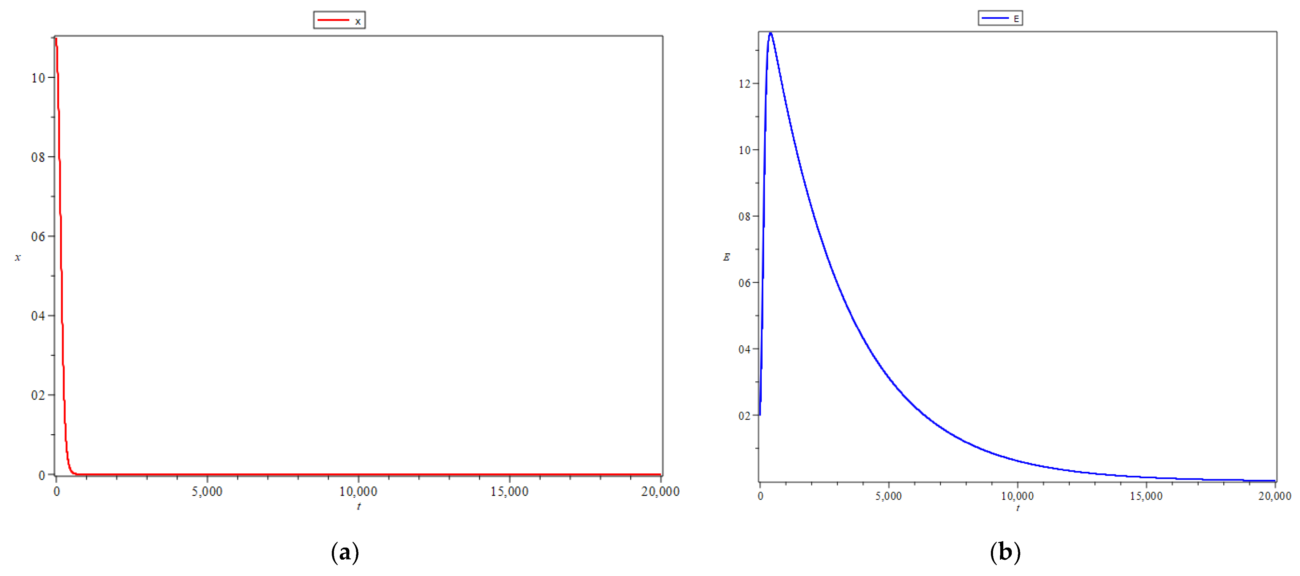
Numerical simulations were explored to show the local stability results of the three equilibrium points in Theorems 3, 4, and 5. The values of each parameter were $r=1.42$, $K=1000$, $u=0.6$, and $q=0.0018$. Meanwhile, the value of $a$ was varied based on the three conditions that satisfy Theorem 5. The value of $a$ is obtained from the result of $\frac{4{\left(uqK\right)}^2}{{\left(uqK-r\right)}^2}$, which is $40.35986159$. To fulfill the first, second, and third conditions of Theorem 6, parameter $a$ was greater than, equal to, and smaller than $40.35986159$ with values of $250$,$40.35986159$, and 0.025.

The numerical simulation result for $a=250$ is presented in Figure 1. This choice of parameter $a$ is intended to show that equilibrium point $P_2$ produces a semi-spiral sink or star sink. Figure 1 shows that all initial values of $x$ and $E$ in the positive quadrant will lead to equilibrium point $P_2={\left[x_2,E_2\right]}^T={\left[996.9669737, 3.987867895\right]}^T$. In Figure 1, the blue line represents more clearly that for some initial points ${\left[x\left(0\right),E\left(0\right)\right]}^T$, including

$$\left\{{\left[200,10\right]}^T,{\left[200,100\right]}^T,{\left[300,100\right]}^T,{\left[1800,100\right]}^T,{\left[2000,5\right]}^T, {\left[2000,100\right]}^T\right\}.$$

For $t\to \infty$, the points tend to equilibrium point $P_2.$

The numerical simulation result for $a=40.35986159$ is presented in Figure 2. The choice of parameter $a$ is intended to show that equilibrium point $P_2$ generates a sink. Figure 2 shows that all initial values of $x$ and $E$ in the positive quadrant will lead to equilibrium point $P_2={\left[x_2,E_2\right]}^T={\left[981.504, 24.31881481\right]}^T$. In Figure 2, the blue line represents more clearly that for some initial points ${\left[x\left(0\right),E\left(0\right)\right]}^T$, including

$$\left\{{\left[200,10\right]}^T,{\left[200,35\right]}^T,{\left[500,40\right]}^T,{\left[1000,40\right]}^T,{ \left[1500,5\right]}^T,{\left[1500,10\right]}^T,{\left[1500,20\right]}^T\right\}.$$

For $t\to \infty$, the points tend to equilibrium point $P_2.$

The numerical simulation result for $a=0.025$ is presented in Figure 3. The choice of parameter $a$ is intended to show that equilibrium point $P_2$ produces a spiral sink. Figure 3 shows that all initial values of $x$ and $E$ in the positive quadrant will lead to equilibrium point $P_2={\left[x_2,E_2\right]}^T={\left[31.82429404, 1272.971762\right]}^T$. In Figure 3, the blue line represents more clearly that for some initial points ${\left[x\left(0\right),E\left(0\right)\right]}^T$, including

$$\left\{{\left[80,1200\right]}^T,{\left[80,1300\right]}^T,{\left[90,1200\right]}^T,{\left[90,1500\right]}^T,{\left[120,1500\right]}^T,{\left[150,1800\right]}^T\right\},$$

For $t\to \infty$, the points tend to equilibrium point $P_2.$

Furthermore, Figure 1, Figure 2 and Figure 3 show that all initial values of $x$ and $E$ around equilibrium points $P_0={\left[0,0\right]}^T$, $P_1={\left[1000,0\right]}^T$, and $P_2$ converge to the corresponding equilibrium point $P_2$. It shows that the system around the equilibrium points $P_0$ and $P_1$ is always a saddle. Consequently, the equilibrium points are globally stable since they are valid for initial values in the positive quadrant. In addition, Figure 1, Figure 2 and Figure 3 also show that the equilibrium points are asymptotically globally stable, as shown by the absence of limit cycles.

9. Discussion

A predator–prey model considering implicit marine protected areas and critical biomass level was built and analyzed in this study. The model is presented in (3), which is a modification of the model from Ibrahim [20] in (2). Ibrahim [20], in his research, examined the boundedness of the solution of the model in (2). We also examined the boundedness of the solution of the model in (3). Furthermore, we examined the existence, uniqueness, and permanence of the solution of the model in (3), which was not studied by Ibrahim [20].

The next discussion in this paper is to determine the local and global stability of the equilibrium points of model (3). The determination of stability begins with the determination of the equilibrium point of model (3). Based on the results obtained in Section 3, there are three equilibrium points, namely $P_0$, $P_1$, and $P_2$. We found that the equilibrium points $P_0$ and $P_1$ of the models in (2) and (3) are the same: $P_0={\left[0,0\right]}^T$ and $P_1={\left[K,0\right]}^T$, respectively. However, the equilibrium point $P_2$ of the models in (2) and (3) can have the same and different values. The equilibrium point $P_2$ of model (2) is ${\left[x_2,E_2\right]}^T={\left[a,\frac{r}{uq}\left(1-\frac{a}{K}\right)\right]}^T$. Then, the equilibrium point $P_2$ of model (3) is ${\left[x_2,E_2\right]}^T={\left[a{E}_2,\frac{rK}{Kqu+ar}\right]}^T$. Furthermore, the equilibrium point $P_2$ of the model in (3) always exists. Meanwhile, the equilibrium point $P_2$ of the model in (2) will exist if $K>a$, which is stated in Ibrahim’s research [20]. The following remark presents the conditions under which the equilibrium points $P_2$ of models (2) and (3) are equal at $P_2={\left[a,1\right]}^T$.

Remark 1. 

The equilibrium point $P_2={\left[a,1\right]}^T$ of models (2) and (3) is the same if and only if $r\left(K-a\right)=uqK$.

Referring to Ibrahim’s research [20], the parameter values $u=0.6, q=0.0018, a=300$, and $K=1000.$ Based on Remark 1, we obtain $r=0.001542857143$. Therefore, the equilibrium point $P_2={\left[300,1\right]}^T$ is 300 tons of fish and one fishing trip. With these parameters, the numerical simulation results for models (2) and (3) are presented in Figure 4 and Figure 5, respectively. The steady state of model (3) is faster than the steady state of model (2) at $P_2$ with initial values of $x=400$ and $E=2$. In addition, we tried to change the value of $a$ to a smaller value, $a=0.3$. As a result, we obtained a value of $0.001080324097$. The simulation results for the new values of $a$ and $r$ are presented in Figure 6 and Figure 7. Figure 6 and Figure 7 show that the results for parameter $a=0.3$ are opposite to the results for parameter $a=300$. Figure 6 and Figure 7 show that the steady state of model (2) is faster than the steady state of model (3) at $P_2={\left[10,1\right]}^T$ with initial values $x=11$ and $E=2$.

After determining the equilibrium points of model (3), the next step was to determine the local and global stability of each of the equilibrium points. Based on our analysis, the local stability of $P_0$ and $P_1$ is always saddle, and $P_2$ is always asymptotically stable. This result is similar to the equilibrium points $P_0$ and $P_1$ of model (2), which are also always saddle, and $P_2$ is always asymptotically stable. In addition, equilibrium point $P_2$ is always globally stable, as proved using Lyapunov’s theorem. Furthermore, equilibrium point $P_2$ is globally asymptotically stable, and system (3) has no limit cycle around equilibrium point $P_2$. The results obtained are also similar to those of the equilibrium point $P_2$ of model (2) in that the equilibrium point is asymptotically globally stable.

Figure 4, Figure 5, Figure 6 and Figure 7 show that the same value of parameters for models (2) and (3) and $r\left(K-a\right)=uqK$ will result in the system stabilizing toward the same equilibrium point, which is at $P_2={\left[a,1\right]}^T$. The following theorem shows that different parameter values of models (2) and (3) can also result in a stable system at any equilibrium point $P_2$.

Theorem 8. 

For any parameters $r>0$, $K>0$, $0<u\le 1$, $0<q<1$, and $a>0$ of models (2) and (3) with equilibrium points $P_2$ of models (2) and (3), respectively, i.e., $P_2^{\left(2\right)}={\left[x_2^{\left(2\right)},E_2^{\left(2\right)}\right]}^T$ and $P_2^{\left(3\right)}={\left[x_2^{\left(3\right)}, E_2^{\left(3\right)}\right]}^T$. Let $r^{\left(i\right)}$, $K^{\left(i\right)}$, $u^{\left(i\right)}$, $q^{\left(i\right)}$, and $a^{\left(i\right)}$ be the parameters $r$, $K$, $u$, $q$, and $a$ of model (i) for $i=2, 3$. The two equilibrium points have the same values, namely$P_2={\left[x_2^{\left(2\right)},E_2^{\left(2\right)}\right]}^T={\left[x_2^{\left(3\right)}, E_2^{\left(3\right)}\right]}^T$ if and only if $a^{\left(3\right)}=a^{\left(2\right)}\frac{K^{\left(3\right)}{q}^{\left(3\right)}{u}^{\left(3\right)}}{r^{\left(3\right)}\left(K^{\left(3\right)}-a^{\left(2\right)}\right)}$ and $u^{\left(3\right)}=u^{\left(2\right)}\frac{A}{B}$ with $A=r^{\left(3\right)}{q}^{\left(2\right)}{K}^{\left(2\right)}\left(K^{\left(3\right)}-a^{\left(2\right)}\right)$ and $B=r^{\left(2\right)}{q}^{\left(3\right)}{K}^{\left(3\right)}\left(K^{\left(2\right)}-a^{\left(2\right)}\right)$.

Proof of Theorem 8. 

$(\to )$ Suppose the two equilibrium points, $P_2^{\left(2\right)}={\left[x_2^{\left(2\right)},E_2^{\left(2\right)}\right]}^{\mathrm{T}}$ and $P_2^{\left(3\right)}={\left[x_2^{\left(3\right)}, E_2^{\left(3\right)}\right]}^{\mathrm{T}}$ are equal. This means,

$$\left[\begin{array}{c}{x}_2^{\left(2\right)}\\ E_2^{\left(2\right)}\end{array}\right]=\left[\begin{array}{c}{x}_2^{\left(3\right)}\\ E_2^{\left(3\right)}\end{array}\right]$$

$$\left[\begin{array}{c}{a}^{\left(2\right)}\\ \frac{r^{\left(2\right)}}{u^{\left(2\right)}{q}^{\left(2\right)}}\left(1-\frac{a^{\left(2\right)}}{K^{\left(2\right)}}\right)\end{array}\right]=\left[\begin{array}{c}{a}^{\left(3\right)}\frac{r^{\left(3\right)}{K}^{\left(3\right)}}{K^{\left(3\right)}{q}^{\left(3\right)}{u}^{\left(3\right)}+a^{\left(3\right)}{r}^{\left(3\right)}}\\ \frac{r^{\left(3\right)}{K}^{\left(3\right)}}{K^{\left(3\right)}{q}^{\left(3\right)}{u}^{\left(3\right)}+a^{\left(3\right)}{r}^{\left(3\right)}}\end{array}\right]$$

$$\left[\begin{array}{c}{a}^{\left(2\right)}\\ \frac{r^{\left(2\right)}}{u^{\left(2\right)}{q}^{\left(2\right)}}\left(\frac{K^{\left(2\right)}-a^{\left(2\right)}}{K^{\left(2\right)}}\right)\end{array}\right]=\left[\begin{array}{c}{a}^{\left(3\right)}\frac{r^{\left(3\right)}{K}^{\left(3\right)}}{K^{\left(3\right)}{q}^{\left(3\right)}{u}^{\left(3\right)}+a^{\left(3\right)}{r}^{\left(3\right)}}\\ \frac{r^{\left(3\right)}{K}^{\left(3\right)}}{K^{\left(3\right)}{q}^{\left(3\right)}{u}^{\left(3\right)}+a^{\left(3\right)}{r}^{\left(3\right)}}\end{array}\right].$$

(11)

Based on the first equation in (11), we have

$$\begin{gathered} a^{\left(2\right)}=a^{\left(3\right)}\frac{r^{\left(3\right)}{K}^{\left(3\right)}}{K^{\left(3\right)}{q}^{\left(3\right)}{u}^{\left(3\right)}+a^{\left(3\right)}{r}^{\left(3\right)}} \\ {a}^{\left(2\right)}{K}^{\left(3\right)}{q}^{\left(3\right)}{u}^{\left(3\right)}+a^{\left(2\right)}{a}^{\left(3\right)}{r}^{\left(3\right)}=a^{\left(3\right)}{r}^{\left(3\right)}{K}^{\left(3\right)}. \end{gathered}$$

Hence,

$$a^{\left(3\right)}=a^{\left(2\right)}\frac{K^{\left(3\right)}{q}^{\left(3\right)}{u}^{\left(3\right)}}{r^{\left(3\right)}\left(K^{\left(3\right)}-a^{\left(2\right)}\right)}.$$

(12)

By elaborating the second equation of (11), we obtain

$$\begin{gathered} \frac{r^{\left(2\right)}}{u^{\left(2\right)}{q}^{\left(2\right)}}\left(\frac{K^{\left(2\right)}-a^{\left(2\right)}}{K^{\left(2\right)}}\right)=\frac{r^{\left(3\right)}{K}^{\left(3\right)}}{K^{\left(3\right)}{q}^{\left(3\right)}{u}^{\left(3\right)}+a^{\left(3\right)}{r}^{\left(3\right)}} \\ {K}^{\left(3\right)}{q}^{\left(3\right)}{u}^{\left(3\right)}+a^{\left(3\right)}{r}^{\left(3\right)}=\frac{r^{\left(3\right)}{K}^{\left(3\right)}{u}^{\left(2\right)}{q}^{\left(2\right)}{K}^{\left(2\right)}}{r^{\left(2\right)}\left(K^{\left(2\right)}-a^{\left(2\right)}\right)}. \end{gathered}$$

(13)

Based on (12), then (13) becomes

$$\begin{gathered} K^{\left(3\right)}{q}^{\left(3\right)}{u}^{\left(3\right)}+\frac{a^{\left(2\right)}{K}^{\left(3\right)}{q}^{\left(3\right)}{u}^{\left(3\right)}}{\left(K^{\left(3\right)}-a^{\left(2\right)}\right)}=\frac{r^{\left(3\right)}{K}^{\left(3\right)}{u}^{\left(2\right)}{q}^{\left(2\right)}{K}^{\left(2\right)}}{r^{\left(2\right)}\left(K^{\left(2\right)}-a^{\left(2\right)}\right)} \\ \frac{\left(K^{\left(3\right)}-a^{\left(2\right)}\right)K^{\left(3\right)}{q}^{\left(3\right)}{u}^{\left(3\right)}+a^{\left(2\right)}{K}^{\left(3\right)}{q}^{\left(3\right)}{u}^{\left(3\right)}}{\left(K^{\left(3\right)}-a^{\left(2\right)}\right)}=\frac{r^{\left(3\right)}{K}^{\left(3\right)}{u}^{\left(2\right)}{q}^{\left(2\right)}{K}^{\left(2\right)}}{r^{\left(2\right)}\left(K^{\left(2\right)}-a^{\left(2\right)}\right)} \\ \left(K^{\left(3\right)}-a^{\left(2\right)}\right)K^{\left(3\right)}{q}^{\left(3\right)}{u}^{\left(3\right)}+a^{\left(2\right)}{K}^{\left(3\right)}{q}^{\left(3\right)}{u}^{\left(3\right)}=\frac{r^{\left(3\right)}\left(K^{\left(3\right)}-a^{\left(2\right)}\right)K^{\left(3\right)}{u}^{\left(2\right)}{q}^{\left(2\right)}{K}^{\left(2\right)}}{r^{\left(2\right)}\left(K^{\left(2\right)}-a^{\left(2\right)}\right)} \\ {\left(K^{\left(3\right)}\right)}^2{q}^{\left(3\right)}{u}^{\left(3\right)}=\frac{r^{\left(3\right)}\left(K^{\left(3\right)}-a^{\left(2\right)}\right)K^{\left(3\right)}{u}^{\left(2\right)}{q}^{\left(2\right)}{K}^{\left(2\right)}}{r^{\left(2\right)}\left(K^{\left(2\right)}-a^{\left(2\right)}\right)} \end{gathered}$$

$$u^{\left(3\right)}=u^{\left(2\right)}\frac{r^{\left(3\right)}{q}^{\left(2\right)}{K}^{\left(2\right)}\left(K^{\left(3\right)}-a^{\left(2\right)}\right)}{r^{\left(2\right)}{q}^{\left(3\right)}{K}^{\left(3\right)}\left(K^{\left(2\right)}-a^{\left(2\right)}\right)}.$$

(14)

So, if $P_2^{\left(2\right)}=P_2^{\left(3\right)}$, then $a^{\left(3\right)}=a^{\left(2\right)}\frac{K^{\left(3\right)}{q}^{\left(3\right)}{u}^{\left(3\right)}}{r^{\left(3\right)}\left(K^{\left(3\right)}-a^{\left(2\right)}\right)}$ and $u^{\left(3\right)}=u^{\left(2\right)}\frac{r^{\left(3\right)}{q}^{\left(2\right)}{K}^{\left(2\right)}\left(K^{\left(3\right)}-a^{\left(2\right)}\right)}{r^{\left(2\right)}{q}^{\left(3\right)}{K}^{\left(3\right)}\left(K^{\left(2\right)}-a^{\left(2\right)}\right)}$.

$(\leftarrow )$ Given

$$\begin{gathered} a^{\left(3\right)}=a^{\left(2\right)}\frac{K^{\left(3\right)}{q}^{\left(3\right)}{u}^{\left(3\right)}}{r^{\left(3\right)}\left(K^{\left(3\right)}-a^{\left(2\right)}\right)} \\ {u}^{\left(3\right)}=u^{\left(2\right)}\frac{r^{\left(3\right)}{q}^{\left(2\right)}{K}^{\left(2\right)}\left(K^{\left(3\right)}-a^{\left(2\right)}\right)}{r^{\left(2\right)}{q}^{\left(3\right)}{K}^{\left(3\right)}\left(K^{\left(2\right)}-a^{\left(2\right)}\right)}. \end{gathered}$$

(15)

Then, $P_2^{\left(2\right)}={\left[x_2^{\left(2\right)},E_2^{\left(2\right)}\right]}^T$ and $P_2^{\left(3\right)}={\left[x_2^{\left(3\right)},E_2^{\left(3\right)}\right]}^T$. We have $P_2^{\left(3\right)}={\left[x_2^{\left(3\right)},E_2^{\left(3\right)}\right]}^T$ with

$$x_2^{\left(3\right)}=a^{\left(3\right)}\frac{r^{\left(3\right)}{K}^{\left(3\right)}}{K^{\left(3\right)}{q}^{\left(3\right)}{u}^{\left(3\right)}+a^{\left(3\right)}{r}^{\left(3\right)}}$$

(16)

Based on (15) and (16),

$$x_2^{\left(3\right)}=a^{\left(2\right)}=x_2^{\left(2\right)}.$$

(17)

Then,

$$E_2^{\left(3\right)}=\frac{r^{\left(3\right)}{K}^{\left(3\right)}}{K^{\left(3\right)}{q}^{\left(3\right)}{u}^{\left(3\right)}+a^{\left(3\right)}{r}^{\left(3\right)}}.$$

(18)

Based on (15) and (18),

$$E_2^{\left(3\right)}=\frac{r^{\left(2\right)}}{u^{\left(2\right)}{q}^{\left(2\right)}}\left(1-\frac{a^{\left(2\right)}}{K^{\left(2\right)}}\right)=E_2^{\left(2\right)}.$$

(19)

Hence, if (15) is satisfied, then the equilibrium points $P_2^{\left(2\right)}$ and $P_2^{\left(3\right)}$ will have the same value. □

Remark 2. 

For the parameter values $r>0$, $K>0$, and $0<q<1$ and let $u^{\left(i\right)}$ and $a^{\left(i\right)}$ be the parameters $u$ and $a$ of the model (i) for $i=2, 3$, the equilibrium point $P_2$ of model (2) and that of model (3) are equal if and only if $a^{\left(3\right)}=a^{\left(2\right)}\frac{Kq{u}^{\left(3\right)}}{r\left(K-a^{\left(2\right)}\right)}$ and $u^{\left(3\right)}=u^{\left(2\right)}$.

For model (2), Ibrahim [20], in his research, assumed that $u^{\left(2\right)}=0.6$, i.e., 60% of the fish population in the sea is allowed to be harvested. The parameters $r^{\left(2\right)}=1.42, K^{\left(2\right)}=1000$,$q^{\left(2\right)}=0.0018$, and $a^{\left(2\right)}=300.$ As a result, the equilibrium point $P_2^{\left(2\right)}={\left[\mathrm{300,000}; \mathrm{920,370}\right]}^T$. That is, there are 300,000 tons of fish and 920,370 fishing trips in a steady state. In this case, we assume that $r$, $K,$ and $q$ values are the same as in Ibrahim’s study [20]. Based on Remark 2, $u^{\left(3\right)}=u^{\left(2\right)}=0.6$ and $a^{\left(3\right)}=a^{\left(2\right)}\frac{Kq{u}^{\left(3\right)}}{r\left(K-a^{\left(2\right)}\right)}=0.3259557343$. From the perspective of the model (3), equilibrium condition $P_2^{\left(2\right)}$ can be achieved by applying the same marine reserve where 60% of the fish population is allowed to be harvested. Meanwhile, the threshold value of $a$, the ratio of the total fish population in the sea to the number of fishing trips, is $0.3259557343$. Figure 8 shows that the trajectories of model (2) and model (3) with these parameters spiral inward toward the same equilibrium point with 300,000 tons of fish and 920,370 fishing trips. This number of fishing trips is twice the number of fishing trips (effort) at maximum sustainable yield (MSY), which is 394,444 [20]. In Figure 8, the cyan arrow and red solid line represent the model in (2). Meanwhile, the gray arrow and blue solid line represent the model in (3).

10. Conclusions

This study constructs a predator–prey model considering marine protected areas and critical biomass levels. In this case, the critical biomass level is assumed to be proportional to the fishing effort $E$. The model is presented in (3). The stability properties of the model are analyzed by determining the equilibrium points and the local stability by Jacobian linearization and global stability by the Lyapunov theorem of each equilibrium point.

Based on the stability analysis, there are three equilibrium points, $P_0={\left[x_0,E_0\right]}^T={\left[0,0\right]}^T$, $P_1={\left[x_1,E_1\right]}^T={\left[K,0\right]}^T$, and $P_2={\left[x_2,E_2\right]}^T={\left[a{E}_2,\frac{rK}{Kqu+ar}\right]}^T$. Then, one of the equilibrium points, $P_2$, is always stable. Meanwhile, equilibrium points $P_0$ and $P_1$ are always saddle. Furthermore, the global stability analysis of equilibrium point $P_2$ is analyzed by the Lyapunov theorem. As a result, equilibrium point $P_2$ is globally asymptotically stable. The presence or absence of a limit cycle is shown using the Bendixson–Dulac criterion. We found that system (3) has no limit cycles around equilibrium point $P_2$.

In Section 9, we discuss the model studied by Ibrahim [20], namely the model in (2), alongside our model, namely the model in (3). We conclude that the equilibrium points $P_0$ and $P_1$ of models (2) and (3) have the same values and the same type of stability. Furthermore, the equilibrium point $P_2$ of model (2) and that of model (3) also have the same type of stability. Then, we derive one theorem and two remarks regarding determining parameter values of models (2) and (3) that result in the same value of equilibrium point $P_2$. Finally, when 60% ($u=0.6$) of the marine fish population is allowed to be harvested and $a=0.3259557343\approx 0.33$, the number of fishing trips (effort) is twice that of fishing trips at maximum sustainable yield (MSY).

So far, we have only focused on showing that models (2) and (3) have overlapping conditions, especially the similarity of the value of equilibrium point $P_2$ that occurs under certain conditions. Furthermore, studies on equilibrium points $P_0$ and $P_1$ are also interesting to explore. For example, if possible, it would be better to show the regions of attraction and repulsion for $P_0$ and $P_1$ in the region $x\ge 0$ and $E\ge 0$. In addition, it would be interesting to investigate further the possibility that model (3) provides some types of dynamics that cannot be obtained in model (2). A comparison of the application of models (2) and (3) to natural observational data would also be interesting. This comparison would show which model is better for real-world problems.

The results above are deduced from the specific assumptions used in the construction of the model. It would be interesting to explore the robustness of the results for other ecological issues that are worthy to be taken into account in developing a more realistic model, such as different levels of intraspecific competition [28], the Allee effect [29,30], fear effect [31,32], and a coupled growth function caused by a metapopulation structure [33], which may alter the result in this study. These are being investigated by the authors.

References

1. Din, Q. Complexity and Chaos Control in a Discrete-Time Prey-Predator Model. Commun. Nonlinear Sci. Numer. Simul. 2017, 49, 113–134. [Google Scholar] [CrossRef]
2. Schaefer, M.B. A Study of the Dynamics of the Fishery for Yellowfin Tuna in the Eastern Tropical Pacific Ocean. Bull. Inter-Am. Trop. Tuna Comm. 1957, 11, 247–285. [Google Scholar]
3. Clark, C. Mathematical Bioeconomics: The Optimal Management of Renewable Resources, 1st ed.; John Wiley: Hoboken, NJ, USA, 1976. [Google Scholar]
4. Supriatna, A.; Tuck, G.N.; Possingham, H. On the Exploitation of a Two-Patch Metapopulation with Delayed Juvenile Recruitment and Predation. J. Indones. Math. Soc. 2003, 8, 139–150. [Google Scholar]
5. Xiao, D.; Li, W.; Han, M. Dynamics in a Ratio-Dependent Predator-Prey Model with Predator Harvesting. J. Math. Anal. Appl. 2006, 324, 14–29. [Google Scholar] [CrossRef]
6. Mortuja, M.G.; Chaube, M.K.; Kumar, S. Dynamic Analysis of a Predator-Prey System with Nonlinear Prey Harvesting and Square Root Functional Response. Chaos Solitons Fractals 2021, 148, 111071. [Google Scholar] [CrossRef]
7. Lenzini, P.; Rebaza, J. Nonconstant Predator Harvesting on Ratio-Dependent Predator-Prey Models. Appl. Math. Sci. 2010, 4, 791–803. [Google Scholar]
8. Yao, J.; Huzak, R. Cyclicity of the Limit Periodic Sets for a Singularly Perturbed Leslie–Gower Predator–Prey Model with Prey Harvesting. J. Dyn. Differ. Equ. 2022, 1–38. [Google Scholar] [CrossRef]
9. Panigoro, H.S.; Rahmi, E.; Achmad, N.; Mahmud, S.L. The Influence of Additive Allee Effect and Periodic Harvesting to the Dynamics of Leslie-Gower Predator-Prey Model. Jambura J. Math. 2020, 2, 87–96. [Google Scholar] [CrossRef]
10. Okeke, A.A.; Abubakar, A.D.; Gambo, J.J.; Waziri-Ugwu, P.R. Mathematics as a Tool for Efficient Fishery Management and Economic Growth in Gashua, Yobe State, Nigeria. Math. Model. Appl. 2020, 5, 138–145. [Google Scholar] [CrossRef]
11. Idels, L.V.; Wang, M. Harvesting Fisheries Management Strategies with Modified Effort Function. Int. J. Model. Identif. Control 2008, 3, 83–87. [Google Scholar] [CrossRef]
12. Yavuz, M.; Sene, N. Stability Analysis and Numerical Computation of the Fractional Predator–Prey Model with the Harvesting Rate. Fractal Fract. 2020, 4, 35. [Google Scholar] [CrossRef]
13. Meng, X.Y.; Qin, N.N.; Huo, H.F. Dynamics Analysis of a Predator–Prey System with Harvesting Prey and Disease in Prey Species. J. Biol. Dyn. 2018, 12, 342–374. [Google Scholar] [CrossRef] [PubMed]
14. Thirthar, A.A.; Majeed, S.J.; Alqudah, M.A.; Panja, P.; Abdeljawad, T. Fear Effect in a Predator-Prey Model with Additional Food, Prey Refuge and Harvesting on Super Predator. Chaos Solitons Fractals 2022, 159, 342–374. [Google Scholar] [CrossRef]
15. Suryanto, A.; Darti, I.; Panigoro, H.S.; Kilicman, A. A Fractional-Order Predator-Prey Model with Ratio-Dependent Functional Response and Linear Harvesting. Mathematics 2019, 7, 1100. [Google Scholar] [CrossRef]
16. Panigoro, H.S.; Resmawan, R.; Sidik, A.T.R.; Walangadi, N.; Ismail, A.; Husuna, C. A Fractional-Order Predator-Prey Model with Age Structure on Predator and Nonlinear Harvesting on Prey. Jambura J. Math. 2022, 4, 355–366. [Google Scholar] [CrossRef]
17. Hasibuan, A.; Supriatna, A.K.; Rusyaman, E.; Biswas, M.H.A. Harvested Predator–Prey Models Considering Marine Reserve Areas: Systematic Literature Review. Sustainability 2023, 15, 12291. [Google Scholar] [CrossRef]
18. Mapunda, A.; Mureithi, E.; Shaban, N.; Sagamiko, T. Effects of Over-Harvesting and Drought on a Predator-Prey System with Optimal Control. Open J. Ecol. 2018, 8, 459–482. [Google Scholar] [CrossRef]
19. Abid, W.; Yafia, R.; Aziz-Alaoui, M.A.; Aghriche, A. Dynamics Analysis and Optimality in Selective Harvesting Predator-Prey Model with Modified Leslie-Gower and Holling-Type II. Nonautonomous Dyn. Syst. 2021, 6, 1–17. [Google Scholar] [CrossRef]
20. Ibrahim, M. Optimal Harvesting of a Predator-Prey System with Marine Reserve. Sci. Afr. 2021, 14, e01048. [Google Scholar] [CrossRef]
21. Schaefer, M.B. Some Aspects of the Dynamics of Populations Important to the Management of the Commercial Marine Fisheries. Bull. Math. Biol. 1991, 53, 27–56. [Google Scholar] [CrossRef]
22. Barreira, L.; Valls, C. Ordinary Differential Equations: Qualitative Theory; American Mathematical Society: Providence, RI, USA, 2012; Volume 137. [Google Scholar]
23. Yu, X.; Zhu, Z.; Li, Z. Stability and Bifurcation Analysis of Two-Species Competitive Model with Michaelis–Menten Type Harvesting in the First Species. Adv. Differ. Equ. 2020, 2020, 397. [Google Scholar] [CrossRef]
24. Chen, F. On a Nonlinear Nonautonomous Predator-Prey Model with Diffusion and Distributed Delay. J. Comput. Appl. Math. 2005, 180, 33–49. [Google Scholar] [CrossRef]
25. Boyce, W.E.; DiPrima, R.C. Elementary Differential Equations and Boundary Value Problems, 8th ed.; Wiley: Hoboken, NJ, USA, 2005. [Google Scholar]
26. Dubey, B.; Chandra, P.; Sinha, P. A Model for Fishery Resource with Reserve Area. Nonlinear Anal. Real World Appl. 2003, 4, 625–637. [Google Scholar] [CrossRef]
27. Hale, J.K. Theory of Functional Differential Equations, 2nd ed.; Springer: New York, NY, USA, 1977; ISBN 9780387902036. [Google Scholar]
28. Husniah, H.; Anggriani, N.; Supriatna, A.K. System Dynamics Approach in Managing Complex Biological Resources. ARPN J. Eng. Appl. Sci. 2015, 10, 1685–1690. [Google Scholar]
29. Naik, P.A.; Eskandari, Z.; Yavuz, M.; Zu, J. Complex Dynamics of a Discrete-Time Bazykin–Berezovskaya Prey-Predator Model with a Strong Allee Effect. J. Comput. Appl. Math. 2022, 413, 114401. [Google Scholar] [CrossRef]
30. Sen, D.; Ghorai, S.; Sharma, S.; Banerjee, M. Allee Effect in Prey’s Growth Reduces the Dynamical Complexity in Prey-Predator Model with Generalist Predator. Appl. Math. Model. 2021, 91, 768–790. [Google Scholar] [CrossRef]
31. Zhang, H.; Cai, Y.; Fu, S.; Wang, W. Impact of the Fear Effect in a Prey-Predator Model Incorporating a Prey Refuge. Appl. Math. Comput. 2019, 356, 328–337. [Google Scholar] [CrossRef]
32. Zhang, X.; Zhu, H.; An, Q. Dynamics Analysis of a Diffusive Predator-Prey Model with Spatial Memory and Nonlocal Fear Effect. J. Math. Anal. Appl. 2023, 525, 127123. [Google Scholar] [CrossRef]
33. Supriatna, A.K.; Husniah, H. Sustainable Harvesting Strategy for Natural Resources Having a Coupled Gompertz Production Function. In Proceedings of the Interdisciplinary Behavior and Social Sciences of the 3rd International Congress on Interdisciplinary Behavior and Social Sciences, ICIBSoS, Bali, Indonesia, 1–2 November 2014; pp. 91–95. [Google Scholar]
Figure 1. Phase-plane portrait for a = 250 . The blue line is the trajectory for the set of initial values 200 , 10 T , 200 , 100 T , 300 , 100 T , 1800 , 100 T , 2000 , 5 T ,   2000 , 100 T .
Mathematics 11 04015 g001
Figure 2. Phase-plane portrait for a = 40.35986159 . The blue line is the trajectory for the set of initial values 200 , 10 T , 200 , 35 T , 500 , 40 T , 1000 , 40 T ,   1500 , 5 T , 1500 , 10 T , 1500 , 20 T .
Mathematics 11 04015 g002
Figure 3. Phase-plane portrait for a = 0.025 . The blue line is the trajectory for the set of initial values 80 , 1200 T , 80 , 1300 T , 90 , 1200 T , 90 , 1500 T , 120 , 1500 T , 150 , 1800 T .
Mathematics 11 04015 g003
Figure 4. Graphs of x and E against time t from model (2) for a = 300 : (a) x ; (b) E .
Mathematics 11 04015 g004
Figure 5. Graphs of x and E against time t from model (3) for a = 300 : (a) x ; (b) E .
Mathematics 11 04015 g005
Figure 6. Graphs of x and E against time t from model (2) for a = 0.3 : (a) x ; (b) E .
Mathematics 11 04015 g006
Figure 7. Graphs of x and E against time t from model (3) for a = 0.3 : (a) x ; (b) E .
Mathematics 11 04015 g007
Figure 8. Phase-plane portraits of models (2) and (3) for values of r ( 2 ) = r ( 3 ) = r = 1.42 ,   K ( 2 ) = K ( 3 ) = K = 1000 ,   q ( 2 ) = q ( 3 ) = q = 0.0018 ,   u ( 2 ) = u ( 3 ) = u = 0.6 ,   a 2 = 300 , and a ( 3 ) = 0.3259557343 . The cyan arrow and red solid line represent the trajectory of the model in (2). Meanwhile, the gray arrow and blue solid line represent the trajectory of the model in (3). The set of initial values for the trajectories of models (2) and (3) represented by the red and blue solid lines are 200 , 2000 T , 250 , 2000 T ,   1200 , 100 T , 1200 , 300 T ,   1200 , 400 T   .
Mathematics 11 04015 g008
Disclaimer/Publisher’s Note: The statements, opinions and data contained in all publications are solely those of the individual author(s) and contributor(s) and not of MDPI and/or the editor(s). MDPI and/or the editor(s) disclaim responsibility for any injury to people or property resulting from any ideas, methods, instructions or products referred to in the content.