1. Introduction
The exploration of neural networks in complex algebra is a modern area of research. Many tasks in classification, signal pattern recognition, and the generation of new signals inherently present data in a complex format. Recent studies have shown that complex-valued neural networks outclass real-valued ones in terms of representational capacity [
1] and learning speed [
2]. Other publications aim to develop complex-valued layers and activation functions for neural networks (see the survey in [
3]). The progress allows researchers to build effective models with better convergence and accuracy [
4,
5].
These promising results have inspired us to further advance the generalization of neural networks, extending to the dual
and double or complex-split
algebras. The basic mathematical operations for these numbers are as follows:
In addition to complex numbers, dual and double numbers have found applications in physics, e.g., screw theory [
6] or relativistic cosmology [
7]. Dual numbers also make it possible to automatically compute derivatives of functions [
8,
9,
10]. Double-valued networks have been used for solving CV tasks [
11]. Therefore, using hypercomplex numbers for deep learning is well justified. There have been studies on neural networks based on Clifford algebra [
12], specifically on dual numbers [
13], and room for research still remains. The goal of this paper is to generalize the approach of using second-order hypercomplex algebras for neural networks.
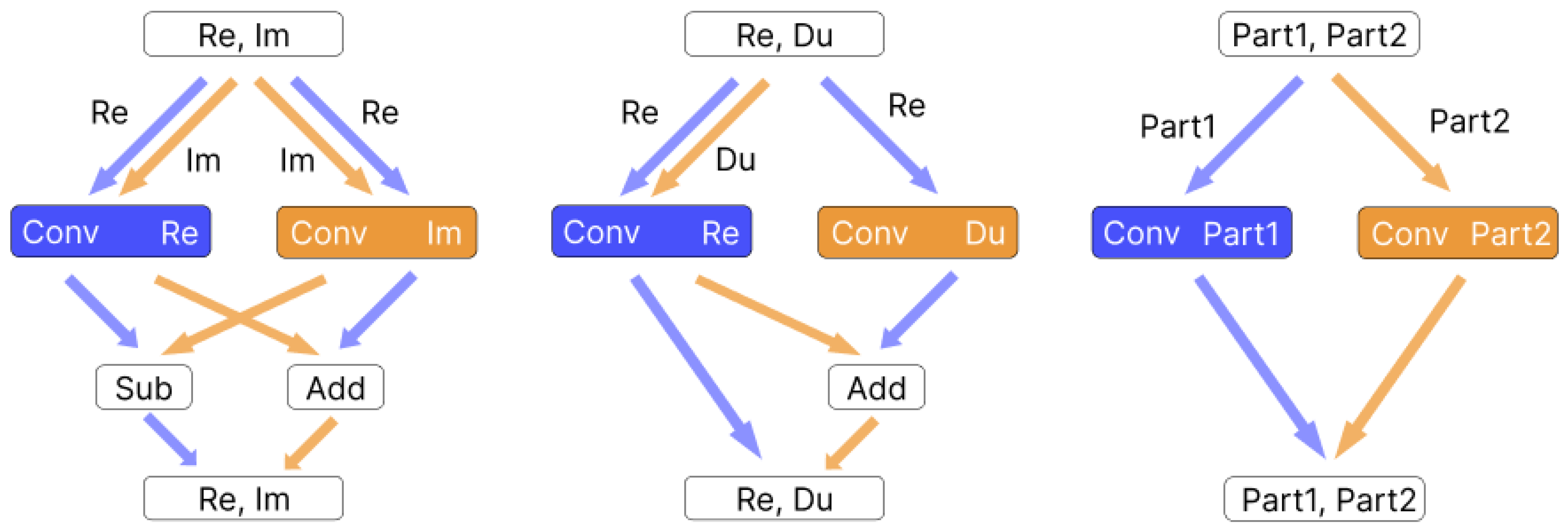
There is another reason for our interest in dual and double numbers. As real-valued layers expand to the hypercomplex algebras, the number of operations increases. The magnitude of this growth depends on the computational complexity of basic operations on the numbers. For example, one multiplication of two complex numbers is more expensive than four multiplications of real numbers. This influences the computational cost of the operators discussed in
Section 2. Thus, the convolution of a complex-valued input
with a complex-valued filter matrix
can be rewritten as
, which implies four real-valued matrix multiplications (see
Figure 1). The dual-valued convolution of a dual filter
and a dual input
evaluates
because
. This type of convolution only has three real-valued matrix multiplications (see
Figure 1), which gains a
theoretical performance speed-up, compared to the complex-valued convolution, and interconnects
x and
y in the process. As for double numbers, the cost of the naive implementation of the convolution is the same as for complex numbers because
. However, the features of double numbers enable variable substitution that allows changing to a so-called diagonal basis. Under that new setup, a double-valued convolution is effectively only two real-valued convolutions instead of four.
Section 3 of this paper is dedicated to the optimizations of hypercomplex networks, including the diagonal representation of double numbers (
Section 3.3). In this paper, we will mainly use the original representation of double numbers, for the sake of following the universal convention.
It is worth mentioning that double numbers in the diagonal representation have a significant flaw: the inability to connect
x and
y. However, the influence of this problem can be mitigated by a special batch normalization operator and/or an activation function for double numbers, which would make them connect. This adjustment is very important. As the experiments with real-valued networks have shown [
14], an appropriate batch normalization helps accelerate the training process and reach better accuracy. We will further discuss the components of hypercomplex-valued neural networks in detail.
In
Section 4 of this paper, we show that the adaptation of neural networks to the algebra of hypercomplex numbers allows us to improve precision. The important conclusion here is that the proposed types of neural networks, being barely explored so far, hold great potential for further research.
2. Methodology
This section is dedicated to the definitions of key elements of a hypercomplex neural network.
2.1. MindSpore Hypercomplex Data Representation
Until recently, only complex operators have been supported in popular frameworks, such as TensorFlow and PyTorch. The list of supported operations only contains basic manipulations with complex-valued tensors, as well as convolutional and linear layers. As of now, the situation has changed dramatically. MindSpore has become the first platform to support all the core layers needed to build second-order hypercomplex neural networks.
MindSpore allows researchers to create complex, dual, and double tensors, and perform all basic operations, such as slicing, concatenation, conjugation, and accessing both components of tensors. Convolution and linear layers are supported by MindSpore for all types of hypercomplex algebras of the second order. Other essential operators for deep learning, such as activation functions and algebra-specific batch normalization, are also integrated into MindSpore.
Within this framework, the hypercomplex tensor is represented as a two-channel real-valued tensor. Tensors of this shape are used as arguments and all operators return values in the same format. The peculiarities of every type of algebra are considered by a specific realization of network operators inside MindSpore, which interlinks the two channels of the tensors.
2.2. Hypercomplex Operators
The implementation of the operators mentioned above is based on our proposed method of generalizing the process of constructing building blocks for hypercomplex neural networks.
2.2.1. Convolution
Convolution is one of the most important operations in neural networks. In order to explain convolution in the hypercomplex algebra, we exploit the matrix representation of second-order hypercomplex numbers that use real numbers. The algebras of complex, dual, and double numbers
are all known to be isomorphic to the corresponding algebras of the second-order real matrices of the following form:
Recall that
. Therefore, the convolution of a hypercomplex filter
and a hypercomplex input
can be expressed as follows:
As mentioned earlier, we need to make three real-valued multiplications in the dual algebra (
,
, and
), but four in the cases of complex and double numbers (
,
,
, and
). For double numbers, however, changing variables, as shown in
Section 3.3, enables moving to the diagonal representation, where the algebra becomes isomorphic to the algebra of real matrices of the following form:
, and the convolution only requires two convolutions in real numbers.
2.2.2. Linear Layer
Linear (fully connected, dense) layers are commonly used in neural networks as the head blocks in the CV (computer vision) domain and as the main operators in NLP (natural language processing) models. To generalize linear layers for the two-dimensional algebras, we use the matrix representation of second-order hypercomplex numbers. In the end, a linear layer with hypercomplex inputs and weights is equivalent to the superposition of real-valued linear layers:
where
stands for a real-valued linear layer, with
w,
b, and
x denoting weights, bias, and the input, respectively.
2.2.3. Average Pooling
The average pooling operation implies calculating the arithmetic mean for each patch of the feature map. This means collapsing every
square of the feature map into its average value. This is equivalent to convolution, with the stride being equal to the kernel size, where kernel weights are real numbers that are equal to
. Because the kernel
in this particular case is purely real,
, and the convolution formula can be simplified as follows:
From this expression, average pooling is equivalent to two real-valued average pooling operations, with each independently applied to every component of the input data
:
2.2.4. ReLU
Activation functions are used to introduce non-linearity into neural networks. There are multiple activation functions based on real numbers, and greater varieties are based on hypercomplex numbers. Among the real-valued activations, there is a family of
-type functions, which do not suffer from the vanishing gradient problem. This property makes them quite stable. Functions of this type are used in the complex algebra as well. For example, the authors of [
15] applied
to the real and imaginary parts separately. In this paper, we extend this definition and apply it to other algebras:
This activation approach is not perfect. First, in contrast to
on real numbers,
may not be equal to 0 or
u. Second, the real and imaginary parts are processed independently and, therefore, are not fully interlinked. Despite that, the method shows good experimental results, and its obvious advantage is simplicity.
2.3. Norm of Hypercomplex Numbers
In deep learning, the ability to properly update model parameters is important for training a model with better accuracy on a test dataset. The weights may not be efficiently updated if elements of intermediate tensors are not normalized due to the gradient explosion or vanishing problem. In real-valued models, the solution is the batch normalization procedure. The idea is to balance tensor elements based on the variance of the batch. To develop a counterpart operator for neural networks based on second-order algebras, we must find an equivalent of the absolute value function. Here, we define a concept of the norm (or modulus) of hypercomplex numbers. In mathematical or physical literature, the modulus of a complex number is traditionally defined as
However, the generalization of this method to other types of hypercomplex numbers does not work quite well:
This result is hardly applicable to our purpose. The dual norm does not depend on the dual part. In the case of double numbers, the function is not well-defined for half of the elements. In [
16], the authors derive the norms of dual numbers that are free from the mentioned downsides. Here, we extend the idea to develop the formula for all hypercomplex numbers of the second order, and make sure that it replicates the expression of the standard norm of complex numbers (
1). The approach is based on the matrix representation
of a hypercomplex number
. We derive the norm of this matrix and associate it with the norm of a hypercomplex number. For the matrix norm, we use the following definition:
After some straightforward mathematical manipulations (see
Appendix A), we obtain the following formula for the hypercomplex number norm:
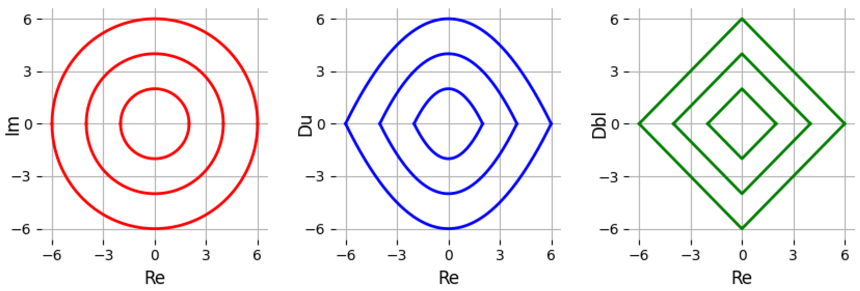
To show the differences among the proposed norms for the hypercomplex algebras, we depict
equal to 2, 4, or 6 with contour lines in
Figure 2. It is shown that the contour lines of dual and double norms are closer to the center than the corresponding contour lines for complex numbers. Different norm expressions have different effects on batch normalization for the dual, complex, and double algebras.
2.4. Batch Normalization
As mentioned in the previous section, batch normalization is very important for a successful training process and convergence to high-metric values. In its original form [
14], it can only be applied to the real-valued models. This approach includes the normalization of each dimension of the
k-dimensional input:
After this transformation, the mean of
is equal to zero, and the standard variance is equal to one. However, it is better to make the mean and variance trainable parameters. In practice, it is achieved by performing additional scaling and shifting:
The technique of batch normalization has been extended to complex inputs [
15]. The authors suggested transforming the inputs using a covariance matrix so that the real and imaginary parts do not correlate. However, we cannot generalize this method explicitly; this is because—for dual numbers—the pseudo-covariance
C cannot be equal to zero:
with at least the real parts always being greater than zero. Therefore, we need to find an alternative way to generalize batch normalization to all types of hypercomplex algebras of the second order. In this paper, we present a method based on the norm concept of hypercomplex numbers, as derived in the previous section, and compare the proposed method for complex numbers with the idea presented in [
15].
First, we define the mean value in the traditional channel-wise way, which is the same for all algebras:
Then we define the variance that is specific to the type of hypercomplex algebra:
where
is determined by (2). Then we transform the input as follows:
where
is a small number needed to avoid division by zero. The last step is hypercomplex channel-wise scaling and shifting:
where
and
are the hypercomplex weights and bias, accordingly.
In the specific case of complex numbers:
So, dividing the centered input by
provides the covariance
. Note that, in general, pseudo-covariance is not equal to zero:
Since
and
may correlate,
. Despite that, as shown in
Section 4, using this method results in good metric values. We emphasize that MindSpore is the only framework that has implemented this mathematically justified batch normalization technique.
We conduct an ablation study of the proposed batch normalization technique. For this purpose, we construct a hypercomplex LeNet-5 model and vary the normalization. The following approaches are considered: real-valued channel-wise normalization, covariance-based normalization from [
15], and algebra-aware normalization (
3) based on the proposed hypercomplex norm (
2).
We show that all normalization types lead to about the same results on the MNIST dataset after 20 epochs (see
Table 1). Nevertheless, the proposed hypercomplex normalization is more beneficial because it can be further fused with a previous convolutional layer (
Section 3.4).
2.5. Backward Propagation of Loss Function Gradient
An important part of neural network training is gradient calculation. Computing the loss function gradient relies on the backpropagation algorithm, which exploits the chain rule. In this paper, we explore the gradient propagation problem in the algebra of hypercomplex numbers. The classic definition of the derivative of a function
of a hypercomplex argument
, where
v and
w are real-valued functions, is
This limit can only exist if it is well-defined when
approaches zero along the real axis (
) or the imaginary axis (
). In either case, it should provide the same result. Equating these special cases, we obtain the general equivalents of Cauchy–Riemann equations:
Functions that satisfy these equations are called holomorphic. In practice, this is a strong restriction, and most of the existing operators do not satisfy the Cauchy–Riemann criteria. To overcome this, we use the approach invented by Wirtinger for complex numbers [
17]. It applies variable substitution in order to rewrite a complex-variable function
as a holomorphic function of two arguments
. This idea was applied in [
18] to derive the gradient of double numbers. Here, we extend this approach to all second-order algebras:
For complex and double numbers, we can easily eliminate by multiplying both the numerator and denominator by and we end up with in the denominator. However, we cannot perform the same trick for dual numbers because—in that case— is equal to zero. Thereby, we must keep in the denominator. We must also keep the expressions with in the numerator, because they will contribute to the component with if they cancel one of the with .
Here, we clarify what exactly must be calculated in order to update hypercomplex weights. With complex-valued networks, researchers usually treat the real
and imaginary
parts of weights
as separate real-valued channels and update them using the real-valued derivative of a loss function:
We generalize these calculations for all hypercomplex numbers of the second order, considering:
We define the expression inside the parenthesis as a hypercomplex gradient and calculate it via the gradient of a hypercomplex operator
f (see
Appendix B) as follows:
It is noteworthy that
can be expressed in terms of
u and
, i.e.:
With dual numbers, we keep the part with , despite the fact that it must be equal to zero, as stated above.
We implemented this formula for dual algebra. This method yields results consistent with the calculations from two real-valued derivatives. Our experiments show that the training time is approximately the same as well. However, the performance can be improved if operations on hypercomplex numbers are implemented as instructions on the hardware level.
3. Optimizations
In this section, we discuss technical methods to speed up the execution of testing and/or training models based on hypercomplex numbers. While this is an important engineering challenge, it is not as crucial as achieving the best possible accuracy. We focus on searching for equivalent transformations that speed up hypercomplex operators and do not affect the network output or metric values. These methods are not universal, so the final acceleration depends on the model architecture.
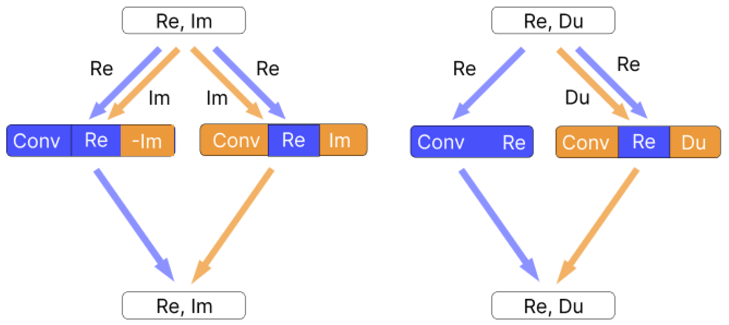
3.1. Hypercomplex Convolution Grouping
We express a hypercomplex convolution through a certain number of real-valued convolutions (
Section 2.2). For complex- and dual-valued convolutions, we have to conduct extra addition and/or subtraction (see
Figure 1). It is possible to “insert” these arithmetic operations into the real-valued convolutions. In order to do that, we concatenate the components of the input and perform a similar operation for the weights (see
Figure 3). This approach increases memory usage and necessitates tensor duplication, using the best-optimized solution. Note that, in the case of the complex-valued convolution, we need to invert the imaginary part of the weights when we calculate the real part of the output. Thus, we implement subtraction. Although the negation operation must be cheap in terms of execution time, it is possible, if needed, to store the inverted weights in advance to speed up the inference at the cost of a larger model size.
3.2. Karatsuba’s Algorithm
Karatsuba’s algorithm is a well-known technique used for the optimization of complex number multiplication. It can also be applied to convolutions and linear complex-valued operators. For example, a linear operator can be rewritten as three real-valued linear operators:
where
,
, and
. Fewer matrix multiplications come at the expense of a greater number of additions and subtractions. Therefore, Karatsuba’s algorithm performs better for convolutions with large batch sizes and weight widths, where multiplications are more expensive.
3.3. Diagonal Representation of Double Numbers
In
Section 1, we briefly mentioned the representation of double numbers in the diagonal basis. Here is its mathematical definition:
The computation complexity of multiplication is halved in this form:
Section 2.2 shows the isomorphism between hypercomplex numbers and matrices of the second order. Then, a convolution of double numbers in the diagonal form can be expressed as follows:
which implies the convolution calculation as two component-wise real-valued convolutions
and
. Thus, we define new variables as
and
, so that
. Batch normalization can be updated accordingly. Moving from the regular representation to the diagonal one is identical to the affine transformation of the plane of double numbers. The norm of a double number
is expressed as
.
As discussed before, the downside of using the diagonal representation is that
x and
y are poorly interlinked and are almost equivalent to two independent real numbers. The batch normalization based on the norm of double numbers partially solves this issue. Average pooling and linear functions are calculated for both components independently, because they are special cases of convolution. The relationship between two components is introduced through non-linear activation functions. The ReLU implementation
works well with the classic representation of double numbers. It makes sense to reuse this by transforming the intermediate tensor to the classic representation before applying the component-wise activation. In the end, the formula looks as follows:
This activation function requires more operations compared to the base ReLU implementation. However, in combination with the enhanced performance of the convolution, it allows the model to save precision with significant acceleration.
3.4. Equivalent Transformations
Real-valued convolutional neural networks can be accelerated by means of a fusing convolution with a subsequent batch normalization layer into a convolution with new parameters, as described by the following equations:
where
and
are weights and biases of the fused convolution,
W and
b are weights and biases of the original convolution,
,
,
,
are the mean value, variance, scale, and shift of the batch normalization layer, respectively. The × operator is an element-wise multiplication.
This transformation leads to improved inference time and memory conservation. In the case of real models, some frameworks have already implemented this optimization. For example, the ONNX simplifier does that automatically for models in the ONNX graph format.
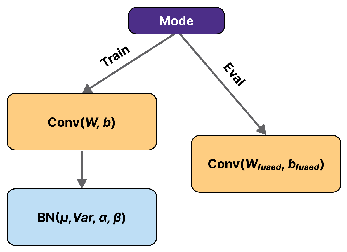
Hypercomplex operators require more resources, which makes this optimization even more critical. However, so far, there is no automated tool that could apply it to hypercomplex models. For example, an attempt to export a model to ONNX and use the ONNX simplifier would fail. Currently, the ONNX simplifier cannot fuse a sequence consisting of hypercomplex convolutional and batch normalization layers. So, we introduce a new layer called CBN (Conv+BN), which behaves differently depending on the mode. During training, it behaves as the original sequence of two layers, and in the evaluation mode, it works as a convolution with fused parameters (
Figure 4). These parameters are pre-calculated according to Formulas (
4) and (
5), assuming that all multiplications follow the rules of arithmetic of hypercomplex numbers.
Our CBN layer is implemented in MindSpore to improve the inference times of hypercomplex models.
4. Results
To explore the generalization of neural networks on hypercomplex numbers, we develop a demonstrative network to predict values of noised hypercomplex functions. In addition, we conduct a series of experiments with hypercomplex models for computer vision and signal processing tasks. We compare the results of these networks with the results of real-valued models of the same architecture.
4.1. Hypercomplex Toy Net
We start with a demonstrative neural network designed for predicting the values of noisy functions of a hypercomplex argument. Our toy network consists of two linear layers and a sigmoid-type activation function (see
Appendix C) in between. This architecture remains the same for all the algebras, but for every algebra, we use its implementation of the operators.
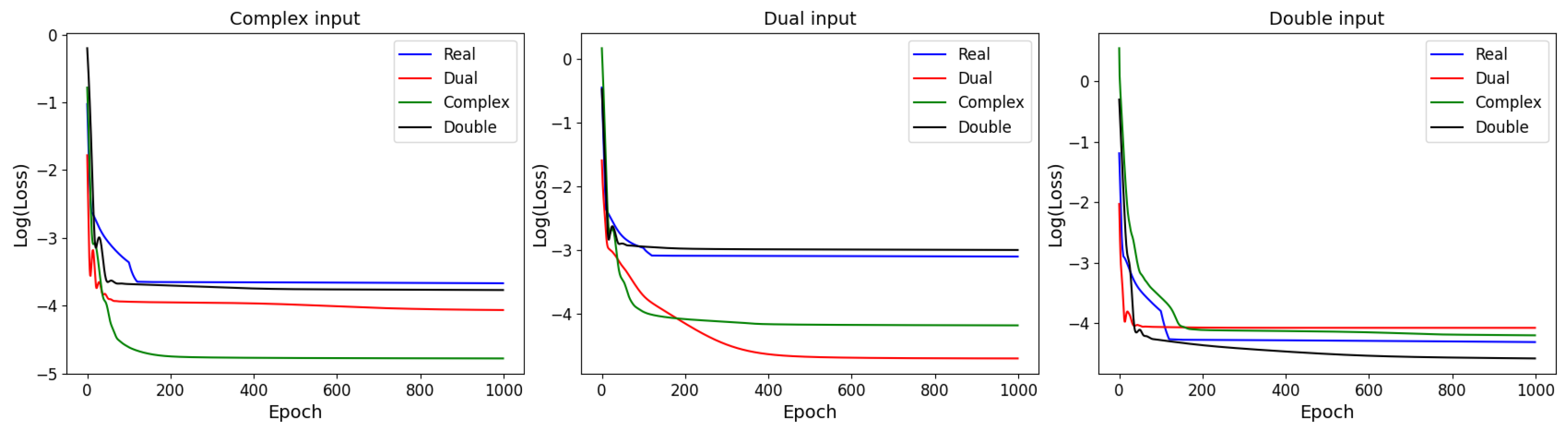
In order to show the advantage of hypercomplex models, we compare their results with the result of a real-valued model of the same architecture. The mean square error (MSE) is used as a loss function. We train these four models for 1000 epochs with the same number of parameters to predict values of two functions:
—the Airy function of the first kind and
—the Bessel function of the first kind of the third order. We also add noise with a normal distribution to the values of functions in a training set (and a testing set). The results are shown in
Table 2.
It is clear from
Figure 5 and
Table 2 that the lowest mean square error is achieved by a neural network belonging to the same type of hypercomplex number as the function argument. For example, a complex-valued function is best predicted by a complex-valued model, and so on. Thus, we conclude that networks based on hypercomplex numbers can learn dependencies or patterns that lie in the corresponding algebra.
4.2. Classical CV Problems
Before we move on to solving CV classification problems, it is necessary to clarify the process of data preparation. To convert a real-valued image to the hypercomplex format in this research, we use a more general method compared to the one proposed in [
5]. In [
5], the authors convert a real-valued image to a complex form by
, claiming that this type of encoding captures the channel correlations and hue shift. In this paper, we generalize this idea and use the following transformation
, which we call the color combination. However, there is another possibility to generate an imaginary component by processing the real input data using several layers [
15].
We take ResNet18 architecture [
19] as the basis of our model that is generalized to hypercomplex algebras of the second order by replacing real-valued operators with their counterparts in hypercomplex algebras. We use stochastic gradient descent with 0.9 momentum to optimize real-valued loss functions by treating the real and hypercomplex parts as separate real-valued channels. To transform hypercomplex features into the real ones, we concatenate both components of the output into a double-sized real-valued tensor before feeding it to the terminating fully connected layer. The cross-entropy loss between the input and the target is used as a criterion for these problems. The total number of epochs is 200 for every experiment. The learning rate is scheduled by the cosine annealing rule, starting from
. The size of a mini-batch is 8. Every model is trained 5 times with different seed numbers, and the median value of the accuracy is taken to negate the effects of fluctuation. Our image classification results on CIFAR-10, CIFAR-100, and SVHN are presented in
Table 3.
One can observe in
Table 3 that all models based on the second-order numbers achieve higher accuracy compared to the real one. In addition, the complex-valued neural network shows better metric values compared to other hypercomplex models.
Table 4 demonstrates how remarkably inference time is reduced by using the CBN equivalent transformation described in
Section 3.4. The effect is so dramatic that, from now on, it is worth considering models with CBN only. Figures from the CBN column of
Table 4 are used as the baseline for the assessment of other optimizations, which are discussed below. These figures also indicate that transferring from a real model to a hypercomplex one significantly increases computational complexity.
Table 5 shows the effect of optimization on the second-order hypercomplex models.
The worst performance is shown by the naive double-valued network, but the transition to the diagonal representation accelerates it dramatically. Still, the double-valued network is not an optimal model because it shows the worst accuracy among all hypercomplex models (see
Table 3). As for the complex- and dual-valued networks, grouping convolutions helps to improve the inference time, and for the complex-valued network, the implementation of Karatsuba’s algorithm helps even more.
Our main idea is that dual-valued neural networks, as well as complex-valued ones, allow different channels to interact with each other due to the internal connection between real and dual parts. This inner complexity should be exploited; possibly, more sophisticated input preprocessing can lead to even better accuracy for these more complicated networks.
4.3. Gravitational Waves Detection
This part is dedicated to the solution of a signal detection task using hypercomplex networks for the G2Net dataset. This dataset consists of simulated noised signals that are similar to gravitational waves recorded by a system of three ground-based laser interferometers: LIGO Hanford, LIGO Livingston, and Virgo [
20,
21,
22]. Generally, gravitational waves are emitted during cosmic events, such as the merging of black holes [
20]. The G2Net dataset contains records of emulated events of the same nature.
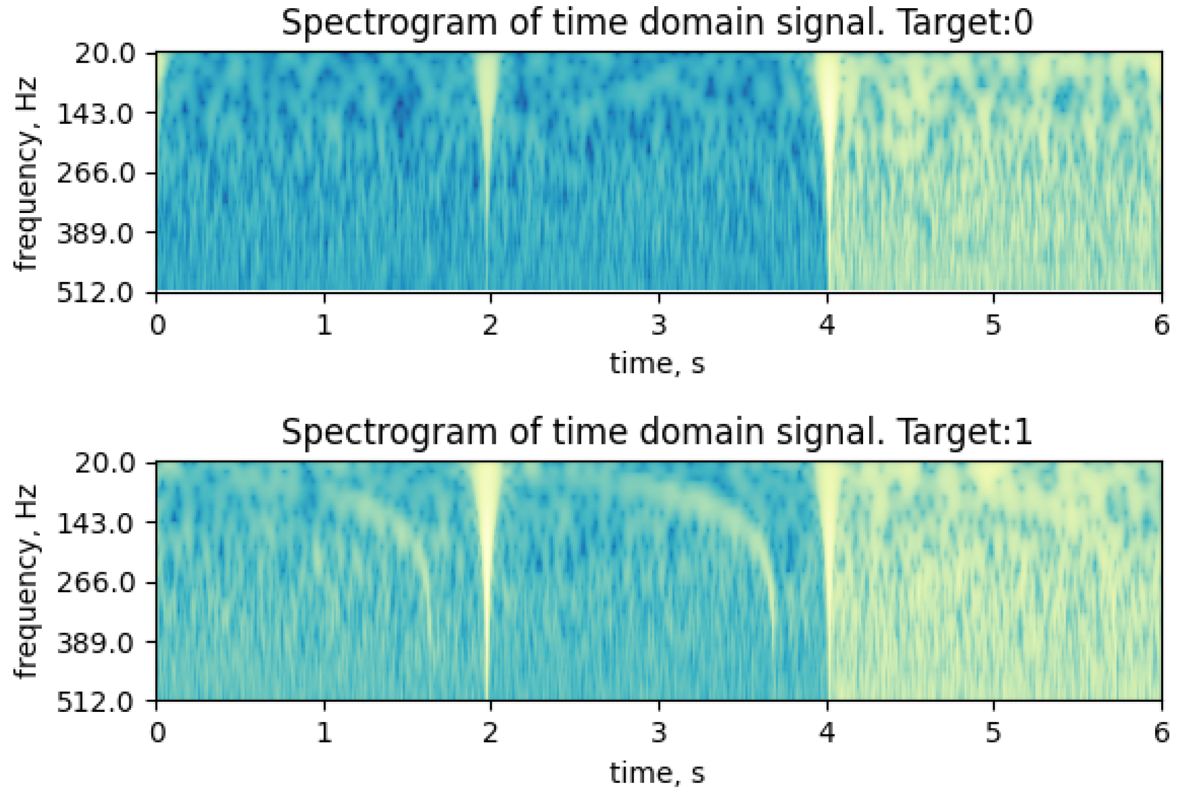
To classify the original signal, we preprocess data to an image and run it through our neural networks. The aim of preprocessing is to build a representative frequency map of the original signal. The CQT algorithm [
23] is considered efficient for analyzing gravitational waves.
This preprocessing transfers the time series into the frequency portrait (see
Figure 6), which is treated as an image in further steps. Thus, the variations of frequency characteristics of the signal at certain moments are reflected as visual features, such as specific shapes and colors, in the resulting image. To classify the image obtained after CQT, we again use the ResNet18 model, whose operators are changed to the corresponding ones in ad hoc algebras.
The model is optimized using the stochastic gradient descent algorithm with a momentum of 0.9 and weight decay of for regularization. The regularization is enhanced by adding dropout with a value of 0.2. The scheduler for the learning rate uses the cosine annealing policy with , and the initial value of lr is set to . Training lasts 30 epochs.
From
Table 6, one can see that all models on the hypercomplex algebra outclass the real-valued model in both accuracy and AUC ROC (area under the receiver operating characteristic curve) metrics. The best result is achieved by a dual-valued neural network.
4.4. Music Transcription Task
In this section, we present the results of training hypercomplex networks on an automatic music transcription task. The experiments are performed on the MusicNet dataset [
24]. In order to convert the input signal into a complex-valued tensor, we use the Fourier transformation. We reuse the DeepConvNet architecture developed in [
15], with its building blocks replaced with the corresponding layers designed for specific algebras.
Table 7 shows that hypercomplex networks significantly outclass the same model on real numbers. The best figures are shown by a dual-valued network.
Next, we present the results of inference time measurement on GPU (see
Table 8). The first column presents the measured inference time of the baseline model, and the second one shows the inference time of the same models after optimizations.
The optimizations of the complex-valued network include convolution grouping and Karatsuba’s algorithm for the most expensive linear operator. For dual numbers, we only use convolution grouping, which provides a small performance gain. The double-valued operators are redesigned to take advantage of the diagonal representation. In all cases, batch normalization operators are fused with the preceding convolutions. The experiments are performed with a batch size of 8. The dual-valued model outperforms all other second-order hypercomplex models. The double-valued network, despite its diagonal representation, yields the poorest results due to the significant overhead associated with activation functions.
5. Discussion
5.1. Summary
Improving model accuracy is the cornerstone of many modern research studies in the field of deep learning. This target can be achieved by different methodologies, such as dataset expansion, changing the training procedure, variation of neural network architecture, and so on. In this study, we offer a take-and-go recipe on how to enhance the model’s generalization ability. Namely, one needs to replace real-valued layers with the corresponding complex, dual, or double counterparts, without any modifications to the overall architecture. Generally speaking, it is impossible to predict which kind of algebra will be better for a particular task. To overcome this obstacle, we define a universal approach to developing operators based on any kind of hypercomplex algebra of the second order. This allows researchers to design an architecture of neural networks without heavy dependence on a specific kind of algebra.
In our experiments on the CV, G2Net, and MusicNet tasks, complex and dual-valued models have shown the best results. Nevertheless, neural network construction is a multi-criteria problem. If inference and training times are important, then dual-valued models are often preferable, whereas the complex-valued ones can provide extra accuracy when the timing is not so critical.
5.2. Limitations and Outlook
A limitation of the present study is our sole method of converting real-valued data to hypercomplex numbers for CV problems. It is possible that suboptimal data preprocessing resulted in small gains on these tasks. We plan to explore new methods of real input transformation.
Another unsolved issue is how to identify the type of algebra—for a particular task—that would have the best performance among the hypercomplex algebras of the second order. We will be looking for some heuristic methods that predict the best algebra without training the models with all types of algebras.
In conclusion, the presented methodology exhibits significant promise in enhancing the efficiency of transformer-based architectures. Also, we plan to develop a hypercomplex network compression methodology because we did not find any compression algorithms for non-real models.

 ,
, 


