Equilibrium Analysis for Batch Service Queueing Systems with Strategic Choice of Batch Size

Abstract

Various transportation services exist, such as ride-sharing or shared taxis, in which customers receive services in a batch of flexible sizes and share fees. In this study, we conducted an equilibrium analysis of a variable batch service model in which customers who observe no waiting customers in an incomplete batch can strategically select a batch size to maximize the individual utilities. We formulated this model as a three-dimensional Markov chain and created a book-type transition diagram. To consider the joining/balking dilemma of customers for this model, we proposed an effective algorithm to construct a necessary and sufficient size of state space for the Markov chain provided that all customers adopt the threshold-type equilibrium strategy. Moreover, we proved that the best batch size is a non-decreasing function for i if the reward for the completion of batch service with size l is an increasing function of l assuming that a tagged customer observes i complete batches in the system upon arrival; in other words, the fee decreases as the batch becomes larger. We then derive several performance measures, such as throughput, social welfare, and monopolist’s revenue. Throughout the numerical experiment, a comparison between the present variable batch service model and regular batch service model in which customers were served in a constant batch, was discussed. It was demonstrated that the three performance measures can be optimized simultaneously in the variable batch service model, as long as the fee was set relatively high.

1. Introduction

Batch service queueing systems have frequently appeared in recent transportation services. Examples are shared taxis or ride-sharing services, such as Uber or Lyft. In these systems, customers typically form a group, ride in the same vehicle, and share a move. Then, the concern over the ‘best’ batch size has risen. Customers generally share fees with other customers in a batch; therefore, the financial burden on a customer decreases as the batch size increases. However, customers must experience longer waiting times to create a larger batch, that is, to wait for the arrival of other customers. Therefore, to determine the ideal batch size, constructing a model that considers both financial and time costs is necessary.

In the field of queueing theory, many studies that consider the behavior of strategic customers have been conducted to discuss systems from an economic viewpoint. Regarding batch service queueing systems, some studies have been conducted on models in which strategic customers are served in a batch with a constant batch size. However, to the best of our knowledge, a model in which customers strategically select a batch size to maximize their individual utility based on the state of the system has never been studied. In this study, we analyzed such a dynamic batch service queueing system with strategic customers (see the detailed explanation in Section 2). From a managerial perspective, for modern transportation systems, a scope for discussion regarding the effect of the strategic choice of batch size on both social welfare and administrator revenue still exists. In addition, the analysis of this model is challenging from a modeling perspective. The arrival interval of complete batches to the system depends on the congestion level in the present model, whereas the arrival process in the constant batch size model can be expressed by the Erlang distribution with a rate equivalent to the arrival rate of customers and shape, which is determined by the batch size.

The batch service queueing model was pioneered by Bailey [1], and many studies have been conducted for more than half a century. We refer to the thorough survey in [2] and only cite the research that handles a non-constant batch size:

• General bulk-service (GBS) queues. The GBS rule (or $(a,b)$-rule) is explained as follows. The server will start to provide service only when at least ‘a’ customers are in the queue, and the maximum service capacity is ‘b’. This type of queue has been studied extensively (see, e.g., [3,4,5,6,7,8,9,10,11,12,13]). As finite buffer models, a few studies have been conducted (see, e.g., [14,15,16,17,18,19]). In addition, the models of batch-size-dependent service have been studied [13,18].
• Batch service queue with a random batch size. The models where the size of a batch service follows an arbitrary distribution have been conducted [20,21]. In addition, the model of batch-size-dependent service has been studied [22].

Queues with strategic customers were first investigated by Naor [23], who studied the joining/balking dilemma in an observable M/M/1 queue. Many studies have been conducted on the game-theoretical analysis of queues (see surveys [24,25]). Previous studies on batch service queueing systems can be summarized as follows:

• Regular batch service. Several studies have considered the system in which the service is conducted by a batch of constant batch size. The observable and unobservable models [26] as well as the partially observable models [27,28] have been studied. A simple extension to the multiple server model of the observable case has also been conducted [29]. Furthermore, an equilibrium analysis of a batch service queueing system considering the limitation for the number of service facilities (e.g., cars in the application of real life) has been studied [30].
• Clearing system. Some research has been conducted on the clearing system in which the service facilities periodically remove all present customers. The clearing system with strategic customers was first studied in [31], which assumes an alternative environment scheme. Moreover, a clearing system with bounded rationality was considered [32]. Furthermore, many policies of information disclosure levels were compared (see, e.g., [33,34,35]). The analysis of a transportation system with constant intervisit time and heterogeneous customers was also conducted [36].
• Choice among multiple capacity services. Several studies have been conducted on the strategic choice among infinite server systems with regular batches and single-server systems of single service [37,38,39,40,41]. These studies showed interesting Downs–Thompson and Braess-type paradoxes through the equilibrium analyses of this type of model. Some recent studies considered the routing problems in a parallel clearing system [42] and the strategical choice between a single service and batch service with size two on the basis of waiting time cost [43].

This study is related to pricing control among different types of services. The aforementioned study on clearing systems [34] also considered the pricing scheme. Additionally, we cite the following papers:

• Priority queues. One fundamental method of pricing control is the introduction of priorities. In priority queues, customers can buy the priorities with the additional fee and replace the ordinary (not buying priority) customers, saving the waiting time (see, e.g., Chapter 4 in [24] and [44,45]). Both social optimization and revenue maximization were considered in [44].

In this study, we proposed a new type of observable batch service queueing system. This mechanism can be briefly explained as follows: If no complete batch exists when a new customer arrives in the system, he can decide the size of his batch to be served (or balking the system) based on the expected utility, which depends on the expected sojourn time and fee. A new customer, who finds any waiting customers in an incomplete batch, decides to join the batch or balk the system based on expected utility. This model corresponds to the recent shared-taxi or ride-sharing system, where customers create a group of favorable size based on the shared fee and the expected time cost, which is influenced by the arrival rate of customers and the congestion state of the road.

From a technical perspective, we extended the two-dimensional Markov chain in the regular batch service model [26] to a three-dimensional Markov chain that considers the batch size of an incomplete batch. We found that our Markov chain forms the ‘book-type’ state space. By leveraging this form, we calculated the expected sojourn time for a tagged customer. To consider the joining/balking dilemma of customers for this model, we proposed an effective algorithm to construct a necessary and sufficient size of state space for the Markov chain provided that all customers adopt the threshold-type equilibrium strategy. Furthermore, we proved that the best batch size (for the first-arriving customer who observes zero waiting customers in an incomplete batch), provided that a tagged customer observes i complete batches in the system upon arrival, is a non-decreasing function for i if the reward for the completion of a batch service with size l is an increasing function of l; in other words, the fee decreases as the batch becomes larger.

We conducted various numerical experiments on throughput, social welfare, and revenue. In the experiment, we introduced the notions of ‘fixed fee’ and ‘sharing fee’. A fixed fee refers to the fee that all customers pay to receive the service, regardless of their batch size. The sharing fee refers to the fee for a batch, that is, the fee for a person is the sharing fee divided by the batch size. In this setting, we observed customer behavior by considering the trade-off between time and money.

The proposed model encompasses Naor’s model [23] and the observable regular batch service model [26]. Throughout the numerical experiment, we demonstrated some performance measures: throughput, social welfare, monopolist’s revenue, and expected sojourn time in the variable batch service model show more stable performance than the regular batch service model if both sharing and fixed fees are set to some extent.

In summary, the important messages of this study from the application point of view are as follows: the system where the administrator enables customers to form the favorable size of the batch to maximize their utility is meaningful, particularly when the fixed and sharing fees are relatively high. The proposed model does not show extremely bad results for any arrival rate as long as both fees are set in a well-balanced manner compared to the regular batch size model. This indicates that the proposed model is a robust model for the fluctuation of customer demand. In addition, the introduction of the variable batch service model can lead to optimizing all of the throughput, social welfare, and monopolist’s revenue, simultaneously, compared to the regular batch service model under a high setting of the fees. On the other hand, the variable batch service model shows bad performance when the fees are set low.

The remainder of this paper is organized as follows. The settings of the model are described in detail in Section 2. Section 3 presents the analysis of the model. We present several numerical examples in Section 4. Finally, Section 5 concludes the paper.

2. Modeling

This section describes the model settings in detail. Customers arrive at the queue according to a Poisson process at a rate $\lambda$ one-by-one and receive the service as a batch. The (single) server service time for a batch follows an exponential distribution of the parameter $\mu$ regardless of the batch size. The reward for receiving a service is defined by R and the customer fee for a service with batch size l is denoted by $p_l$. Therefore, the reward for receiving a service in a batch of size l can be regarded as $R_l=R-p_l$. Furthermore, $R_l$ becomes a function of l with upper bound R. We assume that all customers are rational and have a common knowledge of the aforementioned information. Moreover, we assume that the system is observable; that is, customers can observe the number of complete batches in the system, the number of waiting customers in an incomplete batch, and the size of the incomplete batch (when it will become full) at the time of their arrival.

If a customer finds no waiting customers in the incomplete batch (i.e., all batches in the system are complete batches and he cannot join them) and i complete batches in the system, he decides to adopt the best batch size $l^{*}$ according to the following definition:

$$l^{*}=\left\{\begin{array}{cc}0,\hfill & \mathrm{if}{R}_l-C{W}_{i,0,l}<0\mathrm{for}\forall l,\hfill \\ \max \mathbb{D},\hfill & \mathrm{otherwise},\hfill \end{array}\right.$$

(1)

and

$$\mathbb{D}=\underset{l\in \mathbb{N}}{arg}\max (R_l-C{W}_{i,0,l}),$$

where $W_{i,0,l}$ denotes the expected sojourn time for a tagged customer who observes zero waiting customers in an incomplete batch, under the condition that the number of complete batches is i at the arrival time point, and the customer adopts batch size l. Here, note that $\max \mathbb{D}$ stands for the maximum element (batch size) in set $\mathbb{D}$. If no incentive exists to join the system for any batch size, we let $l^{*}$ be 0.

If a tagged customer finds i complete batches, $k(>0)$ customer(s) in the incomplete batch, and the batch size that he receives from the service is l at his arrival time point, they join the system with probability $q_{i,k,c}$ as follows:

$$q_{i,k,l}=\left\{\begin{array}{cc}1,\hfill & \mathrm{if}{R}_l-C{W}_{i,k,l}\ge 0,\hfill \\ 0,\hfill & \mathrm{if}{R}_l-C{W}_{i,k,l}<0,\hfill \end{array}\right.$$

(2)

where $W_{i,k,l}$ represents the expected sojourn time (if he joins) under the condition that the number of complete batches and the number of customers in the incomplete batch are i and k, respectively, at his arrival time point with batch size of l.

We assume that not all customers are allowed to change their decisions (best batch size, join/balk) after deciding. For simplicity, we assume that customers are in favor of joining a larger batch; that is, when they are indifferent between joining and balking, they choose to join, and when they are indifferent among multiple batch sizes, they choose the largest batch, similar to that in [26].

Let $I\left(t\right)$, $K\left(t\right)$, and $L\left(t\right)$ denote the number of complete batches, number of waiting customers in the incomplete batch, and the size of the incomplete batch when it becomes full, respectively, at time t. Then, $\left\{\right(I\left(t\right),K\left(t\right),L\left(t\right));t\ge 0\}$ becomes an irreducible three-dimensional Markov chain with state space $\mathcal{U}$, where

$$\mathcal{U}=\mathbb{Z}\times \mathcal{V},$$

$${\mathcal{V}}_1=\left\{(0,1)\right\},$$

$${\mathcal{V}}_a=\{(1,a),(2,a),\dots (a-1,a)\},a\geqq 2,$$

$$\mathcal{V}=\{{\mathcal{V}}_1,{\mathcal{V}}_2,{\mathcal{V}}_3.\dots \}.$$

Notably, $L\left(t\right)=1$ is a special case because $L\left(t\right)$ accepts 1 automatically whenever $K\left(t\right)=0$ holds, because of the aforementioned definition. Here, we let $I,K$, L denote the random variables in the steady state, that is, the variables under $t\to \infty$.

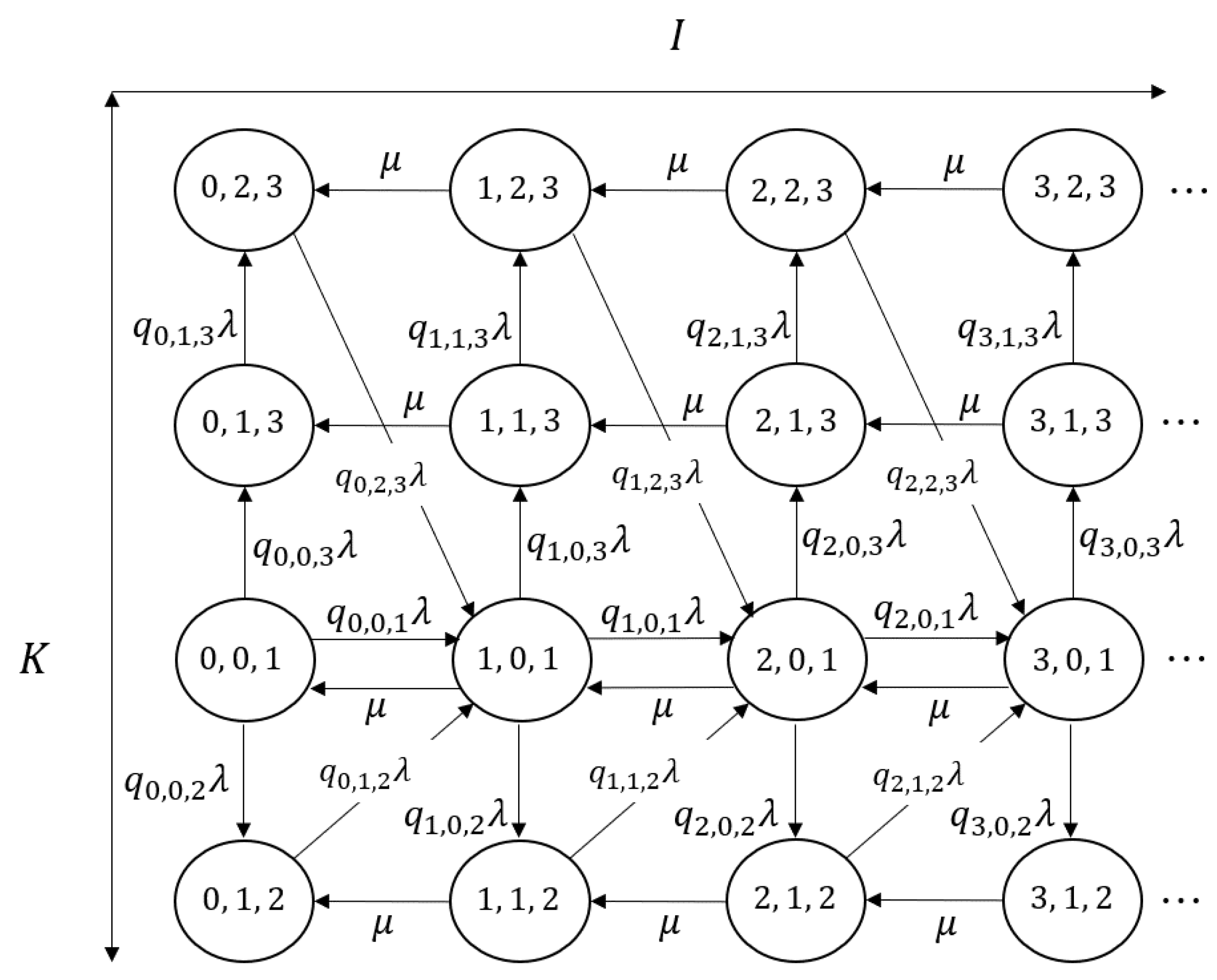
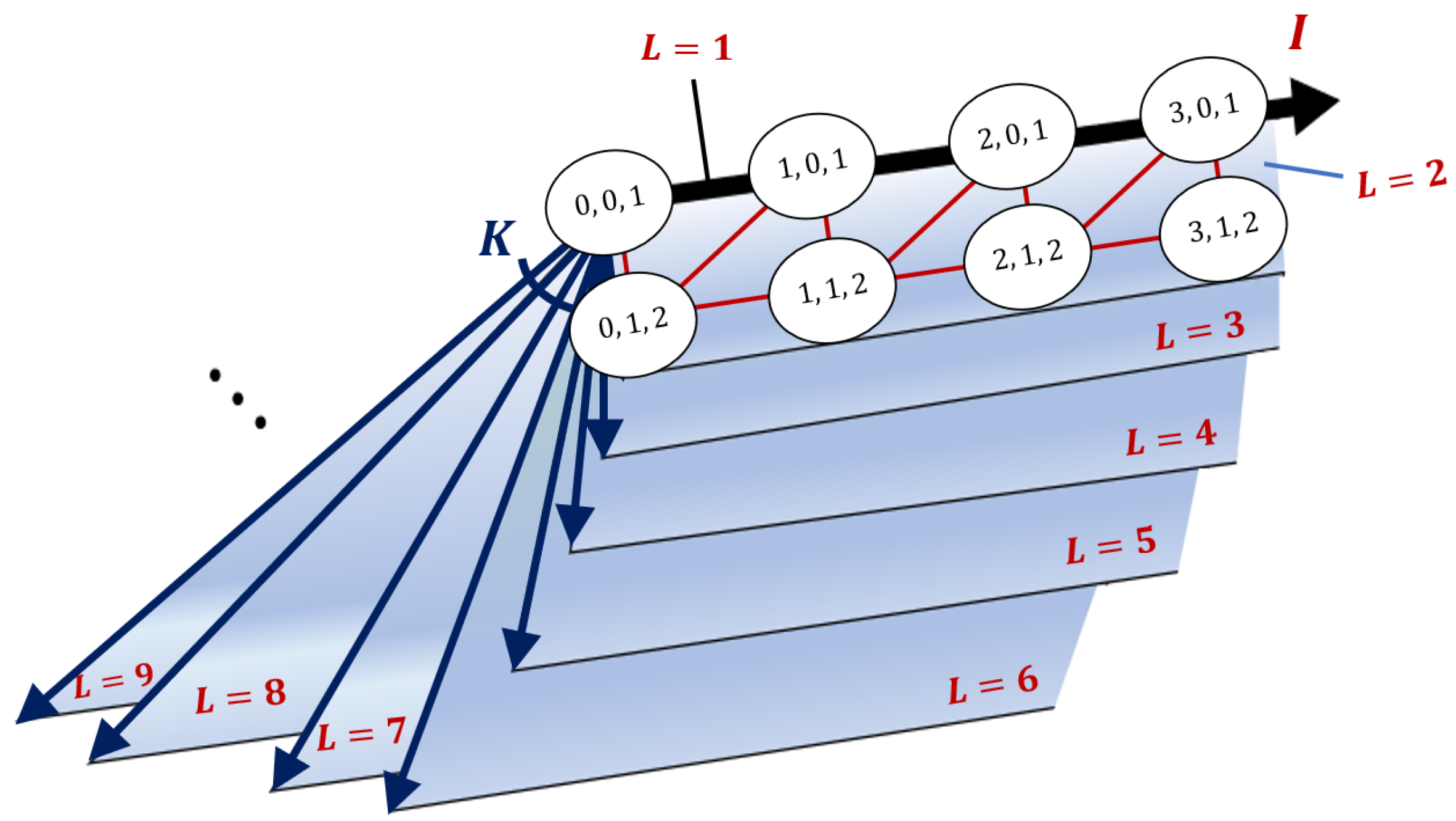
We refer to the transition diagram ($1\le L\le 3$) in Figure 1 and schematic of the overall transition structure in Figure 2. Let $q_{i,0,l}$ in the diagram denote the probability that a tagged customer who observes i complete batches and 0 customers in the incomplete batch chooses batch size l, similar to that in (2). Notably, Figure 2 shapes ‘book type’ form in which the axis corresponds to the states where any incomplete batch does not exist, and the pages correspond to the other state. In other words, the axis corresponds to the special case of $(K,L)=(0,1)$. Based on this three-dimensional Markov chain, we propose algorithmic procedures for analyzing the model in Section 3.

The proposed model encompasses Naor’s model [23] (observable M/M/1 model), where we set $R_1>0$ and $R_l=0$ for $\forall l\in \mathbb{N}\setminus \left\{1\right\}$ and a regular batch service model [26] with batch size K, where we set $R_K>0$ and $R_l=0$ for $\forall l\in \mathbb{N}\setminus \left\{K\right\}$. A comparison of these three models is presented in Section 4.

The application of this model is as follows. There are sufficient cars at the boarding station on the transportation platform, such as ride-sharing or shared taxis. Customers with the same destination arrive at this platform according to a Poisson process. A customer who observes no waiting customers at his arrival point can decide the size of his group to share the service (or abandon the service), whereas other customers decide whether to join the collecting group. When a group is completed, the customers in the group ride the car and instantly depart from the boarding station. The car then joins a ‘service station’ [46] on the road. A service station is a single-server queue representing a road segment. We refer to this method to express traffic congestion on roads in terms of the queueing model proposed in [46]. The proposed model enables us to study strategic customers’ behavior by considering the trade-off between waiting time, traffic congestion, and cost.

3. Analysis

This section presents an analysis of the proposed model. We change the notation of $l^{*}$ in (1) in Section 2 to $l^{*}\left(i\right)$ to emphasize the dependency on i. In addition, we refer $l^{*}\left(i\right)$ to as the ‘best batch size’ when a tagged customer observes i complete batches. Furthermore, we introduce several notations. Let $i_{\left(\max \right)}$ denote the maximum i such that it satisfies $l^{*}\left(i\right)>0$; that is,

$$i_{\left(\max \right)}=\max \left(i\right|l^{*}\left(i\right)>0).$$

In addition, we let $i_{(l*\max )}$ and $i_{(l*\min )}$ denote the maximum and minimum i, respectively, such that they satisfy $l^{*}\left(i\right)=l(>0)$; that is,

$$i_{(l*\max )}=\max \left(i\right|l^{*}\left(i\right)=l),$$

$$i_{(l*\min )}=\min \left(i\right|l^{*}\left(i\right)=l).$$

We also define a set ${\mathbb{B}}_{\left(i\right)}$ that stands for the set of all possible best batch sizes where $i\le i^{\prime }\le i_{\left(\max \right)}$ as follows:

$${\mathbb{B}}_{\left(i\right)}=\bigcup _{i\le i^{\prime }\le i_{\left(\max \right)}}\left\{l^{*}\left(i^{\prime }\right)\right\}.$$

One technical point in the analysis of this model is the derivation of the expected sojourn time for a tagged customer, which is related to his decision. As described in Section 2, this model constitutes a three-dimensional Markov chain; therefore, deriving the expected sojourn time depending on the three simultaneous states is necessary.

This can be calculated using a recursive procedure similar to that of the regular batch service model [26] by leveraging the book type form of the transition diagram in Figure 2; the states, wherein the number of customers in the incomplete batches is 0, are depicted as the black axis, and other states (i.e., some waiting customers exist in an incomplete batch) are expressed as pages that correspond to the batch sizes, and each page is connected to the axis. We can then easily determine that the transition on each page is equivalent to a regular batch service model [26] except for that each arrival rate $\lambda$ is multiplied by the joining probability $q_{i,k,l}$.

Lemmas 1 and 2 are implied from Theorems 4.1 and 4.2 in [26]. Here for the readability, we rewrite them and their proofs in our notations. We show Lemma 1 as follows:

Lemma 1.

A unique equilibrium strategy ($q_{i,k,l}^e;(i,k,l)\in \mathcal{U}$) exists, as

$$q_{i,0,l}^e=\left\{\begin{array}{cc}1,\hfill & \mathrm{if}l=l^{*}\left(i\right),\hfill \\ 0,\hfill & \mathrm{if}l\ne l^{*}\left(i\right),\hfill \end{array}\right.k=0,$$

(3)

$$q_{i,k,l}^e=\left\{\begin{array}{cc}1,\hfill & \mathrm{if}i\leqq i_{k,l}^e,\hfill \\ 0,\hfill & \mathrm{if}i>i_{k,l}^e,\hfill \end{array}\right.1\le k\le l-1,$$

(4)

where $i_{1,l}^e\leqq i_{2,l}^e\leqq \cdots \leqq i_{l-1,l}^e$.

Proof. 

If an arriving customer who observes state $(i,l-1,l)$ joins the system, his sojourn time clearly becomes the sum of $i+1$ exponential distributions with parameter $\mu$. This is because his decision is dominant; that is, his decision is not affected by the decisions of other customers. Therefore, we obtain

$$q_{i,l-1,l}^e=\left\{\begin{array}{cc}1,\hfill & \mathrm{if}i\leqq i_{l-1,l}^e,\hfill \\ 0,\hfill & \mathrm{if}i>i_{l-1,l}^e,\hfill \end{array}\right.$$

where

$$i_{l-1,l}^e=⌊\frac{\mu R_l}{C}-1⌋.$$

Subsequently, we consider an arriving customer who observes the state $(i,l-2,l)$. Clearly, $q_{i,l-2,l}^e=0$ if $q_{i,l-1,l}^e=0$. This is because the expected sojourn time of an arriving customer who observes state $(i,l-2,l)$ is longer than that of an arriving customer who observes state $(i,l-1,l)$ because the customer must wait for the next customer to arrive. In addition, we find that $W_{i,k,l}$ is an increasing function of i and tends to ∞ as $i\to \infty$ (as we will describe in Lemma 3). Therefore, a unique $i_{l-2,l}^e$ exists such that $W_{i_{l-2,l}^e,k,l}\le R_l/C<W_{i_{l-2,l}^e+1,k,l}$. Based on the aforementioned discussion, we obtain the equilibrium joining probability as follows:

$$q_{i,l-2,l}^e=\left\{\begin{array}{cc}1,\hfill & \mathrm{if}i\leqq i_{l-2,l}^e,\hfill \\ 0,\hfill & \mathrm{if}i>i_{l-2,l}^e,\hfill \end{array}\right.$$

where

$$i_{l-2,l}^e\le i_{l-1,l}^e.$$

By repeating this process for $k=l-3,l-4$, and& in the descending order, we obtain (4). The case $k=0$ in (3) is notable because of the definition of (1). □

To calculate the threshold $i_{k,l}^e$, we must derive the expected sojourn time conditional on each state. The procedure for deriving the expected sojourn time is provided in Lemma 2.

Lemma  2.

$W_{i,k,l}$ for $k\ge 1$ can be calculated by using the following recursive scheme:

$$W_{0,k,l}={\displaystyle \frac{l-k-1}{\lambda }}+{\displaystyle \frac{1}{\mu }},l\in \mathbb{N}\mathrm{and}0\le k\le l-1,$$

(5)

$$W_{i,l-1,l}={\displaystyle \frac{i+1}{\mu }},i\in \mathbb{Z}\mathrm{and}l\in \mathbb{N}\setminus \left\{1\right\},$$

(6)

$${\displaystyle W_{i,k,l}={\displaystyle \frac{1}{\lambda +\mu }}+{\displaystyle \frac{\lambda }{\lambda +\mu }}{W}_{i,k+1,l}+{\displaystyle \frac{\mu }{\lambda +\mu }}{W}_{i-1,k,l},i\in \mathbb{N}\mathrm{and}l\in \mathbb{N}\mathrm{and}0\le k\le l-2,}$$

(7)

or the formulae

$$W_{i,k,l}={\displaystyle \frac{i+1}{\mu }}+{\displaystyle \frac{1}{\lambda }}{\left({\displaystyle \frac{\mu }{\lambda +\mu }}\right)}^i\sum _{b=0}^{l-k-1}(l-k-b-1)\left({\displaystyle \genfrac{}{}{0pt}{}{i+b-1}{b}}\right){\left({\displaystyle \frac{\lambda }{\lambda +\mu }}\right)}^b,i\ge 1,$$

(8)

and (5).

Proof. 

Notably, when the batch size for the next batch is determined, it cannot be modified until the batch becomes complete. In addition, the expected sojourn time of a tagged arriving customer depends only on the number of complete batches and the number of waiting customers of an incomplete batch and is not affected by the batch sizes, except for the incomplete batch. Therefore, this lemma becomes equivalent to Theorem 4.2 in [26] when we regard l as a constant batch size K.

Specifically, (5)–(7) can be shown naturally in the first-step analysis. For (8), $W_{i,k,l}$ can be expressed as follows:

$$W_{i,k,l}={\displaystyle \frac{1}{\mu }}+\mathrm{E}\left[\max \{Y_i,Z_{l-k-1}\}\right]={\displaystyle \frac{i+1}{\mu }}+\mathrm{E}\left[\max \{0,Z_{l-k-1}-Y_i\}\right],$$

(9)

where $Y_i$ and $Z_{l-k-1}$ are Erlang-i and Erlang-$(l-k-1)$ independent random variables with rates $\mu$ and $\lambda$, corresponding to the total service time of the present complete batches and the completion time of the current incomplete batch, respectively, as described in [26]. Then, we obtain the following transformation:

$$\begin{array}{cc}\hfill & \mathrm{E}\left[\max \{0,Z_{l-k-1}-Y_i\}\right]\hfill \\ \hfill & =\sum _{b=0}^{\infty }\mathrm{P}[N\left(Y_i\right)=b]\mathrm{E}\left[\max \{0,Z_{l-k-1}-Y_i\}\right|N\left(Y_i\right)=b]\hfill \\ \hfill & =\sum _{b=0}^{l-k-1}\mathrm{P}[N\left(Y_i\right)=b]{\displaystyle \frac{l-k-b-1}{\lambda }},\hfill \end{array}$$

(10)

where $N\left(Y_i\right)$ represents the number of Poisson events with a rate $\lambda$ during Erlangi time, that is, $Y_i$ with rate $\mu$. We can observe that

$$\mathrm{P}[N\left(Y_i\right)=b]={\left({\displaystyle \frac{\mu }{\lambda +\mu }}\right)}^i\left({\displaystyle \genfrac{}{}{0pt}{}{i+b-1}{b}}\right){\left({\displaystyle \frac{\lambda }{\lambda +\mu }}\right)}^b$$

(11)

holds based on tedious calculations. □

Based on Lemma 2, the following lemmas hold:

Lemma  3.

Regarding $W_{i,k,l}$ in Lemma 2, the following properties hold:

(i) 

$W_{i,k,l}$ is a strictly increasing function of i.

(ii) 

$W_{i,k,l}$ is a strictly decreasing function of k.

(iii) 

$W_{i,k,l}$ is a strictly increasing function of l.

(iv) 

${lim}_{i\to \infty }{W}_{i,k,l}=\infty$.

(v) 

${lim}_{l\to \infty }{W}_{i,k,l}=\infty$.

(vi) 

$W_{i,k,l}-W_{i,k,l^{\prime }}$ is a strictly decreasing function of i for $\forall l^{\prime }<l$.

Proof. 

In this lemma, (i), (ii), and (iv) correspond to (i)–(iii) in Theorem 4.2 in [26]. As shown, (ii)–(v) hold true for (8). The definition in (9) immediately yields (i). Regarding (vi), we obtain the following relationship from (9)–(11):

$$\begin{array}{cc}\hfill & W_{i,k,l}-W_{i,k,l-1}\hfill \\ \hfill & ={\displaystyle \frac{1}{\lambda }}\sum _{b=0}^{l-k-2}{\left({\displaystyle \frac{\mu }{\lambda +\mu }}\right)}^i\left({\displaystyle \genfrac{}{}{0pt}{}{i+b-1}{b}}\right){\left({\displaystyle \frac{\lambda }{\lambda +\mu }}\right)}^b\hfill \\ \hfill & ={\displaystyle \frac{1}{\lambda }}\mathrm{P}[N\left(Y_i\right)\le l-k-2].\hfill \end{array}$$

(12)

Owing to the definition of $N\left(Y_i\right)$ in the proof of Lemma 2, we show that $W_{i,k,l}-W_{i,k,l-1}$ is a strictly decreasing function of i for any l, which supports (vi). □

Lemma  4.

The thresholds $i_{k,l}^e(k>0)$ in Lemma 1 are

$$i_{l-1,l}^e=⌊\frac{\mu R_l}{C}-1⌋,$$

$$i_{k,l}^e=\max \left\{i;0\leqq i\leqq i_{k+1,l}^e\mathrm{and}{W}_{i,k,l}\leqq {\displaystyle \frac{R_l}{C}}\right\},1\le k\le l-2.$$

Proof. 

The monotonicity of $W_{i,k,l}$ for i–that is, (i) in Lemma 3 yields the result. □

Next, we derive the best batch size, that is, $l^{*}\left(i\right)$. We show Lemma 5.

Lemma  5.

$l^{*}\left(i\right)=l$ holds if $i_{(l*\mathit{min})}<i<i_{(l*\mathit{max})}$.

Proof. 

For any l such that $l>\tilde{l}$, $R_l-C{W}_{i_{(l*\min )},0,l}\ge R_{\tilde{l}}-C{W}_{i_{(l*\min )},0,\tilde{l}}$ and $R_l-C{W}_{i_{(l*\max )},0,l}\ge R_{\tilde{l}}-C{W}_{i_{(l*\max )},0,\tilde{l}}$, that is, $(R_l-R_{\tilde{l}})/C\ge W_{i_{(l*\min )},0,l}-W_{i_{(l*\min )},0,\tilde{l}}$ and $(R_l-R_{\tilde{l}})/C\ge W_{i_{(l*\max )},0,l}-W_{i_{(l*\max )},0,\tilde{l}}$ clearly hold from the definition. Considering the monotonicity of $W_{i,k,l}-W_{i,k,l-1}$ with respect to i ((vi) in Lemma 3), it is clear for $i_{(l*\min )}<i<i_{(l*\max )}$ that $(R_l-R_{\tilde{l}})/C\ge W_{i,0,l}-W_{i,0,\tilde{l}}$ holds, i.e., $R_l-C{W}_{i,0,l}\ge R_{\tilde{l}}-C{W}_{i,0,\tilde{l}}$ holds.

Similarly, for any l such that $l<\tilde{l}$, $R_l-C{W}_{i_{(l*\min )},0,l}>R_{\tilde{l}}-C{W}_{i_{(l*\min )},0,\tilde{l}}$ and $R_l-C{W}_{i_{(l*\max )},0,l}>R_{\tilde{l}}-C{W}_{i_{(l*\max )},0,\tilde{l}}$ that is, $W_{i_{(l*\min )},0,\tilde{l}}-W_{i_{(l*\min )},0,l}>(R_l-R_{\tilde{l}})/C$ and $W_{i_{(l*\max )},0,\tilde{l}}-W_{i_{(l*\max )},0,l}>(R_l-R_{\tilde{l}})/C$ clearly hold from the definition. Therefore, based on the monotonicity of (vi) in Lemma 3, $R_l-C{W}_{i,0,l}>R_{\tilde{l}}-C{W}_{i,0,\tilde{l}}$ holds true for $i_{(l*\min )}<i<i_{(l*\max )}$.

By combining the aforementioned discussions, we obtain Lemma 5. This lemma becomes important for the proofs of Theorem 1 and Lemma 6. □

Based on Lemma 5, Theorem 1 can be shown as follows:

Theorem 1.

${\mathbb{B}}_{\left(i\right)},i_{\left(\max \right)},i_{(l*\min )},\mathit{and}{i}_{(l*\max )}$ can be calculated by Algorithm 1.

Algorithm 1: Calculate ${\mathbb{B}}_{\left(i\right)},i_{\left(\max \right)},i_{(l*\min )},i_{(l*\max )}$.

Input: $\lambda ,\mu ,R_l,R,C,W_{i,k,l}$ (from Lemma 2) Output: ${\mathbb{B}}_{\left(i\right)},i_{\left(\max \right)},i_{(l*\min )},i_{(l*\max )}$    $\#\#$ calculate $l^{*}\left(i\right),i_{(l*\min )},i_{(l*\max )},i_{(l*\max )}$:  1: for $i=0,1,\dots$do  2:      $\#\#$ start from $l=1$:  3:     while $R>C{W}_{i,0,l}$ do  4:         $diff\left(l\right)\leftarrow R_l-C{W}_{i,0,l}$  5:         $l=l+1$  6:     end while  7:     if $\max \left\{diff\right(l\left)\right\}\ge 0$ then  8:         $l^{*}\left(i\right)=\max \left\{\underset{l}{arg}\max \left\{diff\left(l\right)\right\}\right\}$  9:         if $i=0$ then  10:            $i_{(l^{*}\left(0\right)*\min )}\leftarrow 0$  11:         else if $l^{*}\left(i\right)\ne l^{*}(i-1)$ then  12:            $i_{(l^{*}\left(i\right)*\min )}\leftarrow i$  13:            $i_{(l^{*}(i-1)*\max )}\leftarrow i-1$  14:         end if  15:     else  16:         $l^{*}\left(i\right)=0$  17:         $i_{\left(\max \right)}\leftarrow i-1$  18:         $i_{(l^{*}(i-1)*\max )}\leftarrow i-1$  19:         break  20:     end if  21: end for $\#\#$ calculate ${\mathbb{B}}_{\left(i\right)}$:  22: ${\mathbb{B}}_{\left(i_{\left(\max \right)}\right)}\leftarrow \left\{l^{*}\left(i_{\left(\max \right)}\right)\right\}$  23: for $i=i_{\left(\max \right)}-1,i_{\left(\max \right)}-2,\dots ,0$ do  24:     ${\mathbb{B}}_{\left(i\right)}\leftarrow {\mathbb{B}}_{(i+1)}\cup \left\{l^{*}\left(i\right)\right\}$  25: end for

Proof. 

A brief explanation of Algorithm 1 is as follows: From lines 1 to 21, $l^{*}\left(i\right),i_{\left(\max \right)},$ $i_{(l*\min )}$, and $i_{(l*\max )}$ are calculated in ascending order from $i=0$. First, in the while statement in lines 3 to 6, the values of $R_l-C{W}_{i,0,l}$ for each l are memorized. Notably, $C{W}_{i,0,l}$ definitely exceeds the upper bound R in some i because of $\left(v\right)$ in Lemma 5; therefore, the while statement is guaranteed to finish in a finite number of times. Subsequently, the best batch size, conditional on i is determined by the definition of (1) in lines 8 and 16. The minimum i with the best batch size is $l^{*}\left(0\right)$; that is, $i_{(l^{*}\left(0\right)*\min )}$ accepts 0 (as in line 10). Whenever $l^{*}\left(i\right)\ne l^{*}(i-1)$ holds, $i_{(l^{*}\left(i\right)*\min )}$ and $i_{(l^{*}(i-1)*\max )}$ are determined (lines 12, 13, and 18) by Lemma 5, which guarantees that discontinuous i do not accept the same best batch size. The maximum i that satisfies $l^{*}\left(i\right)>0$, $i_{\left(\max \right)}$, is calculated when $l^{*}\left(i\right)$ reaches 0, as shown in line 17. Finally, from lines 22 to 25, the set of all the possible best batches where $i\le i^{\prime }\le i_{\left(\max \right)}$, i.e., ${\mathbb{B}}_{\left(i\right)}$, is determined in descending order from $i=i_{\left(\max \right)}$. □

Additionally, for the best batch sizes conditional on i, the following lemma holds:

Lemma  6.

If $R_l$ is a strictly increasing function of l, $l^{*}\left(i\right)$ becomes a non-decreasing function of i (except when $l^{*}\left(i\right)=0$, that is, the customer balks).

Proof. 

This fact is demonstrated based on (vi) in Lemmas 3 and 5. It follows from the definition that $R_{\widehat{l}}-C{W}_{i_{(\widehat{l}*\max )},0,\widehat{l}}>R_l-C{W}_{i_{(\widehat{l}*\max )},0,l}$, evidently, $(R_{\widehat{l}}-R_l)/C>(W_{i_{(\widehat{l}*\max )},0,\widehat{l}}-W_{i_{(\widehat{l}*\max )},0,l})$ holds for $\forall l<\widehat{l}$. Considering $R_{\widehat{l}}-R_l$ is positive because of the assumption that $R_l$ is a strictly increasing function of l, $(W_{i,0,\widehat{l}}-W_{i,0,l})/(R_{\widehat{l}}-R_l)$ is also a strictly decreasing function of i. Therefore, $1/C>(W_{i,0,\widehat{l}}-W_{i,0,l})/(R_{\widehat{l}}-R_l)$ always holds for $\forall i>i_{(\widehat{l}*\max )}$ (C is a constant). Therefore, $\forall l<\widehat{l}$ is never the best batch size, conditional on $\forall i>i_{(\widehat{l}*\max )}$. Additionally, $l^{*}\left(i\right)=\widehat{l}$ holds if $i_{(\widehat{l}*\min )}\le i\le i_{(\widehat{l}*\max )}$ from Lemma 5. Therefore, this lemma holds. This lemma is mentioned in the numerical experiment part in Section 4. □

In general shared-type transportation, customers in the same vehicle (batch) share the fee; therefore, it is natural that $R_l$ is a strictly increasing function (i.e., $p_l$ is a strictly decreasing function). Lemma 6 suggests that it is individually optimal for customers to make larger batches as they find a larger number of complete batches upon arrival. Lemma 6 will be mentioned in the numerical experiment part, in Remark 1, and the intuitive insight for this result in connection with the shared-type transportation examples will be described.

Based on the outputs from Algorithm 1, we can reconstruct the Markov chain for this model with reduced state space as the following theorem:

Theorem 2.

Provided that all customers adopt the threshold-type equilibrium strategy in Lemma 4, the Markov chain of our model can be defined under the reduced state space $\tilde{\mathcal{U}}$, where

$$\tilde{\mathcal{U}}=\bigcup _{i=0}^{i_{\left(\max \right)}+1}{\tilde{\mathcal{B}}}_i,$$

$${\tilde{\mathcal{B}}}_i={\tilde{\mathcal{V}}}_{i,1}\cup \bigcup _{a\in {\mathbb{B}}_{\left(i\right)}\setminus \left\{1\right\}}{\tilde{\mathcal{V}}}_{i,a},0\le i\le i_{\left(\max \right)},$$

$${\tilde{\mathcal{B}}}_{i_{\left(\max \right)}+1}=\left\{(i_{\left(\max \right)}+1,0,1)\right\},$$

$${\tilde{\mathcal{V}}}_{i,1}=\left\{(i,0,1)\right\},$$

$${\tilde{\mathcal{V}}}_{i,a}=\{(i,1,a),(i,2,a),\dots (i,a-1,a)\},a\geqq 2,$$

and the transition rate from the state $(i,k,l)$ to $(i^{\prime },k^{\prime },l^{\prime })$, which is denoted by ${\gamma }_{(i,k,l),(i^{\prime },k^{\prime },l^{\prime })}$, is defined as

$${\gamma }_{(i,0,1),(i,1,l)}=\lambda ,l\in {\mathbb{B}}_{\left(0\right)},i_{(l*\min )}\le i\le i_{(l*\max )},$$

$${\gamma }_{(i,k,l),(i,k+1,l)}=\lambda ,l\in {\mathbb{B}}_{\left(i\right)}\setminus \left\{1\right\},1\le k\le l-2,$$

$${\gamma }_{(i,l-1,l),(i+1,0,1)}=\lambda ,l\in {\mathbb{B}}_{\left(i\right)}\setminus \left\{1\right\},$$

$${\gamma }_{(i,k,l),(i-1,k,l)}=\mu ,(i,k,l)\in \tilde{\mathcal{U}}\setminus {\tilde{\mathcal{B}}}_0.$$

Proof. 

We can construct the reduced state space, $\tilde{\mathcal{U}}$, by using the results of ${\mathbb{B}}_{\left(i\right)},i_{\left(\max \right)},i_{(l*\min )}$, and $i_{(l*\max )}$ from Algorithm 1. Once a batch is completed (the capacity is satisfied), the batch has to stay in the system only for the length of Erlang distribution of rate $\mu$ and shape which is determined by the number of complete batches in the system at the moment the batch is completed (since any interruption is not allowed in this model). Hence, the state $(i,k,l)$ such that $l\notin {\mathbb{B}}_{\left(i\right)},k\ge 1$ and the state $(i,k,l)$ for $i\ge i_{(l*\max )}+2$ are never reached; therefore, we can remove them from the analysis. It should be noted that the state $(i,0,1)$, i.e., ${\tilde{\mathcal{V}}}_{i,1}$, is a special state since $l=1$ definitely holds if $k=0$ holds because of the aforementioned definition.

The definition of ${\gamma }_{(i,k,l),(i^{\prime },k^{\prime },l^{\prime })}$ can be explained as follows. The set ${\mathbb{B}}_{\left(0\right)}$ stands for the set of all the possible best batch sizes within $0\le i\le i_{\left(\max \right)}$ from the definition. The transition $(i,0,1)\to (i,1,l)$, i.e., the arrival of the first customer for a batch, is possible only within $i_{(l*\min )}\le i\le i_{(l*\max )}$, by rate $\lambda$, from Lemma 5. The arrival of customers except for first-arriving customers to the state $(i,k,l)$ under $1\le k\le l-2$ can occur for $l\in {\mathbb{B}}_{\left(i\right)}$. The batch completion, i.e., the transition $(i,l-1,l)\to (i+1,0,1)$, can occur as well. Finally, the service completion with rate $\mu$ occurs where $1\le i\le i_{\left(\max \right)}+1$, i.e., $(i,k,l)\in \tilde{\mathcal{U}}\setminus {\tilde{\mathcal{B}}}_0$. □

We here show some examples for the reconstructed transition diagrams with the state space $\tilde{\mathcal{U}}$ as follows:

Figure 3 shows the transition diagram in which $l^{*}\left(0\right)=1,l^{*}\left(1\right)=1,l^{*}\left(2\right)=2$, $l^{*}\left(3\right)=2,l^{*}\left(4\right)=3,$ and $l^{*}\left(5\right)=0$ (thus, $i_{\left(\max \right)}=4,i_{(1*\min )}=0,i_{(2*\min )}=2,i_{(3*\min )}=4$, $i_{(1*\max )}=1,i_{(2*\max )}=3,i_{(3*\max )}=4,{\mathbb{B}}_{\left(0\right)}=\{1,2,3\},{\mathbb{B}}_{\left(1\right)}=\{1,2,3\},{\mathbb{B}}_{\left(2\right)}=\{2,3\}$, ${\mathbb{B}}_{\left(3\right)}=\{2,3\},{\mathbb{B}}_{\left(4\right)}=\left\{3\right\}$).

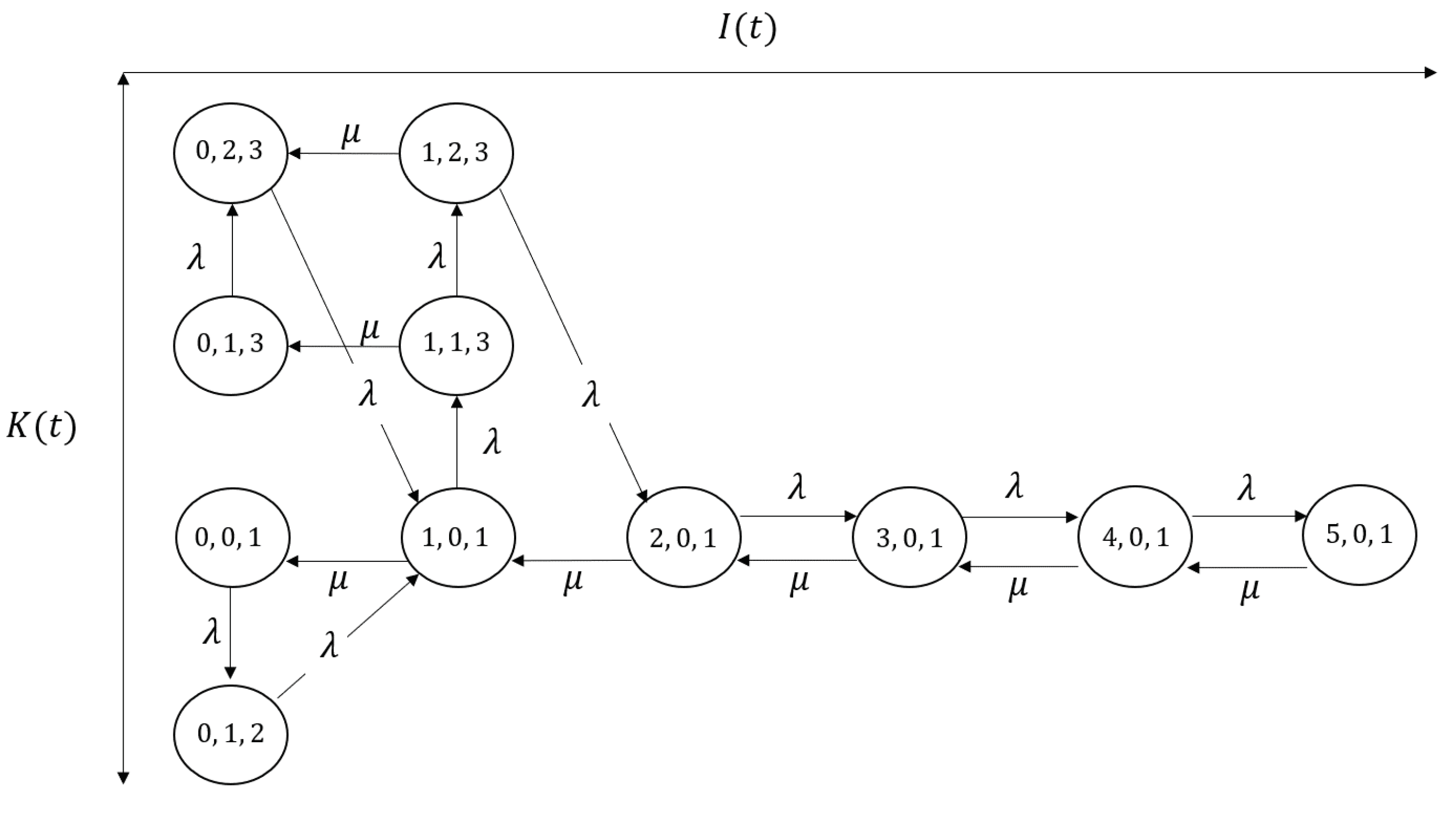
Figure 4 shows the transition diagram in which $l^{*}\left(0\right)=2,l^{*}\left(1\right)=3,l^{*}\left(2\right)=1$, $l^{*}\left(3\right)=1,l^{*}\left(4\right)=1,$ and $l^{*}\left(5\right)=0$ (thus, $i_{\left(\max \right)}=4,i_{(1*\min )}=2,i_{(2*\min )}=0,i_{(3*\min )}=1$, $i_{(1*\max )}=4,i_{(2*\max )}=0,i_{(3*\max )}=1,{\mathbb{B}}_{\left(0\right)}=\{1,2,3\},{\mathbb{B}}_{\left(1\right)}=\{1,3\},{\mathbb{B}}_{\left(2\right)}=\left\{1\right\}$, ${\mathbb{B}}_{\left(3\right)}=\left\{1\right\},{\mathbb{B}}_{\left(4\right)}=\left\{1\right\}$).

It should be mentioned that our algorithm in Theorem 1 enables us to consider the necessary and sufficient size of the transition diagram. We can also consider the Markov chain only by deriving $i_{\left(\max \right)}$ and the maximum best batch size as well; however, by utilizing Theorem 2, we can remove the unnecessary states (i.e., all the states $(i,k,l)$ such that $l\notin {\mathbb{B}}_{\left(i\right)},k\ge 1$ are removed in $\tilde{\mathcal{U}}$), for example, $(4,1,2)$ in Figure 3 and $(1,1,2),(2,1,2),(3,1,2),(2,1,3),(2,2,3),(3,1,3),$$(3,2,3),(4,1,3)$ and $(4,2,3)$ in Figure 4. The number of states decreases from 21 to 20 in Figure 3 and from 21 to 11 in Figure 4. It is expected that the state space in our Markov chain becomes extreme large as $i_{\left(\max \right)}$ becomes larger. Therefore, the calculation of ${\mathbb{B}}_{\left(i\right)}$ in Algorithm 1 is crucial from the perspective of the calculation cost (especially for preventing memory error). In addition, the rigorous proof in Lemma 5 also improves computational tractability. We can construct $\tilde{\mathcal{U}}$ and consider the corresponding transition rates between the states only by ${\mathbb{B}}_{\left(i\right)},i_{\left(\max \right)},i_{(l*\min )}$, and $i_{(l*\max )}$; therefore, we do not consider whether the transition $(i,0,1)\to (i,1,l)$ occurs for every i after deriving all $i_{(l*\min )}\mathrm{and}{i}_{(l*\max )}$. When $i_{\left(\max \right)}$ is large and the differences between $i_{(l*\min )}\mathrm{and}{i}_{(l*\max )}$ become larger, Lemma 5 is effective to construct $\tilde{\mathcal{U}}$ easily.

The Markov chain has a finite state space. Therefore, we can easily obtain the numerical values of the steady state probabilities:

$${\pi }_{i,k,l}:=\underset{t\to \infty }{lim}\mathrm{P}(I\left(t\right)=i,K\left(t\right)=k,L\left(t\right)=l),$$

(13)

which are utilized to calculate the performance measures. First, we present Theorem 3.

Theorem 3.

Let $B_{\mathrm{new}}$ denote the random variables for the batch size of a newly generated batch. Then, $\mathrm{E}\left[B_{\mathit{new}}\right]$ and its probability function $f_{\mathit{new}}\left(n\right)$ are expressed by

$$\mathrm{E}\left[B_{\mathit{new}}\right]={\displaystyle \frac{{\sum }_{i=0}^{i_{\left(\mathit{max}\right)}}{\sum }_{l\in {\mathbb{B}}_{\left(i\right)}}l{\pi }_{i,l-1,l}}{{\sum }_{i=0}^{i_{\left(\mathit{max}\right)}}{\sum }_{l\in {\mathbb{B}}_{\left(i\right)}}{\pi }_{i,l-1,l}}},$$

$$f_{\mathit{new}}\left(n\right)={\displaystyle \frac{{\sum }_{i=0}^{i_{\left(\mathit{max}\right)}}{\mathbb{1}}_{{\mathbb{B}}_{\left(i\right)}}\left[n\right]{\pi }_{i,n-1,n}}{{\sum }_{i=0}^{i_{\left(\mathit{max}\right)}}{\sum }_{l\in {\mathbb{B}}_{\left(i\right)}}{\pi }_{i,l-1,l}}},$$

where

$${\mathbb{1}}_A\left[x\right]=\left\{\begin{array}{c}1,(x\in A),\\ 0,(x\notin A),\end{array}\right.$$

(14)

respectively.

Proof. 

A new batch is generated when a customer joins the state $(K,L)=(l,l-1)$ according to the Poisson process at rate $\lambda$. Therefore, the total number of newly generated batches per unit time can be calculated as ${\sum }_{i=0}^{i_{\left(max\right)}}{\sum }_{l\in {\mathbb{B}}_{\left(i\right)}}\lambda {\pi }_{i,l-1,l}$, which is equivalent to the total rate of the transition from state $(K,L)=(l,l-1)$ to $K=0$. Additionally, the total number of customers served per unit time is calculated by ${\sum }_{i=0}^{i_{\left(max\right)}}{\sum }_{l\in {\mathbb{B}}_{\left(i\right)}}l\lambda {\pi }_{i,l-1,l}$. The latter divided by the former can clearly be the expected batch size. Similarly, the probability function is derived. □

In addition, we present the following theorem:

Theorem 4.

Let V denote a random variable for the number of newly generated batches per unit time. Then, $\mathrm{E}\left[V\right]$ is given by

$$\mathrm{E}\left[V\right]=\sum _{i=0}^{i_{\left(\mathit{max}\right)}}\sum _{l\in {\mathbb{B}}_{\left(i\right)}}\lambda {\pi }_{i,l-1,l}.$$

Proof. 

The total throughput for the transition in the number of waiting customers $l-1\to 0$ is equivalent to $\mathrm{E}\left[V\right]$. □

Notably, $\mathrm{E}\left[V\right]$ reflects traffic congestion on the road. Subsequently, we present Theorem 5.

Theorem 5.

The expected number of customers in the system $\mathrm{E}\left[N\right]$ is given as follows:

$$\mathrm{E}\left[N\right]=\lambda \left(\sum _{i=0}^{i_{\left(\mathit{max}\right)}}{\pi }_{i,0,1}{W}_{i,0,l^{*}\left(i\right)}+\sum _{i=0}^{i_{\left(\mathit{max}\right)}}\sum _{l\in {\mathbb{B}}_{\left(i\right)}}\sum _{k=1}^{l-1}{\pi }_{i,k,l}{W}_{i,k,l}\right).$$

(15)

Proof. 

The batch size of each position is not i.i.d. distributed (because the best batch sizes are state-dependent values on i); therefore, calculating the expected number of customers is difficult in the system directly. However, the Poisson arrivals see time averages (PASTA) property holds because customers arrive at the system according to a Poisson process. We can then calculate the expected sojourn time of customers $\mathrm{E}\left[W\right]$ by conditioning $W_{i,k,l}$, using the steady state probabilities of joining customers as follows:

$$\mathrm{E}\left[W\right]={\displaystyle \frac{1}{\left(1-{\pi }_{i_{\left(\max \right)}+1,0,1}\right)}}\left(\sum _{i=0}^{i_{\left(\max \right)}}{\pi }_{i,0,1}{W}_{i,0,l^{*}\left(i\right)}+\sum _{i=0}^{i_{\left(\max \right)}}\sum _{l\in {\mathbb{B}}_{\left(i\right)}}\sum _{k=1}^{l-1}{\pi }_{i,k,l}{W}_{i,k,l}\right).$$

(16)

By applying Little’s law, the results are clear. □

Based on the aforementioned discussion, we consider several performance measures in Theorem 6.

Theorem 6.

The throughput (TH), social welfare (SW), and monopolist’s revenue (MR) are given by

$$\begin{array}{c}\hfill TH=\lambda (1-{\pi }_{i_{\left(\mathit{max}\right)}+1,0,1})=\lambda \sum _{i=0}^{i_{\left(\mathit{max}\right)}}{\pi }_{i,0,1}+\lambda \sum _{i=0}^{i_{\left(\mathit{max}\right)}}\sum _{l\in {\mathbb{B}}_{\left(i\right)}}\sum _{k=1}^{l-1}{\pi }_{i,k,l},\end{array}$$

(17)

$$\begin{array}{c}\hfill SW=\lambda \sum _{i=0}^{i_{\left(\mathit{max}\right)}}\sum _{l\in {\mathbb{B}}_{\left(i\right)}}\sum _{k=1}^{l-1}{\pi }_{i,k,l}R+\lambda \sum _{i=0}^{i_{\left(\mathit{max}\right)}}{\pi }_{i,0,1}R-C\mathrm{E}\left[N\right],\end{array}$$

(18)

$$\begin{array}{c}\hfill MR=\lambda \sum _{i=0}^{i_{\left(\mathbf{max}\right)}}{\pi }_{i,0,1}{p}_{l^{*}\left(i\right)}+\lambda \sum _{i=0}^{i_{\left(\mathit{max}\right)}}\sum _{l\in {\mathbb{B}}_{\left(i\right)}}\sum _{k=1}^{l-1}{\pi }_{i,k,l}{p}_l.\end{array}$$

(19)

Here, $TH$, $SW$, and $MR$ are the expected number of customers served per unit time, the difference between the generated reward and time cost per unit time, and the sum of fees that the monopolist (administrator) can obtain per unit time, respectively.

The flow of the analysis in this section can be summarized as follows. First, the equilibrium strategy of the proposed model is given by Lemma 1. Specifically, the equilibrium strategy can be calculated by using the results of Lemmas 2 and 4. Lemma 3, i.e., the properties of $W_{i,k,l}$, is used to prove Lemmas 4 and 5. Lemma 5 provides an important property of the best batch size (and it will be mentioned in Remark 6 with intuitive interpretations in the numerical experiment section). Then, Theorem 2 gives the reconstructed Markov chain, which has the necessary and sufficient number of the states, for the proposed model provided that every customer adopts the equilibrium strategy by using the outputs of Algorithm 1 in Theorem 1. Finally, some performance measures for the reconstructed Markov chain are derived in Theorems 3–6.

4. Numerical Experiments

This section presents numerical results on the performance measures in the previous section and discusses the behavior of the proposed model. Here, we introduce the notions of ‘fixed fee’ and ‘sharing fee’. A fixed fee refers to the fee that all customers pay to receive the service, regardless of their batch size. The sharing fee refers to the fee for a batch, that is, the fee for a person is the sharing fee divided by the batch size. Let f and s denote fixed and sharing fees, respectively. In addition, the maximum batch size (corresponding to the capacity of cars in ride-sharing and shared taxis) is assumed to be m. Then, if customers belong to a batch of size l, they must pay $p_l=f+s/l$ ($1\le l\le m$). Considering these settings, the reward for a batch service of size l is given by

$$R_l=\left\{\begin{array}{cc}R-(f+s/l),\hfill & (1\le l\le m),\hfill \\ 0,\hfill & \left(otherwise\right).\hfill \end{array}\right.$$

In this section, the detailed parameter settings are presented in the captions of each graph. We compared the proposed model (referred to as the variable batch service model in the following section to clarify the distinction) with the regular (i.e., fixed) batch size model [26] of size K. If $K=1$, this becomes equivalent to Naor’s model [23]. As mentioned in Section 3, the variable batch service model encompasses Naor’s and the regular batch service models.

Notably, if no customers join the system according to the parameter settings, we assume that $TH$, $SW$, and $MR$ become 0. First, we note the following remark from Lemma 6:

Remark 1.

$l^{*}\left(i\right)$ becomes a non-decreasing function (except for the case of $l^{*}\left(i\right)=0$; that is, the customer balks in the setting of fees, that is, $p_l=f+s/l$.

Table 1. Best batch sizes conditional on i under $\lambda =5,\mu =2,R=3,s=1,s\in \left\{0.1,1,2\right\}$, $f\in \left\{0.1,0.5\right\},m=5\mathrm{and}C=1$.

$(\mathit{s},\mathit{f})$	$\mathit{i}=0$	$\mathit{i}=1$	$\mathit{i}=2$	$\mathit{i}=3$	$\mathit{i}=4$
$(0.1,0.1)$	1	1	2	3	0
$(0.1,0.5)$	1	1	2	3	0
$(1.0,0.1)$	2	3	4	5	0
$(1.0,0.5)$	2	3	4	5	0
$(2.0,0.1)$	3	4	5	5	0
$(2.0,0.5)$	3	4	5	5	0

summarizes the numerical results for the best batch size conditional on i, that is, the number of complete batches in the system when a tagged first-arriving customer arrives. Notably, 0 indicates that the best option for the customer is to balk. Clearly, the best batch size increases as i increases, as mentioned in Remark 1. This result leads us to presume that to prevent more serious traffic congestion, it is individually optimal for customers to tend to create large batches while sharing fees with other customers if the system is crowded.

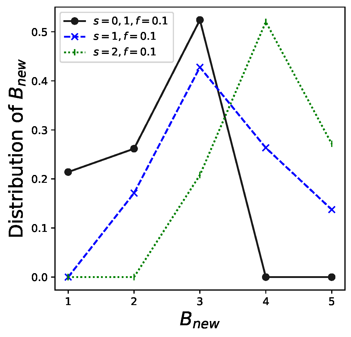
In addition, the distribution of $B_{\mathrm{new}}$, that is $f_{\mathrm{new}}\left(n\right)$, which is given by Theorem 3, is shown in Figure 5. We depict examples of $s\in \left\{0.1,1,2\right\}$ and $f=0.1$. The other parameter settings are the same as those in the example in Table 1. These results can be utilized for real-world management of this system. For example, the probabilities that $B_{\mathrm{new}}=4,5$ are 0 when $s=0.1$ and $f=0.1$. Therefore, three is sufficient for the capacity of cars, although the current setting for the maximum capacity of cars is $m=5$. This finding enables the system administrator to reduce excessive costs.

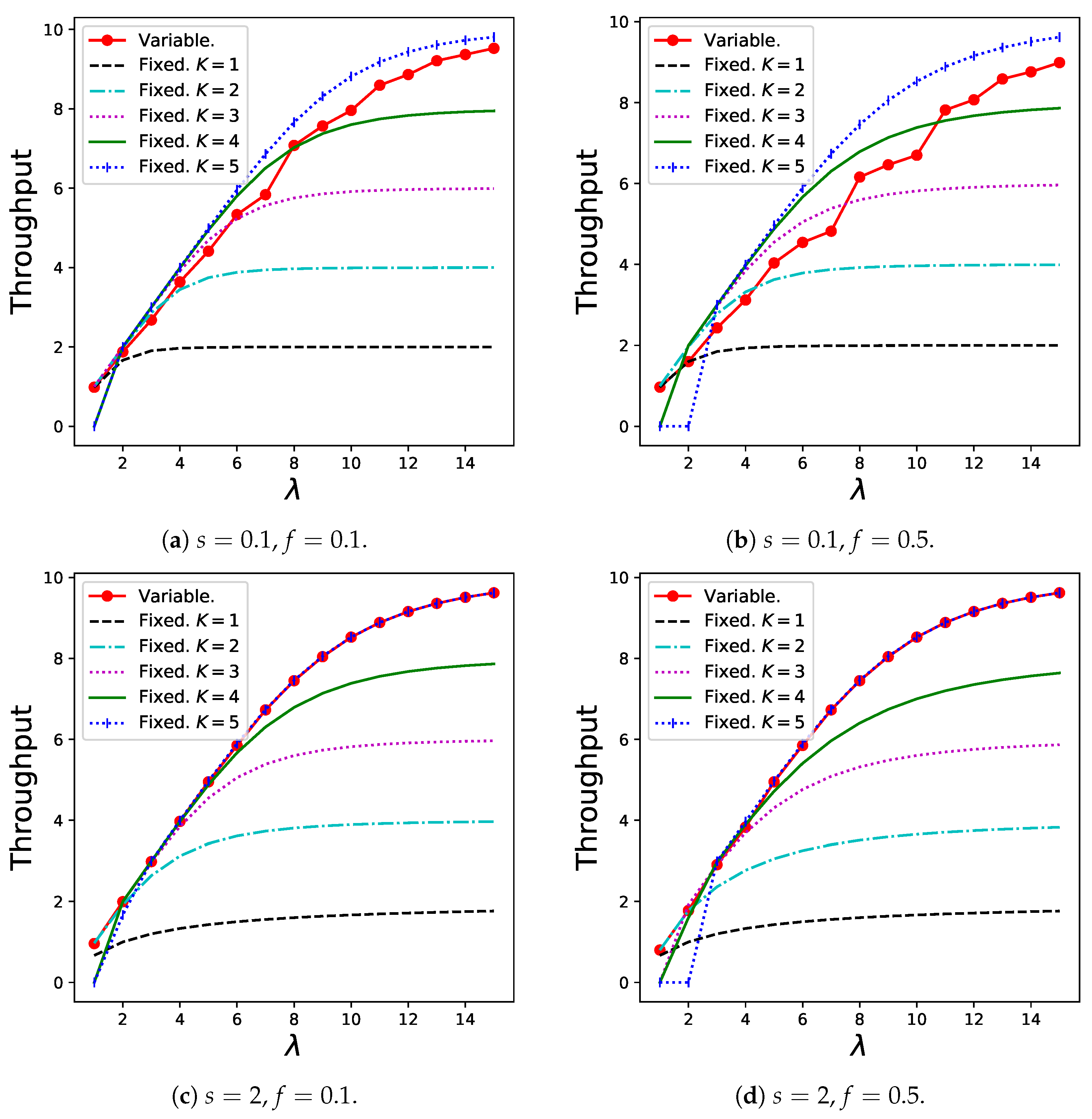
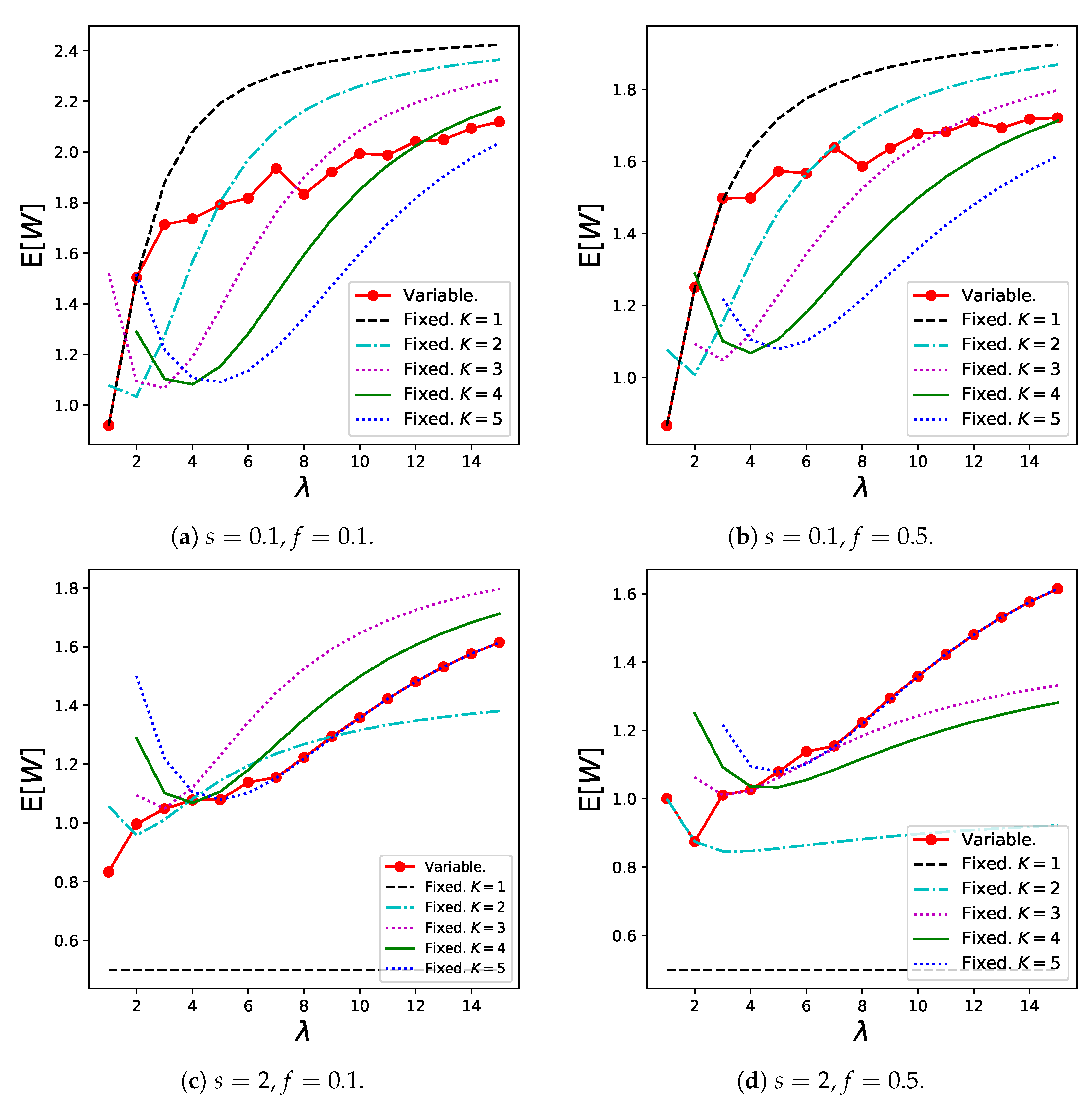
The results for the throughput $TH$ in Theorem 6 are shown in Figure 6. Generally, the variable batch service model shows the best results for any arrival rate $\lambda$ unless s is not extremely small because customers can choose the ideal batch sizes depending on $\lambda$, which prevents excessively long waiting times or traffic congestion that results in customers joining the system. Thus, the variable model is more robust to changing customer demands than the regular batch service model.

The reason for the poor performance of the variable batch service model when s is relatively low (Figure 6a,b) can be explained as follows: Customers tend to create small batches because the sharing fee that can be saved by creating a larger batch is less compared to the long expected waiting time in this case. This trend is presented in Table 1. However, if a considerably large number of small batches are generated, the congestion in the queue becomes serious, resulting in the balking of many customers. Therefore, a relatively large K (for example, $K=5$) is more desirable in these graphs from the throughput viewpoint.

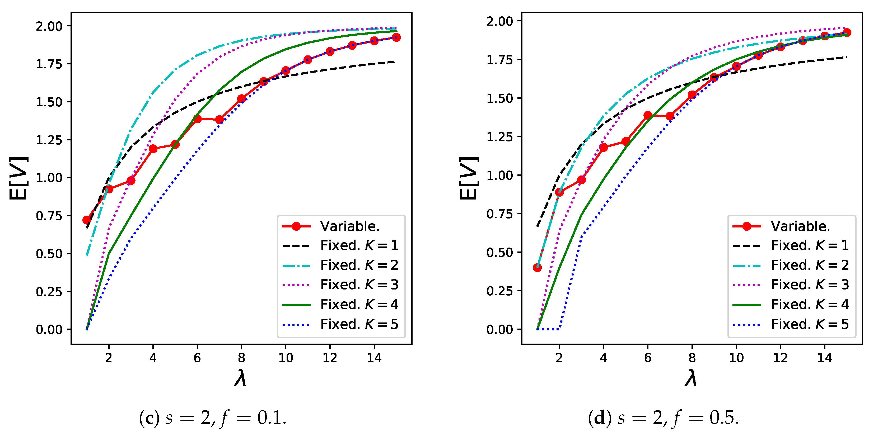
Figure 7 shows the results for social welfare, $SW$, in Theorem 6. The variable batch service model exhibited the best performance when s as well as $TH$ are relatively high. When $s=2$, the variable batch service model shows stable performance for any $\lambda$, whereas the regular batch service model with small batch sizes always shows poor performance, and the regular batch service model with large batch sizes shows poor results within the low $\lambda$ zone. Therefore, the variable batch service model can be considered robust against demand fluctuations when s is large.

However, we note that the variable batch service model shows very poor performance when s is low, because batches are generated excessively and induce congestion in the system. In other words, a system where customers behave individually does not necessarily lead to a socially optimal state. Therefore, as a practical message, it is important for an administrator to set s to a relatively high value to avoid this situation.

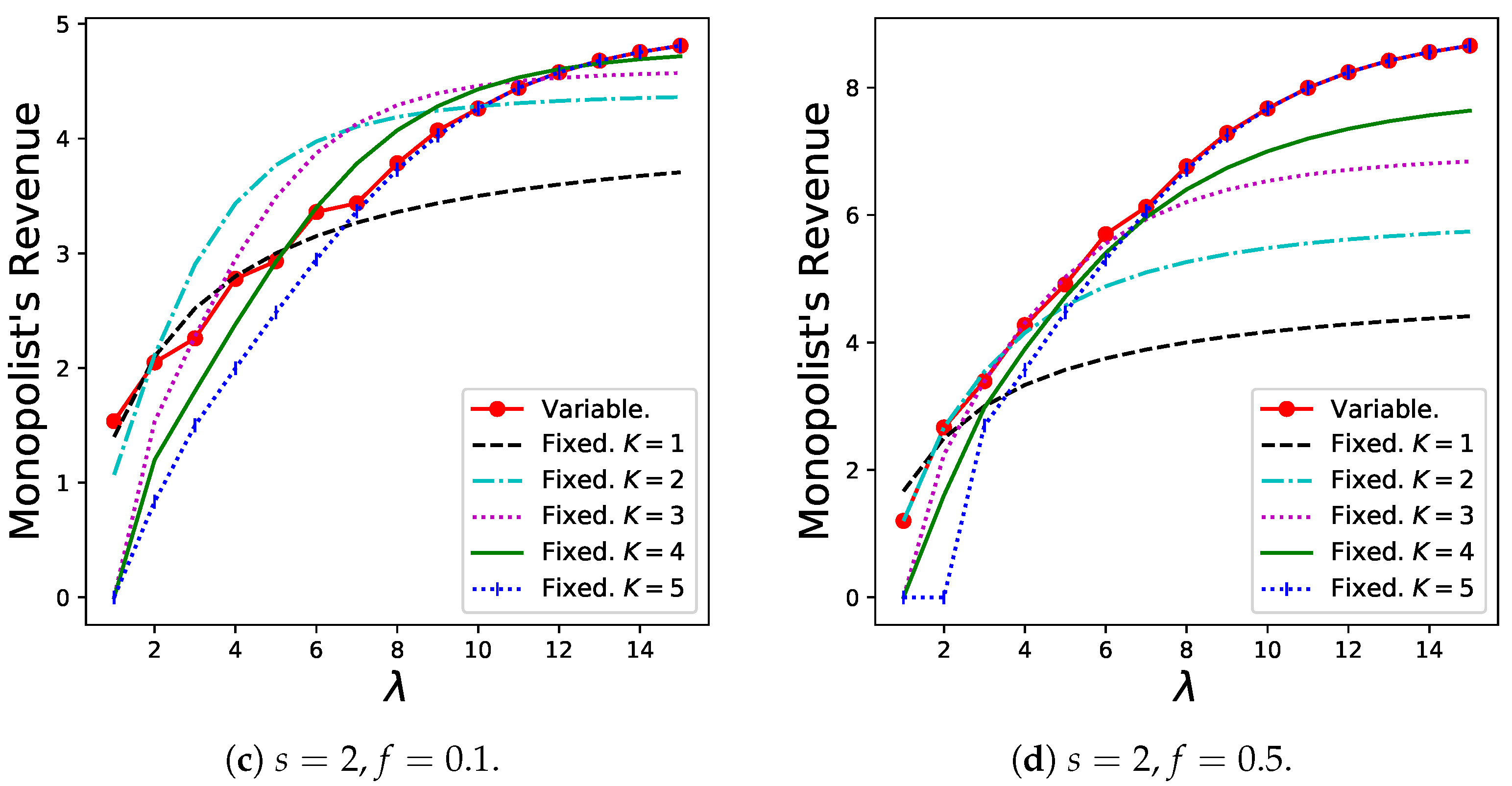
The results for the monopolist’s revenue, $MR$, are shown in Figure 8. The variable batch service model exhibits good performance as long as both s and f are relatively high (as in Figure 8d). However, especially when f is extremely small, the revenue of the variable batch service model decreases slightly.

The reasons for these results are as follows: In the variable batch-service model (compared with the regular batch service model), the following two effects were observed:

(i)

The increase in the throughput.

(ii)

The decrease in the number of batches in the system.

Effect (i) is presented in Table 1. Effect (ii) occurs because customers create larger batches if many batches already exist in the system to prevent serious congestion in the queue. When the fixed fee is low, the dominance of the total revenue is based only on the number of batches in the system that corresponds to the sharing fee. Specifically, the numerical results for the number of newly generated batches per unit time $\mathrm{E}\left[V\right]$ for the same parameters are shown in Figure 9. Therefore, in this case, effect (ii) increases, and revenue decreases. When a fixed fee is imposed to some extent, effect (i) increases as the arrival rate increases, and the total amount of fixed fees, which is proportional to the throughput, increases. Therefore, the administrator must set f as well as s to some high value.

Furthermore, it is worth noting that the variable batch service model is more suitable to optimize all of $TH$, $SW$, $MR$, simultaneously, compared to the regular batch service model, when the fees are properly set high ($s=2$ and $f=0.5$ in this example). See Figure 6d, Figure 7d, and Figure 8d. For $TH$ and $SW$, the variable batch service model and the regular batch service model with $K=5$ show the best performances when $\lambda \ge 3$. For $MR$, the variable batch service model and the regular batch service model with $K=5$ also show the best performances when $\lambda \ge 7$. On the other hand, when $4\le \lambda \le 6$, the variable batch service model and the regular batch service model with $K=3$ take better values in $MR$ than that of the regular batch service model with $K=5$. These results for the regular batch service model imply that the monopolist should set the batch size K smaller to maximize $MR$ compared to the batch size which maximizes $TH$ and $SW$. However, as has been shown, the variable batch service model enables all $TH$, $SW$, and $MR$ to be the best values simultaneously as long as the fees are set high properly.

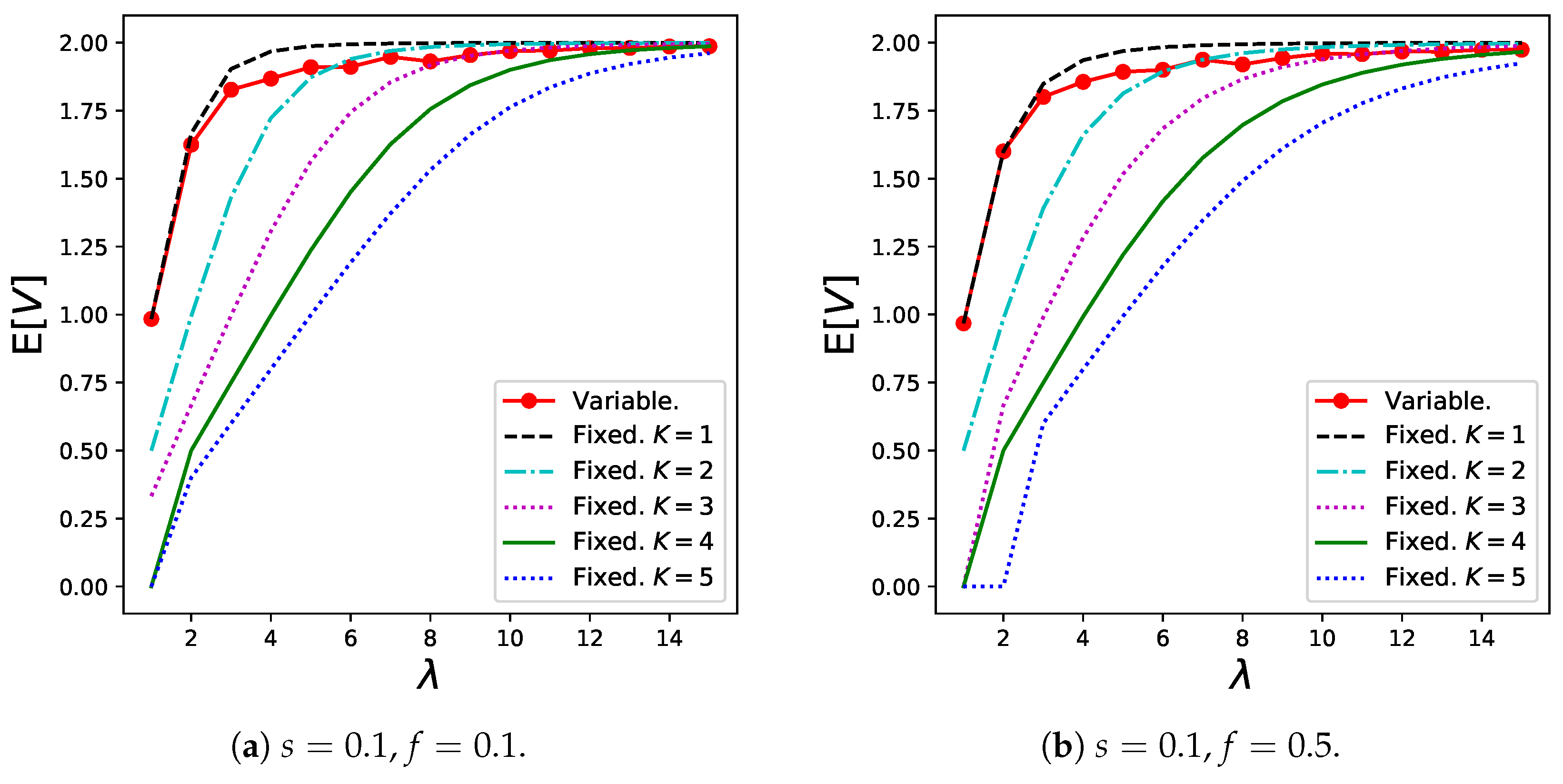
In addition, Figure 10 shows the numerical results for $\mathrm{E}\left[W\right]$, which are given by (16). The results for the variable batch service model generally increase as $\lambda$ increases, whereas most results for the regular batch service model have minimum points. This is because customers can reduce their batch sizes to prevent extremely long waiting times when the arrival rate is low.

Notably, $\mathrm{E}\left[W\right]$ in the variable batch service model is lower than that in the regular batch service model in which $TH$ and $SW$ are close to those in the variable batch service model under the specific parameter setting, for example, when $\lambda =3$ in Figure 6d, Figure 7d, and Figure 10d, respectively. Therefore, from the waiting time perspective, a variable batch service model is preferred in this case as well. On the contrary, the regular batch service model with $K=1$ shows the best performance when $\lambda =1$ from the perspective of $\mathrm{E}\left[W\right]$ and the other three performance measures.

We note that the tendency of the results of $\mathrm{E}\left[W\right]$ does not necessarily coincide with that of $SW$ in Figure 7. This is because $\mathrm{E}\left[W\right]$ does not reflect information of balking customers. For example, the results for $K=1,2$ within high $\lambda$ zone in Figure 7d show extremely small values because the dominant customers abandon the service (as can be confirmed in Figure 6d). Therefore, a small $\mathrm{E}\left[W\right]$ does not always imply superiority from a system point of view. However, the results for $\mathrm{E}\left[W\right]$ are valuable from a customer’s perspective. The proposed model is useful in obtaining numerous performance measures from various perspectives.

5. Conclusions

In this study, we proposed a variable batch service model in which first-arriving customers can select the batch size flexibly to maximize their individual utility. We formulated this model as a three-dimensional Markov chain and created a book-type transition diagram. We then demonstrated several properties of the sojourn time of a tagged customer and the best batch sizes, conditional on the number of complete batches in the system. Based on these properties, we proposed an effective algorithm to construct a necessary and sufficient size of state space for the Markov chain provided that all customers adopt the threshold-type equilibrium strategy.

Furthermore, we proved that the best batch size, provided that a tagged customer observes i complete batches in the system upon arrival, is a non-decreasing function for i if the reward for the completion of a batch service with size l is an increasing function of l; in other words, the fee decreases as the batch becomes larger. This implies that to prevent more serious traffic congestion, creating large batches while sharing fees with other customers is individually optimal for customers if the system is crowded.

In the numerical experiment, we showed several results on performance measures, throughput, social welfare, monopolist’s revenue, and expected sojourn time, and compared them with the regular batch service model [26]. The proposed model showed better performance when the fixed and sharing fees were relatively high. In addition, the proposed model does not show extremely poor results for any arrival rate as long as both fees are set in a well-balanced manner compared to the regular batch size model. This indicates that the present model is a robust model for the fluctuation of customer demand. Moreover, we showed that the introduction of the variable batch service model can lead to optimizing all of the throughput, social welfare, and monopolist’s revenue, simultaneously, compared to the regular batch service model when the fees were relatively high.

However, the proposed model performed poorly when fees were low. Therefore, a system in which customers select optimal batch sizes individually does not necessarily lead to a socially optimal state. Thus, it is important to set both fixed and sharing fees to some extent for the administrator in this system.

Further studies of the variable batch service model must consider the mechanism by which all customers (including non-first-arriving customers) can freely select their batch sizes. Analysis of this model is difficult; however, the change in performance is intriguing.